Mc-Donald modified Burr-III distribution: properties and applications

ABSTRACT

We propose herein a six-parameter McDonald modified Burr-III distribution. This distribution contains several special cases, including the modified Burr-III, Burr-III, Beta Burr-III, and Kum Burr-III distributions. Accordingly, we obtained its hazard function, survival function, moments, Renyi’s entropy, β-entropy, and mean deviation. We also used the method of maximum likelihood to estimate the parameters of our proposed distribution. Simulation studies were also performed for different values of sample sizes. The proposed model is applied on real-life datasets and shows that our proposed distribution yields better fits than other existing models.

KEYWORDS:

• Mc-Donald modified Burr-III
• Burr-III distribution
• parameters
• deviation
• real life data sets
• Renyi’s entropy
• Beta entropies

MATHEMATICS SUBJECT CLASSIFICATIONS:

• Primary 62F15
• Secondary 65

1. Introduction

1.1. Burr–III distribution

Burr [1] introduced a system based on twelve types of cumulative distribution functions. These cumulative distribution functions are based on the Pearson system of distributions which have a variety of density shapes. The Burr system is valid for a large range of applications. Based on the system of Burr distributions, the Burr–XII distribution is a commonly used model. The Burr–III distribution has also been used in various settings for statistical modelling. Gove et al. [2] and Lindsay et al. [3] used the Burr–III distribution in forestry. The Burr–III model was used by Nadarajah [4] and Kotz [5] in fracture roughness, and by Wingo [6,7] in life testing. Additionally, the model was also used by Chernobai et al. [8] for operational risks and by Sherrick et al. [9] for option market price distributions. In turn, Mielke and Paul [10] used it in meteorology, Tejeda and Goodwin used it to model rice crops [11], and Abdel-Ghaly et al. [12] used it in reliability analyses.

The Burr–III distribution is the inverse of the BX–II distribution. The Burr–III distribution is used in various fields of science. In studies of wages, wealth, and income, the Burr–III distribution is called the Degum distribution [13]. The Burr–III distribution is either equal to the inverse of the Burr distribution [14] or the inverse of the kappa distribution [10] in the respective literatures of actuarial and meteorological sciences. The extended Burr–III distribution was also used in low-flow frequency analyses by Shao et al. [15].

Ali et al. [16] defined MB–III as (1) $F\left(x\right)=[1+\gamma x^{-\beta }{]}^{-\frac{\alpha }{\gamma }},\alpha ,\beta ,\gamma >0,x>0$(1) (2) $\begin{array}{rl}& \text{Accordingly, the pdf of the MB-III is}f\left(x\right)\\ & =\alpha \beta x^{-\beta -1}[1+\gamma x^{-\beta }{]}^{-\frac{\alpha }{\gamma }-1},\end{array}$(2) where $\alpha ,\beta$, and $\gamma$, are the shape parameters of the MB–III distribution. The limiting distribution for $\gamma \to 0$ of the modified Burr–III distribution becomes a generalized inverse Weibull distribution as indicated by Gusmao et al. [17]. If $\gamma =1$, the MB–III distribution becomes the Burr–III distribution [1]. The modified Burr–III distribution reduces to a log–logistic distribution if $\alpha =\gamma =1$ and if a scale parameter is added, as indicated by Shoukri et al. [18].

2. McDonald modified Burr–III (McMB–III) distribution

2.1. McMB–III distribution

If the random variable x follows an McMB–III distribution, then it is defined as (3) $\begin{array}{rl}F\left(x\right)& =\frac{1}{B(\lambda ,\eta )}\sum _{j=0}^{\mathrm{\infty }}\frac{{(-1)}^j\mathrm{\Gamma }\eta }{\mathrm{\Gamma }(\eta -j)j!}\frac{1}{\left(\lambda +j\right)}\\ & \times (1+\gamma x^{-\beta }{)}^{-\frac{\alpha \xi }{\gamma }\left(\lambda +j\right)},\alpha ,\beta ,\gamma ,\lambda ,\eta ,\xi >0,x>0\end{array}$(3) where the probability density function is (4) $\begin{array}{rl}& f(x;\alpha ,\beta ,\gamma ,\lambda ,\eta ,\xi )\\ & =\frac{\xi \alpha \beta }{B(\lambda ,\eta )}{x}^{-\beta -1}(1+\gamma x^{-\beta }{)}^{-\frac{\lambda \xi \alpha }{\gamma }-1}\\ & \times {\left(1-{\left(1+\gamma x^{-\beta }\right)}^{-\frac{\alpha \xi }{\gamma }}\right)}^{\eta -1}\end{array}$(4) where $\alpha ,\beta ,\gamma ,\lambda ,\eta ,\xi$ are the shape parameters.

The survival function of the McMB–III distribution is given by (5) $\begin{array}{rl}S\left(x\right)& =1-\left(\frac{1}{B(\lambda ,\eta )}\sum _{j=0}^{\mathrm{\infty }}\frac{{(-1)}^j\mathrm{\Gamma }\eta }{\mathrm{\Gamma }(\eta -j)j!}\frac{1}{\left(\lambda +j\right)}\right.\\ & \times \left.{\left(1+\gamma x^{-\beta }\right)}^{-\frac{\alpha \xi }{\gamma }\left(\lambda +j\right)}\phantom{\sum _{j=0}^{\mathrm{\infty }}}\right)\end{array}$(5)

The Hazard function of the McMB–III distribution can be defined as (6) $h\left(x\right)=\frac{\begin{array}{c}\frac{\xi \alpha \beta }{B(\lambda ,\eta )}{x}^{-\beta -1}{\left(1+\gamma x^{-\beta }\right)}^{(-\lambda \xi \alpha /\gamma )-1}\\ (1-{\left(1+\gamma x^{-\beta }\right)}^{(-\alpha \xi /\gamma )}{)}^{\eta -1}\end{array}}{1-\left(\frac{1}{B(\lambda ,\eta )}\sum _{j=0}^{\mathrm{\infty }}\frac{{(-1)}^j\mathrm{\Gamma }\eta }{\mathrm{\Gamma }(\eta -j)j!}\frac{1}{\left(\lambda +j\right)}{\left(1+\gamma x^{-\beta }\right)}^{-\frac{\alpha \xi }{\gamma }\left(\lambda +j\right)}\right)}$(6)

Plots of the pdf, CDF, survival function, and hazard function for various values of $\alpha ,\beta ,\gamma ,\lambda ,\eta ,\xi$, are given below Figures 1 and 2.

Figure 1. PDF plot of the McMB–III distribution.

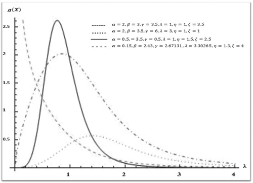
Figure 2 Hazard plot of the McMB–III distribution.

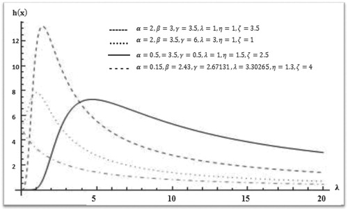
The graphs of (3) for various values of $\alpha ,\beta ,\gamma ,\lambda ,\eta ,\xi$ are plotted in Figure 3 and Table 1.

Figure 3. (a) Effect of α for fixed $\beta ,\gamma ,\lambda ,\eta$, and $\xi$values. (b) Effect of $\beta$ for fixed $\alpha ,\gamma ,\lambda ,\eta$, and $\xi$ values. (c) Effect of $\gamma$ for fixed $\alpha ,\beta ,\lambda ,\eta$, and $\xi$ values. (d) Effect of $\lambda$ for fixed $\alpha ,\beta ,\gamma ,\eta$, and $\xi$ values. (e) Effect of $\eta$ for fixed $\alpha ,\beta ,\gamma ,\lambda ,$ and $\xi$ values. (f) Effect of $\xi$ for fixed $\alpha ,\beta ,\gamma ,\lambda$, and $\eta$ values.

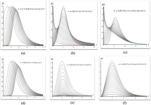
Table 1. Summary of some special cases of the McMB–III distribution.

	Parameters
Distribution	$\alpha$	$\beta$	$\gamma$	$\lambda$	$\eta$	$\xi$	Distribution Name
MB–III	$\alpha$	$\beta$	$\gamma$	1	1	1	Modified Burr–III distribution
B–III	$\alpha$	$\beta$	1	1	1	1	Burr–III distribution
McB–III	$\alpha$	$\beta$	1	$\lambda$	$\eta$	$\xi$	McDonald Burr–III distribution
BMB–III	$\alpha$	$\beta$	$\gamma$	$\lambda$	$\eta$	1	Beta modified Burr–III distribution
BBIII	$\alpha$	$\beta$	1	$\lambda$	$\eta$	1	Beta Burr–III distribution
KMBIII	$\alpha$	$\beta$	$\gamma$	1	$\eta$	$\xi$	Kumarasamy modified Burr–III distribution
KBIII	$\alpha$	$\beta$	1	1	$\eta$	$\xi$	Kumarasamy Burr–III distribution
EMBIII	$\alpha$	$\beta$	$\gamma$	1	1	$\xi$	Exponential modified Burr–III distribution
EBIII	$\alpha$	$\beta$	1	1	1	$\xi$	Exponential Burr–III distribution
MLL	1	$\beta$	1	$\lambda$	$\eta$	$\xi$	Modified Log–Logistic distribution
KLL	1	$\beta$	1	1	$\eta$	$\xi$	Kumarasamy Log–Logistic distribution
BLL	1	$\beta$	1	$\lambda$	$\eta$	1	Beta Log–Logistic distribution
LL	1	$\beta$	1	1	1	1	Log–Logistic distribution

3. Properties of McMB–III distribution

In this section, we derive some basic properties and useful features for McMB–III, including the survival function, hazard rate function, moments, mean deviation, entropies, etc.

3.1. Moments of McMB–III distribution

In this subsection we discuss the k^th moments for the McMB–III distribution. Moments are necessary and important in any statistical analyses, especially in different types of applications. It can be used to study the most important features and characteristics of a distribution (e.g. tendency, dispersion, skewness, and kurtosis).

The k^th moments of the McMB–III distribution are obtained as (7) ${\mu }_{{}_k}^{\mathrm{\prime }}=\frac{\xi \alpha {\gamma }^{k/\beta }}{\gamma B(\lambda ,\eta )}\sum _{j=1}^{\mathrm{\infty }}\frac{{(-1)}^j\mathrm{\Gamma }\eta }{\mathrm{\Gamma }(\eta -j)j!}B\left(A_k,B_k\right)$(7) where $B\left(A_k,B_k\right)$ is a beta function, $A_k=\frac{k}{\beta }+\frac{\alpha \xi }{\gamma }(\lambda +j),B_k=1-\frac{k}{\beta }$ and $k<\beta$, 1< k/β and k/β should not be integers.

The negative moments for the McMB–III distribution are expressed according to (8) $\begin{array}{rl}{\mu }_{-r}^{\mathrm{\prime }}& =\frac{\xi \alpha {\gamma }^{-r/\beta }}{\gamma B(\lambda ,\eta )}\sum _{j=1}^{\mathrm{\infty }}\frac{{(-1)}^j\mathrm{\Gamma }\eta }{\mathrm{\Gamma }(\eta -j)j!}B\\ & \times \left(\frac{\alpha \xi }{\gamma }(\lambda +j)-\frac{r}{\beta },1+\frac{r}{\beta }\right)\end{array}$(8) where $\frac{\alpha \xi }{\gamma }(\lambda +j)>\frac{r}{\beta },\frac{\alpha \xi }{\gamma }(\lambda +j)<\frac{r}{\beta },$ and $r/\beta$ should not be integers.

The factorial moments of the McMB–III distribution are expressed by (9) $\begin{array}{rl}{\mu }_{\left(r\right)}^{\mathrm{\prime }}& =E\left[x^{\left(r\right)}\right]=E\left(x\left(x-1\right)\left(x-2\right)\cdots \left(x-k+1\right)\right)\\ & =\sum _{k=0}^{n}S\left(n,k\right)E\left(x^k\right)\end{array}$(9)

Substitution of (7) in (9) leads to, (10) $\begin{array}{rl}{\mu }_{\left(r\right)}^{\mathrm{\prime }}& =\sum _{k=0}^{n}S\left(n,k\right)\frac{\xi \alpha {\gamma }^{k/\beta }}{\gamma B(\lambda ,\eta )}\sum _{j=1}^{\mathrm{\infty }}\frac{{(-1)}^j\mathrm{\Gamma }\eta }{\mathrm{\Gamma }(\eta -j)j!}B\\ & \times \left(\frac{k}{\beta }+\frac{\alpha \xi }{\gamma }(\lambda +j),1-\frac{k}{\beta }\right)\end{array}$(10) where $1-\frac{k}{\beta }>0,\beta >k1-\frac{k}{\beta }<0,\frac{k}{\beta }$ should not be integers. $S\left(n,k\right)=(k!{)}^{-1}{\left[\frac{d^k}{d{x}^k}{x}^{\left(r\right)}\right]}_{x=0}$ is the Stirling number of the first kind and estimates the number of ways to permute a list of r items into k cycles.

The fractional moments for the McMB–III distribution are defined as (11) $\begin{array}{rl}E\left(x^{\frac{1}{r}}\right)& =\frac{\xi \alpha {\gamma }^{-1/r\beta }}{\gamma B(\lambda ,\eta )}\sum _{j=1}^{\mathrm{\infty }}\frac{{(-1)}^j\mathrm{\Gamma }\eta }{\mathrm{\Gamma }(\eta -j)j!}B\\ & \times \left(\frac{\alpha \xi }{\gamma }(\lambda +j)-\frac{1}{r\beta },1+\frac{1}{r\beta }\right)\end{array}$(11) where $\frac{\alpha \xi }{\gamma }(\lambda +j)>\frac{1}{r\beta },\frac{\alpha \xi }{\gamma }(\lambda +j)<\frac{1}{r\beta },$ and $1/r\beta$ should not be integers.

The mean and variance of the McMB–III distribution are given as (12) $\begin{array}{rl}\mu & =E\left(x\right)=\frac{\xi \alpha {\gamma }^{1/\beta }}{\gamma B(\lambda ,\eta )}\sum _{j=1}^{\mathrm{\infty }}\frac{{(-1)}^j\mathrm{\Gamma }\eta }{\mathrm{\Gamma }(\eta -j)j!}B\\ & \times \left(\frac{1}{\beta }+\frac{\alpha \xi }{\gamma }(\lambda +j),1-\frac{1}{\beta }\right)\end{array}$(12) (13) $\begin{array}{rl}Var\left(x\right)& =\frac{\xi \alpha {\gamma }^{2/\beta }}{{\left(\gamma B(\lambda ,\eta )\right)}^2}\sum _{j=1}^{\mathrm{\infty }}\frac{{(-1)}^j\mathrm{\Gamma }\eta }{\mathrm{\Gamma }(\eta -j)j!}\\ & \times \left[B\left(\frac{2}{\beta }+\frac{\alpha \xi }{\gamma }(\lambda +j),1-\frac{2}{\beta }\right)\right.\\ & -\left.B^2\left(\frac{1}{\beta }+\frac{\alpha \xi }{\gamma }(\lambda +j),1-\frac{1}{\beta }\right)\right]\end{array}$(13)

The central moments are (14) $\begin{array}{rl}{\mu }_r& =\sum _{i=0}^r\left(\begin{array}{c}r\\ i\end{array}\right){\left(-1\right)}^i{\left(\frac{\xi \alpha }{\gamma B(\lambda ,\eta )}\right)}^{i+1}{\gamma }^{\frac{r-i}{\beta }+\frac{i}{\beta }}\\ & \times {\left(\sum _{j=1}^{\mathrm{\infty }}\frac{{(-1)}^j\mathrm{\Gamma }\eta }{\mathrm{\Gamma }(\eta -j)j!}B\left(A_1,B_1\right)\right)}^i\\ & \times \sum _{j=1}^{\mathrm{\infty }}\frac{{(-1)}^j\mathrm{\Gamma }\eta }{\mathrm{\Gamma }(\eta -j)j!}B\left(A_{r-i},B_{r-i}\right)\end{array}$(14)

Correspondingly, the cumulants are (15) $\begin{array}{rl}{\kappa }_r& =\frac{\xi \alpha }{\gamma B(\lambda ,\eta )}\left({\gamma }^{\frac{r}{\beta }}\sum _{j=1}^{\mathrm{\infty }}\frac{{(-1)}^j\mathrm{\Gamma }\eta }{\mathrm{\Gamma }(\eta -j)j!}B\left(A_r,B_r\right)-\sum _{i=1}^{r-1}\right.\\ & \times \left.\left(\begin{array}{c}r-1\\ i-1\end{array}\right){\kappa }_i{\gamma }^{\frac{\left(r-i\right)}{\beta }}\sum _{j=1}^{\mathrm{\infty }}\frac{{(-1)}^j\mathrm{\Gamma }\eta }{\mathrm{\Gamma }(\eta -j)j!}B\left(A_{r-i},B_{r-i}\right)\right)\end{array}$(15) where ${\kappa }_1={\mu }_1^{\mathrm{\prime }}$, then ${\kappa }_2={\mu }_2^{\mathrm{\prime }}-{\mu }_1^{\mathrm{\prime }2},{\kappa }_3={\mu }_3^{\mathrm{\prime }}-3{\mu }_2^{\mathrm{\prime }}{\mu }_1^{\mathrm{\prime }}+2{\mu }_1^{\mathrm{\prime }3},{\kappa }_4={\mu }_4^{\mathrm{\prime }}-4{\mu }_3^{\mathrm{\prime }}{\mu }_1^{\mathrm{\prime }}-3{\mu }_2^{\mathrm{\prime }2}+12{\mu }_2^{\mathrm{\prime }}{\mu }_1^{\mathrm{\prime }2}-6{\mu }_1^{\mathrm{\prime }4}$, etc.

Additionally, the coefficient of skewness is (16) $\sqrt{{\beta }_1}=\frac{\begin{array}{c}\sum _{i=0}^3\left(\begin{array}{c}3\\ i\end{array}\right){\left(-1\right)}^i{\left(\frac{\xi \alpha }{\gamma B(\lambda ,\eta )}\right)}^{i+1}{\gamma }^{\left(3-i\right)/\beta +\frac{i}{\beta }}\\ {\left(\sum _{j=1}^{\mathrm{\infty }}\frac{{(-1)}^j\mathrm{\Gamma }\eta }{\mathrm{\Gamma }(\eta -j)j!}B\left(A_1,B_1\right)\right)}^i\sum _{j=1}^{\mathrm{\infty }}\frac{{(-1)}^j\mathrm{\Gamma }\eta }{\mathrm{\Gamma }(\eta -j)j!}B\left(A_{3-i},B_{3-i}\right)\end{array}}{\begin{array}{c}\left[\phantom{\sum _{j=1}^{\mathrm{\infty }}}\sum _{i=0}^2\left(\begin{array}{c}2\\ i\end{array}\right){\left(-1\right)}^i{\left(\frac{\xi \alpha }{\gamma B(\lambda ,\eta )}\right)}^{i+1}{\gamma }^{\left(2-i\right)/\beta +\frac{i}{\beta }}\right.\\ {\left(\sum _{j=1}^{\mathrm{\infty }}\frac{{(-1)}^j\mathrm{\Gamma }\eta }{\mathrm{\Gamma }(\eta -j)j!}B\left(A_1,B_1\right)\right)}^i\\ {\left.\sum _{j=1}^{\mathrm{\infty }}\frac{{(-1)}^j\mathrm{\Gamma }\eta }{\mathrm{\Gamma }(\eta -j)j!}B\left(A_{2-i},B_{2-i}\right)\right]}^{3/2}\end{array}},$(16)

Equivalently, the coefficient of kurtosis is (17) $\sqrt{{\beta }_1}=\frac{\begin{array}{c}\sum _{i=0}^3\left(\begin{array}{c}3\\ i\end{array}\right){\left(-1\right)}^i{\left(\frac{\xi \alpha }{\gamma B(\lambda ,\eta )}\right)}^{i+1}{\gamma }^{\left(3-i\right)/\beta +\frac{i}{\beta }}\\ {\left(\sum _{j=1}^{\mathrm{\infty }}\frac{{(-1)}^j\mathrm{\Gamma }\eta }{\mathrm{\Gamma }(\eta -j)j!}B\left(A_1,B_1\right)\right)}^i\sum _{j=1}^{\mathrm{\infty }}\frac{{(-1)}^j\mathrm{\Gamma }\eta }{\mathrm{\Gamma }(\eta -j)j!}B\left(A_{3-i},B_{3-i}\right)\end{array}}{\begin{array}{c}\left[\phantom{\sum _{j=1}^{\mathrm{\infty }}}\sum _{i=0}^2\left(\begin{array}{c}2\\ i\end{array}\right){\left(-1\right)}^i{\left(\frac{\xi \alpha }{\gamma B(\lambda ,\eta )}\right)}^{i+1}{\gamma }^{\left(2-i\right)/\beta +\frac{i}{\beta }}\right.\\ {\left(\sum _{j=1}^{\mathrm{\infty }}\frac{{(-1)}^j\mathrm{\Gamma }\eta }{\mathrm{\Gamma }(\eta -j)j!}B\left(A_1,B_1\right)\right)}^i\\ {\left.\sum _{j=1}^{\mathrm{\infty }}\frac{{(-1)}^j\mathrm{\Gamma }\eta }{\mathrm{\Gamma }(\eta -j)j!}B\left(A_{2-i},B_{2-i}\right)\right]}^{3/2}\end{array}},$(17)

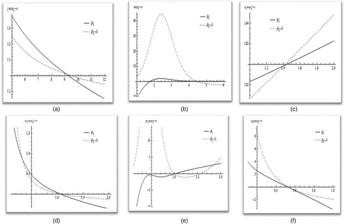
Furthermore, we plot ${\beta }_1$ and ${\beta }_2$-3 for the values of $\alpha ,\beta ,\gamma ,\lambda ,\eta \mathrm{\&}\xi .$

In Figure 4(a) both ${\beta }_1$ and ${\beta }_2$-3 approximately touch the x-axis. Thus, for $\beta =4.43,\gamma =1.5,\lambda =1.15,\eta =1,\xi =0.53$, the McMB–III distribution is approximately symmetrical. In Figure 4(b), we fix the values of $\alpha ,\gamma ,\lambda ,\eta ,\xi$, and vary $\beta .$ Both ${\beta }_1$ and ${\beta }_2$-3 have values which are close to the x-axis. Therefore, at $\alpha =10,\beta =4.5,\gamma =1.5,\lambda =1,\eta =1,\xi =0.53$, the McMB–III distribution is almost symmetrical. Similarly, in Figure 4(c), we fix $\alpha ,\beta ,\lambda ,\eta ,\xi$, and vary $\gamma .$ Both ${\beta }_1$ and ${\beta }_2$-3 have values which are close to the x-axis. Thus, at $\alpha =9.24,\beta =4.43,\gamma =1.42,\lambda =1.148,\eta =1,\xi =0.53$, the MMB–III distribution is approximately symmetrical. In Figure 4(d), we fix the values of $\alpha ,\beta ,\gamma ,\eta ,\xi$, and vary $\lambda .$ Both ${\beta }_1$ and ${\beta }_2$-3 have values which are close to the x-axis. Thus, at $\alpha =10,\gamma =1.5,\lambda =1,\lambda =1.1,\eta =1,\xi =0.53$, the McMB–III distribution is approximately symmetrical. Similarly, in Figure 4(e), we fix $\alpha ,\beta ,\gamma ,\lambda ,\xi$, and vary $\eta .$ Both ${\beta }_1$ and ${\beta }_2$-3 have values which are close to the x-axis. Thus, at $\alpha =10,\beta =4.43,\gamma =1.5,\lambda =1.15,\eta =1.0,\xi =0.53$, the McMB–III distribution is approximately symmetrical. Similarly, in Figure 4(f), we set the values of $\alpha ,\beta ,\gamma ,\lambda ,\eta$, at 10, 4.43, 1.5, 1.15, and 0.53, respectively, and vary $\xi .$ For $\xi =0.5$, both ${\beta }_1$ and ${\beta }_2$-3 have values which are close to the x-axis. Thus, at $\alpha =10,\beta =4.43,\gamma =1.5,\lambda =1.15,\eta =0.53,\xi =0.5$, the MMB–III distribution is approximately symmetrical.

Figure 4. (a) $(\beta =4.43,\gamma =1.5,\lambda =1.15,\eta =1,\xi =0.53)$. (b) $(\alpha =10,\gamma =1.5,\lambda =1,\eta =1,\xi =0.53)$. (c) $(\alpha =9.24,\beta =4.43,\lambda =1.148,\eta =1,\xi =0.53)$. (d) $(\alpha =10,\beta =4.43,\gamma =1.15,\eta =1,\xi =0.53)$. (e) $(\alpha =10,\beta =4.43,\gamma =1.5,\lambda =1.15,\xi =0.53)$. (f) $(\alpha =10,\beta =4.43,\gamma =1.5,\lambda =1.15,\eta =0.53)$.

3.2. Incomplete moments of the McMB–III distribution

Assume that f(x) is the probability density function of the McMB–III distribution of X defined on (0, ∞). The incomplete moments of the McMB–III distribution are given as (18) $\begin{array}{rl}{m}_r& =\frac{\xi \alpha {\gamma }^{r/\beta }}{\gamma B(\lambda ,\eta )}\sum _{j=1}^{\mathrm{\infty }}\frac{{(-1)}^j\mathrm{\Gamma }\eta }{\mathrm{\Gamma }(\eta -j)j!}\\ & \times \left(1-\frac{{\left(1-{\left(1+\gamma x^{-\beta }\right)}^{-1}\right)}^b}{B\left(a,b\right)}\sum _{i=0}^{a-1}{\left(-1\right)}^i\right.\\ & \times \left.\left(\begin{array}{c}a-1\\ i\end{array}\right)\frac{{\left(1-{\left(1+\gamma x^{-\beta }\right)}^{-1}\right)}^i}{b+i}\right)\end{array}$(18) where $a=\frac{r}{\beta }+\frac{\lambda \xi \alpha }{\gamma }+\frac{\alpha \xi j}{\gamma },b=1-\frac{r}{\beta },$ and $\frac{\alpha \xi }{\gamma }(\lambda +j)\ge \frac{r}{\beta },\beta \ge r$

3.3. Doubly truncated moments of McMB–III distribution

Assume that f(x) is the probability density function of the McMB–III distribution of X defined on (0, ∞). Doubly truncated moments of McMB–III are expressed according to (19) $\begin{array}{rl}& E\left(\frac{x^r}{t_1\le x\le t_2}\right)\\ & =\frac{{\gamma }^{r/\beta }}{\beta }\frac{\begin{array}{c}\sum _{j=0}^{\mathrm{\infty }}\frac{{(-1)}^j\mathrm{\Gamma }\eta }{\mathrm{\Gamma }(\eta -j)j!}\sum _{i=0}^{\mathrm{\infty }}\frac{\mathrm{\Gamma }\left(\frac{r}{\beta }\right)}{\mathrm{\Gamma }\left(\frac{r}{\beta }-i\right)i!}\\ \frac{\begin{array}{c}(1+\gamma t_2^{-\beta }{)}^{-\left(\right(r/\beta )+(\lambda \xi \alpha /\gamma )+(\alpha \xi j/\gamma )+i)}\\ -(1+\gamma t_1^{-\beta }{)}^{-\left(\right(r/\beta )+(\lambda \xi \alpha /\gamma )+(\alpha \xi j/\gamma )+i)}\end{array}}{\frac{r}{\beta }+\frac{\lambda \xi \alpha }{\gamma }+\frac{\alpha \xi j}{\gamma }+i}\end{array}}{\begin{array}{c}\sum _{j=0}^{\mathrm{\infty }}\frac{1}{\frac{\alpha \xi }{\gamma }\left(\lambda +j\right)+1}\frac{{(-1)}^j\mathrm{\Gamma }\eta }{\mathrm{\Gamma }(\eta -j)j!}\\ ({\left(1+\gamma {t_2}^{-\beta }\right)}^{(-\alpha \xi /\gamma )\left(\lambda +j\right)-1}\\ -{\left(1+\gamma {t_1}^{-\beta }\right)}^{(-\alpha \xi /\gamma )\left(\lambda +j\right)-1})\end{array}}\end{array}$(19)

3.4. Mean residual life (Moments of residual life)

The moments of mean residual life of the McMB–III are given as (20) $\begin{array}{rl}{M}_n\left(t\right)& =\frac{1}{1-F\left(t\right)}\frac{\xi \alpha \beta }{B(\lambda ,\eta )}\sum _{i=0}^n\frac{n!}{i!\left(n-i\right)!}{t}^{n-i}\\ & \times \sum _{j=0}^{\mathrm{\infty }}\frac{{(-1)}^j\mathrm{\Gamma }\eta }{\mathrm{\Gamma }(\eta -j)j!}{B}_{{\left(1+\gamma t^{-\beta }\right)}^{-1}}\\ & \times \left(\frac{i}{\beta }+\frac{\lambda \xi \alpha }{\gamma }+\frac{\xi \alpha }{\gamma }j,1-\frac{i}{\beta }\right)\end{array}$(20) where $1-\frac{i}{\beta }>0,\beta >i1-\frac{i}{\beta }<0,\frac{i}{\beta }$ should not be integers.

The reversed residual life moments can be obtained from (20) (21) $\begin{array}{rl}{M}_n\left(t\right)& ={\int }_t^{\mathrm{\infty }}{\left(x-t\right)}^{n}f\left(x\right)dx\\ M_n\left(t\right)& =\frac{\xi \alpha \beta }{B(\lambda ,\eta )}\sum _{i=0}^n\frac{n!}{i!\left(n-i\right)!}{t}^{n-i}\\ & \times \sum _{j=0}^{\mathrm{\infty }}\frac{{(-1)}^j\mathrm{\Gamma }\eta }{\mathrm{\Gamma }(\eta -j)j!}{B}_{{\left(1+\gamma t^{-\beta }\right)}^{-1}}\\ & \times \left(\frac{i}{\beta }+\frac{\lambda \xi \alpha }{\gamma }+\frac{\xi \alpha }{\gamma }j,1-\frac{i}{\beta }\right)\end{array}$(21)

3.5. Mean deviation of the McMMB–III distribution

The mean deviation about the mean and median can be used to measure the spread in a population. Accordingly, it can be expressed as ${\delta }_1\left(x\right)=E\left(-{\mu }_1^{\mathrm{\prime }}|\right)=2{\mu }_1^{\mathrm{\prime }}F\left({\mu }_1^{\mathrm{\prime }}\right)-2T_1\left({\mu }_1^{\mathrm{\prime }}\right)$ and ${\delta }_2\left(x\right)=E\left(-m|\right)={\mu }_1^{\mathrm{\prime }}-2T_1\left(m\right)$, where $T_1(.)$ is a doubly truncated moments in Eq. 19 and F (.) is distribution function in Eq. 3. The mean deviations about the mean and median are given below, $\begin{array}{rl}{\delta }_1\left(x\right)& =\frac{2{\mu }_1^{\mathrm{\prime }}\xi \alpha \beta }{\gamma B(\lambda ,\eta )}\frac{1}{\frac{\alpha \xi }{\gamma }\left(\lambda +j\right)+1}\\ & \times \sum _{j=0}^{\mathrm{\infty }}\frac{{(-1)}^j\mathrm{\Gamma }\eta }{\mathrm{\Gamma }(\eta -j)j!}{A_1}^{-\frac{\alpha \xi }{\gamma }\left(\lambda +j\right)-1}-\frac{2{\gamma }^{1/\beta }}{\beta }\\ & \times \frac{\sum _{j=0}^{\mathrm{\infty }}\frac{{(-1)}^j\mathrm{\Gamma }\eta }{\mathrm{\Gamma }(\eta -j)j!}{A}_2}{\sum _{j=0}^{\mathrm{\infty }}\frac{1}{\frac{\alpha \xi }{\gamma }\left(\lambda +j\right)+1}\frac{{(-1)}^j\mathrm{\Gamma }\eta }{\mathrm{\Gamma }(\eta -j)j!}{A_1}^{(-\alpha \xi /\gamma )\left(\lambda +j\right)-1}}\\ \text{Where }{A}_1& =1+\gamma \mu {{}_1^{\mathrm{\prime }}}^{-\beta },\\ A_2& =\sum _{i=0}^{\mathrm{\infty }}\frac{\mathrm{\Gamma }\left(\frac{1}{\beta }\right)}{\mathrm{\Gamma }\left(\frac{1}{\beta }-i\right)i!}\\ & \times \frac{A_1{{}^{-}}^{\left(\left(1/\beta \right)+\left(\lambda \xi \alpha /\gamma \right)+\left(\alpha \xi j/\gamma \right)+i\right)}}{\frac{1}{\beta }+\frac{\lambda \xi \alpha }{\gamma }+\frac{\alpha \xi j}{\gamma }+i}\end{array}$ $\begin{array}{rl}{\delta }_2\left(x\right)& =\frac{2{\mu }_1^{\mathrm{\prime }}\xi \alpha \beta }{\gamma B(\lambda ,\eta )}\frac{1}{\frac{\alpha \xi }{\gamma }\left(\lambda +j\right)+1}\\ & \times \sum _{j=0}^{\mathrm{\infty }}\frac{{(-1)}^j\mathrm{\Gamma }\eta }{\mathrm{\Gamma }(\eta -j)j!}{B_1}^{-\frac{\alpha \xi }{\gamma }\left(\lambda +j\right)-1}-\frac{2{\gamma }^{1/\beta }}{\beta }\\ & \times \frac{\sum _{j=0}^{\mathrm{\infty }}\frac{{(-1)}^j\mathrm{\Gamma }\eta }{\mathrm{\Gamma }(\eta -j)j!}{B}_2}{\sum _{j=0}^{\mathrm{\infty }}\frac{1}{\frac{\alpha \xi }{\gamma }\left(\lambda +j\right)+1}\frac{{(-1)}^j\mathrm{\Gamma }\eta }{\mathrm{\Gamma }(\eta -j)j!}{A_1}^{-\left(\alpha \xi /\gamma \right)\left(\lambda +j\right)-1}}\\ \text{Where }{B}_1& =1+\gamma m^{-\beta },\\ B_2& =\sum _{i=0}^{\mathrm{\infty }}\frac{\mathrm{\Gamma }\left(\frac{1}{\beta }\right)}{\mathrm{\Gamma }\left(\frac{1}{\beta }-i\right)i!}\\ & \times \frac{B_1{{}^{-}}^{\left(\left(1/\beta \right)+\left(\lambda \xi \alpha /\gamma \right)+\left(\alpha \xi j/\gamma \right)+i\right)}}{\frac{1}{\beta }+\frac{\lambda \xi \alpha }{\gamma }+\frac{\alpha \xi j}{\gamma }+i}\end{array}$

3.6. Measures of uncertainty

In this section, we derive some expressions for the McMB–III distributions of Viz Rényi’s, $\stackrel{\simeq }{\beta }$, and Shannon’s entropies. These measures of uncertainty have a broad range of applications in probability theory, science, and engineering. They have also been used in different situations like the measures of variations for uncertainty. The entropy of a random variable x is defined in terms of its probability distribution, and it can be shown to be a good measure of uncertainty or randomness.

3.6.1. Rényi and Shannon entropy

We derive Rényi’s entropy, which is used to compare the shapes of various densities. It is also used to measure the heaviness of tails. Rényi defined entropy in 1961 as (22) $H_R\left(f\right)=\frac{\log }{1-\theta }\left(\int f^{\theta }\left(x\right)dx\right)=\frac{\log }{1-\theta }\left(I\left(\theta \right)\right)$(22) where $\theta >0,\theta \ne 1$, and $\theta$ is a real noninteger.

The Rényi entropy for the McMB–III distribution is (23) $\begin{array}{rl}{H}_R\left(f\right)& =\frac{\log }{1-\theta }\left[\frac{{\left(\xi \alpha \beta \right)}^{\theta }{\gamma }^{-\left(1/\beta \right)-\left(\theta /\beta \right)-\theta }}{\beta B(\lambda ,\eta )}\right.\\ & \times \sum _{j=1}^{\mathrm{\infty }}\frac{{(-1)}^j\mathrm{\Gamma }(\theta \eta -\theta +1)}{\mathrm{\Gamma }(\theta \eta -\theta +1-j)j}B\\ & \times \left.\left(\frac{\lambda \xi \alpha \theta }{\gamma }-\frac{\theta }{\beta }+\frac{1}{\beta }+\frac{\alpha \xi j}{\gamma },\theta +\frac{\theta }{\beta }-\frac{1}{\beta }\right)\right]\end{array}$(23)

The $\stackrel{\simeq }{\beta }$ entropy for the McMB–III distribution is defined as (24) $\begin{array}{rl}{H}_{\stackrel{\simeq }{\beta }}\left(f\right)& =\frac{1}{\stackrel{\simeq }{\beta -1}}\left(\frac{{\left(\xi \alpha \beta \right)}^{\stackrel{\simeq }{\beta }}{\gamma }^{(-1/\beta )(-\stackrel{\simeq }{\beta }/\beta )-\stackrel{\simeq }{\beta }}}{\beta B\left(\lambda ,\eta \right)}\sum _{j=1}^{\mathrm{\infty }}\right.\\ & \times \frac{{(-1)}^j\mathrm{\Gamma }\left(\stackrel{\simeq }{\beta }\eta -\stackrel{\simeq }{\beta }+1\right)}{\mathrm{\Gamma }\left(\stackrel{\simeq }{\beta }\eta -\stackrel{\simeq }{\beta }+1-j\right)j!}B\\ & \times \left.\left(\frac{\lambda \xi \alpha \stackrel{\simeq }{\beta }}{\gamma }-\frac{\stackrel{\simeq }{\beta }}{\beta }+\frac{1}{\beta }+\frac{\alpha \xi j}{\gamma },\stackrel{\simeq }{\beta }+\frac{\stackrel{\simeq }{\beta }}{\beta }-\frac{1}{\beta }\right)\right)\end{array}$(24)

4. Maximum likelihood estimation

In this section, we estimate the model parameters for the McMB–III distribution $\left(\alpha ,\beta ,\gamma ,\lambda ,\eta ,\xi \right)$ using maximum likelihood estimation. We assume that $x\sim McMB-III\left(\alpha ,\beta ,\gamma ,\lambda ,\eta ,\xi \right)$ and we let the parameter vector be $\mathrm{\Theta }=\left(\alpha ,\beta ,\gamma ,\lambda ,\eta ,\xi \right)$. The LL function for $\mathrm{\Theta }$ is (25) $l\left(\mathrm{\Theta }\right)=\left|\begin{array}{c}\ln \left(\xi \alpha \beta \right)-\ln \left[B(\lambda ,\eta )\right]-\left(\beta -1\right)\ln x-\\ \left(\frac{\lambda \xi \alpha }{\gamma }-1\right)\ln \left(1+\gamma x^{-\beta }\right)+\left(\eta -1\right)\\ \ln \left(1-{\left(1+\gamma x^{-\beta }\right)}^{-\frac{\alpha \xi }{\gamma }}\right)\end{array}\right.$(25) We partially differentiate (Eq. 22) with respect to $\alpha ,\beta ,\gamma ,\lambda ,\eta ,\xi$, and then equate it to zero (26) $\begin{array}{rl}& \gamma +\left[\frac{\alpha \xi \left(\eta -1\right){\left(1+\gamma x^{-\beta }\right)}^{(-\alpha \xi /\gamma )}\left(\ln \left(1+\gamma x^{-\beta }\right)\right)}{1-{\left(1+\gamma x^{-\beta }\right)}^{(-\alpha \xi /\gamma )}}\right]\\ & -\alpha \lambda \xi \left(\ln \left(1+\gamma x^{-\beta }\right)\right)=0\end{array}$(26) (27) $\begin{array}{rl}& \beta x^{-\beta }\ln \left[\frac{\alpha \xi \left(\eta -1\right){\left(1+\gamma x^{-\beta }\right)}^{(-\alpha \xi /\gamma )-1}}{1-{\left(1+\gamma x^{-\beta }\right)}^{(-\alpha \xi /\gamma )}}\right.\\ & -\left.\frac{\alpha \xi \lambda +\gamma }{1+\gamma x^{-\beta }}\phantom{\frac{\alpha \xi \left(\eta -1\right){\left(1+\gamma x^{-\beta }\right)}^{(-\alpha \xi /\gamma )-1}}{1-{\left(1+\gamma x^{-\beta }\right)}^{(-\alpha \xi /\gamma )}}}\right]-1=0\end{array}$(27) (28) $\begin{array}{rl}& \frac{\alpha \xi }{\gamma }\left[\lambda (1+\gamma x^{-\beta })+\frac{{\left(\eta -1\right)(1+\gamma x^{-\beta })}^{(-\alpha \xi /\gamma )-1}}{1-(1+\gamma x^{-\beta }{)}^{(-\alpha \xi /\gamma )}}\right.\\ & \times \left.(\gamma x^{-\beta }-(\ln (1+\gamma x^{-\beta }{)}^{(1+\gamma x^{-\beta })}))\phantom{\frac{\alpha \xi }{\gamma }\left[\lambda \right(1+\gamma x^{-\beta })+\frac{{\left(\eta -1\right)(1+\gamma x^{-\beta })}^{(-\alpha \xi /\gamma )-1}}{1-(1+\gamma x^{-\beta }{)}^{(-\alpha \xi /\gamma )}}}\right]\\ & -\left(\alpha \lambda \xi +\gamma \right)\frac{x^{-\beta }}{1+\gamma x^{-\beta }}=0\end{array}$(28) (29) $\alpha \beta B(\lambda ,\eta )\ln \left(1+\gamma x^{-\beta }\right)-\gamma B^{\mathrm{\prime }}(\lambda ,\eta )=0$(29) (30) $B(\lambda ,\eta )\ln \left[1-{\left(1+\gamma x^{-\beta }\right)}^{\frac{-\alpha \xi }{\gamma }}\right]-B^{\mathrm{\prime }}(\lambda ,\eta )=0$(30) (31) $\begin{array}{rl}& \left[\frac{\alpha \xi \left(\eta -1\right)\left(\ln \left(1+\gamma x^{-\beta }\right)\right){\left(1+\gamma x^{-\beta }\right)}^{(-\alpha \xi /\gamma )}}{1-{\left(1+\gamma x^{-\beta }\right)}^{(-\alpha \xi /\gamma )}}+\gamma \right]\\ & -\alpha \lambda \xi \left(\ln \left(1+\gamma x^{-\beta }\right)\right)=0\end{array}$(31)

5. Applications

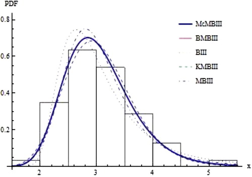
In this section we fit our purposed McMB-III distribution on real life data set. We fit the density functions of the McMB-III, MBIII, BIII, KMBIII and BMBIII distributions.

The first data set from Hussaini and Hussein [19] represent 64 observations for breaking strengths of single carbon fibres of length 10 are 1.901, 2.132, 2.203, 2.228, 2.257, 2.350, 2.361, 2.396, 2.397, 2.445, 2.614, 2.616, 2.618, 2.624, 2.659, 2.675, 2.532, 2.575, 2.454, 2.454, 2.474, 2.518, 2.522, 2.525, 2.738, 2.40, 2.856, 2.917, 2.928, 2.937, 2.937, 2.977, 2.996, 3.030, 3.125, 3.139, 3.145, 3.220, 3.223, 3.235, 3.243, 3.264, 3.272, 3.294, 3.332, 3.346, 3.377, 3.408, 3.435, 3.493, 3.501, 3.537, 3.554, 3.562, 3.628, 3.852, 3.871, 3.886, 3.971, 4.024, 4.027, 4.225, 4.395, 5.020.

The second data set of Average Annual Percent Change in Private Health Insurance Premiums from Kibria and Shakil [20] are 14.4, 14.0, 15.4, 9.4, 11.7, 15.0, 24.9, 20.7, 12.5, 14.9,12.6, 16.7, 13.8, 11.0, 12.9, 10.1, 1.9, 8.5, 16.5, 15.3,13.3, 9.8, 8.4, 7.9, 3.7, 5.1, 4.6, 4.4, 5.4, 6.1, 8.0, 10.0,11.2, 10.1, 6.4, 6.7, 5.7, 5.8

Estimates of the parameters of McMB-III distribution, Akaike Information Criterion (AIC), Consistent Akaike Information Criterion (AIC), Bayesian Information Criterion (BIC) and Hannan-Quinn Information Criterion are given in Table 2 for the first data set and in Table 3 for the second data set.

Table 2. Maximum Likelihood Estimator and Information Criterion for breaking strengths of single carbon fibres.

	MLE						Information Criterion
Model	$\alpha$	$\beta$	$\gamma$	$\lambda$	$\eta$	$\xi$	W	AIC	CAIC	HQIC
McMBIII	3.106	1.558	0.00	3.046	13.889	3.164	112.7	124.7	126.1	129.8
MBIII	2043.21	7.198	1025.1	1	1	1	124.9	130.9	131.3	133.45
BIII	233.77	5.44	1	1	1	1	127.8	131.8	131.99	133.50
BMBIII	5.92	1.141	0.0001	6.05	15.10	1	112.62	122.62	123.65	119.75
KMBIII	4.988	1.775	0.000	1	17.17	4.57	113.107	123.107	124.14	120.23

Table 3. Maximum Likelihood Estimator and Information Criterion Average Annual Percent Change in Private Health Insurance Premiums.

	MLE							Information Criterion
Model	$\alpha$	$\beta$	$\gamma$	$\lambda$	$\eta$	$\xi$	W	AIC	BIC	CAIC	HQIC
McMBIII	22.73	1.46	28.002	0.244	23.40	11.68	224.894	236.894	246.72	239.60	240.38
BIII	29.05	1.69	1	1	1	1	242.292	246.292	249.57	257.0	247.46
KMBIII	26.14	1.13	53.19	1	46.91	5.37	225.141	231.141	236.05	239.85	232.89

Figure 5 fitted densities for breaking strengths of single carbon fibres.

Figure 5. Histogram & fitted distribution.

Figure 6 fitted densities for Average Annual Percent Change in Private Health Insurance Premiums:

Figure 6. Histogram & fitted distribution.

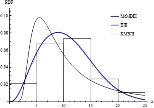
The McMBIII distribution gives the best fit than MBIII and BIII distributions. In Table 3 W is -2loglikelihood. The new sub-models, BMBIII and KMBIII, give less -2loglikelihood and information criterion as compared to our proposed model and old models. There are larger values of AIC, CAIC and HQIC for MBIII and BIII distribution as compared to McMB-III distribution. The McMB-III distribution gives the best fit than BIII distribution. In Table 3 W is -2loglikelihood. The new sub-model, KMBIII, give less -2loglikelihood and information criterion as compared to our proposed model and old models. There are larger values of AIC, BIC, CAIC and HQIC for BIII distribution as compared to McMB-III distribution.

The McMB-III distribution provides the close fit to a real data set. Thus our new distribution gives a better fit as compared to other sub models like Modified Burr-III and Burr-III distribution etc.

6. Conclusions

We have presented and developed the mathematical properties of a new class of distributions known as the McDonald modified Burr–III, including the hazard functions, moments, entropy, mean deviations, and maximum likelihood estimates. Two real data paradigms are presented to prove the application of the proposed model. The results show that our new model McMB–III is more flexible and yields the best fit compared to all the other submodels.

Acknowledgements

The Authors declare that there is no competing interest, and we are grateful to the anonymous reviewers for their valuable comments and suggestions in improving the manuscript.

Disclosure statement

No potential conflict of interest was reported by the authors.

ORCID

Samia Mukhtar http://orcid.org/0000-0001-9254-204X

Azeem Ali http://orcid.org/0000-0002-0042-2743

Al Mutairi Alya http://orcid.org/0000-0003-4181-6279

Appendix

Representing mode of MMB-III for different values of $\alpha ,\beta ,\gamma ,\lambda ,\eta ,\xi$.

Table

$\alpha =1,\beta =2,\gamma =1$
	$\xi =1$			$\xi =2$			$\xi =3$
Λ	$\eta =2$	$\eta =3$	$\eta =4$	$\eta =2$	$\eta =3$	$\eta =4$	$\eta =2$	$\eta =3$	$\eta =4$
1	0.45	0.38	0.33	0.85	0.76	0.71	1.12	1.02	0.96
2	0.77	0.65	0.56	1.24	1.10	1.0	1.58	1.41	1.30
3	1.0	0.84	0.74	1.54	1.34	1.21	1.93	1.70	1.55
4	1.18	1.0	0.88	1.78	1.54	1.39	2.23	1.94	1.76
5	1.34	1.13	1.0	1.99	1.72	1.54	2.48	2.15	1.95
6	1.48	1.25	1.11	2.18	1.88	1.68	2.71	2.35	2.11

Table

$\alpha =2,\beta =1,\gamma =1$
	$\xi =1$			$\xi =2$			$\xi =3$
Λ	$\eta =2$	$\eta =3$	$\eta =4$	$\eta =2$	$\eta =3$	$\eta =4$	$\eta =2$	$\eta =3$	$\eta =4$
1	0.41	0.35	0.32	1.28	1.15	1.05	2.16	1.95	1.81
2	1.12	0.91	0.78	2.71	2.28	2.01	4.30	3.66	3.25
3	1.80	1.44	1.21	4.08	3.34	2.88	6.36	5.25	4.56
4	2.47	1.95	1.63	5.43	4.37	3.72	8.39	6.80	5.83
5	3.14	2.46	2.04	6.78	5.39	4.55	10.41	8.34	7.07
6	3.81	2.96	2.45	8.12	6.14	5.37	12.43	9.86	8.30

Table

$\alpha =1,\beta =1,\gamma =2$
	$\xi =1$			$\xi =2$			$\xi =3$
Λ	$\eta =2$	$\eta =3$	$\eta =4$	$\eta =2$	$\eta =3$	$\eta =4$	$\eta =2$	$\eta =3$	$\eta =4$
1	–	–	–	0.0	0.0	0.4	0.39	0.33	0.71
2	–	–	–	0.67	0.5	0.4	1.44	1.15	1.82
3	0.25	0.15	0.09	1.33	1.0	0.8	2.46	1.93	2.87
4	0.56	0.36	0.25	2.0	1.5	1.2	3.47	2.69	3.90
5	0.88	0.59	0.42	2.67	2.0	1.6	4.47	3.45	4.92
6	1.21	0.82	0.60	3.33	2.5	2.0	5.48	4.21	5.93

Estimates, Log-Likelihood and p-values:

Table

Estimates	parameters	n = 50	n = 100	n = 150	n = 200
	0.5	1.1	0.4	0.5	0.6
	1.3	0.9	1.7	1.1	1.2
	1.7	0.5	0.6	1.7	1.75
	1.4	0.5	0.8	1.2	1.3
	0.65	0.6	0.4	0.7	0.6
	0.6	0.6	0.3	0.5	0.6
Log likelihood		−84	−172	−272	−280
P-values	Anderson-Darling	0.5	0.2	0.7	0.8
	Kolmogorov-Smirnov	0.6	0.4	0.6	0.7
	Pearson ${\chi }^2$	0.6	0.6	0.7	0.8

References

- Burr IW. Cumulative frequency functions. Ann Math Stat. 1942;13(2):215–232. doi: 10.1214/aoms/1177731607
- Gove JH, Ducey MJ, Leak WB, et al. Rotated sigmoid structures in managed uneven-aged northern hardwood stands: a look at the Burr Type III distribution. Forestry. 2008;81(2):161–176. doi: 10.1093/forestry/cpm025
- Lindsay SR, Wood GR, Woollons RC. Modelling the diameter distribution of forest stands using the Burr distribution. J Appl Stat. 1996;23(6):609–620. doi: 10.1080/02664769623973
- Nadarajah S, Kotz S. The beta exponential distribution. Reliab Eng Syst Saf. 2006;91(6):689–697. doi: 10.1016/j.ress.2005.05.008
- Nadarajah S, Kotz S. The beta Gumbel distribution. Math Probl Eng. 2004;2004(4):323–332. doi: 10.1155/S1024123X04403068
- Wingo DR. Maximum likelihood methods for fitting the Burr type XII distribution to multiply (progressively) censored life test data. Metrika. 1993;40(1):203–210. doi: 10.1007/BF02613681
- Wingo DR. Estimating the location of the Cauchy distribution by numerical global optimization. Commun Stat-Simul C. 1983;12(2):201–212. doi: 10.1080/03610918308812311
- Chernobai GB, Chesalov YA, Burgina EB, et al. Temperature effects on the IR spectra of crystalliine amino acids, dipeptides, and polyamino acids. I. Glycine. J Struct Chem. 2007;48(2):332–339. doi: 10.1007/s10947-007-0050-8
- Sherrick BJ, Garcia P, Tirupattur V. Recovering probabilistic information from option markets: Tests of distributional assumptions. J Futures Markets: Futures, Options, and Other Derivative Products. 1996;16(5):545–560. doi: 10.1002/(SICI)1096-9934(199608)16:5<545::AID-FUT3>3.0.CO;2-G
- Mielke PW, Jr. Another family of distributions for describing and analyzing precipitation data. J Appl Meteorol. 1973;12(2):275–280. doi: 10.1175/1520-0450(1973)012<0275:AFODFD>2.0.CO;2
- Tejeda HA, Goodwin BK. Modeling crop prices through a Burr distribution and analysis of correlation between crop prices and yields using a copula method. Annu Meeting Agr Appl Econ Assoc, Orlando, FL, USA. 2008;83(3):643–649.
- Abdel-Ghaly AA, Al-Dayian GR, Al-Kashkari FH. The use of burr type XII distribution on software reliability growth modelling. Microelectron Reliab. 1997;37(2):305–313. doi: 10.1016/0026-2714(95)00124-7
- Dagum C. New model of personal income-distribution-specification and estimation. Economie appliquée. 1977;30(3):413–437.
- Kleiber C, Kotz S. Statistical size distributions in economics and actuarial sciences. Vol. 470. Hoboken (NJ): John Wiley & Sons, Inc.; 2003.
- Shao Q, Chen YD, Zhang L. An extension of three-parameter Burr III distribution for low-flow frequency analysis. Comput Stat Data Anal. 2008;52(3):1304–1314. doi: 10.1016/j.csda.2007.06.014
- Syed AA. Anwer Hasnain and Munir Ahmad. “modified Burr-III distribution; properties and applications”. Pak J Stat. 2015;31(6):697–708.
- De Gusmao FR, Ortega EM, Cordeiro GM. The generalized inverse Weibull distribution. Stat Pap. 2011;52(3):591–619. doi: 10.1007/s00362-009-0271-3
- Shoukri MM, Mian IUH, Tracy DS. Sampling properties of estimators of the log-logistic distribution with application to Canadian precipitation data. Can J Stat. 1988;16(3):223–236. doi: 10.2307/3314729
- AL-Hussaini EK, Hussein M. Estimation using censored data from exponentiated Burr type XII population. Open J Stat. 2011;1(2):33–45. doi: 10.4236/ojs.2011.12005
- Kibria BG, Shakil M. A new five-parameter Burr system of distributions based on generalized Pearson differential equation. Proceedings, Section on Physical and Engineering Sciences; 2011.