Tension spline method for the solution of elliptic equations

Abstract

In this paper, two classes of methods are developed for the solution of two-dimensional elliptic partial differential equations. We have used tension spline function approximation in both x and y spatial directions and a new scheme of order $O(h^4+k^4)$ has been obtained. The convergence analysis of the methods has been carried out. Numerical examples are given to illustrate the applicability and accurate nature of our approach.

Keywords:

• Elliptic partial differential equation
• tension spline function
• iterative method
• convergence analysis

2010 MSC:

• 41A15
• 35J15

1. Introduction

Elliptic partial differential equations often arise in many fields of engineering and theoretical physics such as electric potential in electrostatics, electromagnetic scattering theory [1], micro and nano electronic devise physics, membrane vibration and radar scattering [2, 3].

We consider the linear second-order two-dimensional elliptic equation of the form (1) $A\frac{{\mathrm{\partial }}^{2}u}{\mathrm{\partial }{x}^2}+B\frac{{\mathrm{\partial }}^{2}u}{\mathrm{\partial }{y}^2}=Cu+f(x,y),(x,y)\in \mathrm{\Omega },$(1) subjected to Dirichlet boundary conditions $u(x,y)=g(x,y),(x,y)\in \mathrm{\partial \Omega },$ where A, B and C are positive constants and $\mathrm{\Omega }=\left\{\right(x,y);0<x,y<1\}$ with the boundary $\mathrm{\partial \Omega }$. We assume that the solution $u(x,y)$ and forcing function f are sufficiently smooth and have required continuous partial derivatives. The well-known Poisson equation and modified Helmholtz equation are special cases of Equation (1(1) $A\frac{{\mathrm{\partial }}^{2}u}{\mathrm{\partial }{x}^2}+B\frac{{\mathrm{\partial }}^{2}u}{\mathrm{\partial }{y}^2}=Cu+f(x,y),(x,y)\in \mathrm{\Omega },$(1) ).

Various numerical methods have been discussed and developed for solving elliptic partial differential equations. For the solution of two-dimensional Poisson equation, fourth-order compact difference schemes have discussed in [4, 5] and also a new family of high-order finite difference schemes is proposed in [6] by using implicit finite difference formulas. Sixth-order compact scheme is developed for the Poisson equation in [7] based on the fourth-order nine-point difference approximation, combined with Richardson extrapolation. Fourth-order finite difference methods for the solution of Helmholtz equation are presented in [8, 9]. Cubic spline collocation method was introduced for Poisson equation by Romenski [10]. Bialecki used orthogonal spline collocation method for the solution of Poisson equation [11]. The method of collocation at nodal points based on the tensor product of cubic splines for Helmholtz equation with Dirichlet boundary conditions was first analysed independently by Cavendish and Ito in their PhD theses and second-order convergence of the method was proved. Christara has developed quadratic spline collocation methods for elliptic problems in the unit square [12]. These methods which have third order of accuracy, collocate a perturbed differential equation. Houstis et al. analysed a new class of collocation methods using cubic spline for the general form of elliptic PDEs and derived fourth order of accuracy [13]. Quadratic spline collocation methods for two-dimensional Helmholtz problem are developed in [14], it is shown that the methods are fourth-order accurate at the nodes and collocation points. Rashidinia et al. proposed the cubic spline method for the singular elliptic boundary value problems in [15, 16]. Islam Khan et al. used tension spline method to solve second-order singularly perturbed boundary-value problems [17] also tension spline method for the solution of nonlinear partial differential equations have discussed in [18, 19]. Mohanty et al. have used a new finite difference scheme for two-dimensional elliptic problems [20], also they proposed cubic spline finite difference method of order $O(k^2+h^4)$ for two-dimensional quasi-linear elliptic equations [21]. Higher-order accurate finite volume schemes for two-dimensional Helmholtz equations are developed in [22]. For numerically solving inhomogeneous elliptic partial differential equations, a Chebyshev polynomial scheme combined with the method of fundamental solutions (MFS) and the equilibrated collocation Trefftz method have presented in [23] and a particular solution using the standard polynomial basis function has been derived in [24]. A new wavelet multigrid method based on Daubechies filter coefficients is proposed in [25] for the numerical solution of elliptic type equations.

In this paper, we have presented the non-polynomial tension spline method for two-dimensional linear elliptic equation (1(1) $A\frac{{\mathrm{\partial }}^{2}u}{\mathrm{\partial }{x}^2}+B\frac{{\mathrm{\partial }}^{2}u}{\mathrm{\partial }{y}^2}=Cu+f(x,y),(x,y)\in \mathrm{\Omega },$(1) ). We discussed the derivation of non-polynomial tension spline approximation and by using tension spline approximation in both spatial directions, two classes of nine-point scheme have been obtained. The truncation error of the scheme is carried out and convergence of our approach is proved.

2. Non-polynomial spline functions

We consider the solution domain $\mathrm{\Omega }=[0,1]\times [0,1]$ and choose grid spacing h>0 and k>0, in the x-direction and y-direction, respectively. The mesh points are defined by $(x_i,y_j)=(ih,jk)$, $i=0,1,\dots ,m+1,$ $j=0,1,\dots ,n+1$, where m and n are positive integers. In each segment $[x_i,x_{i+1}]$ let $s_{1j}\left(x\right)$ be the tension spline function which interpolates $u(x,y_j)$ and define (2) $\begin{array}{rl}{s}_{1j}\left(x\right)& =a_{1i}+b_{1i}(x-x_i)+c_{1i}\sinh {\lambda }_1(x-x_i)\\ & +d_{1i}\cosh {\lambda }_1(x-x_i),\end{array}$(2) where $a_{1i}$, $b_{1i}$, $c_{1i}$ and $d_{1i}$ are unknown coefficients and ${\lambda }_1$ is free parameter. Also, we let $s_{2i}\left(y\right)$ be the tension spline function interpolating $u(x_i,y_j)$ in each segment $[y_j,y_{j+1}]$ and define (3) $\begin{array}{rl}{s}_{2i}\left(y\right)& =a_{2j}+b_{2j}(y-y_j)+c_{2j}\sinh {\lambda }_2(y-y_j)\\ & +d_{2j}\cosh {\lambda }_2(y-y_j),\end{array}$(3) where $a_{2i}$, $b_{2i}$, $c_{2i}$ and $d_{2i}$ are unknown coefficients and ${\lambda }_2$ is an arbitrary parameter. To determine explicit expressions for all of coefficients we first denote (4) $\begin{array}{rl}{s}_{1j}\left(x_i\right)& =u_{i,j},s_{1j}\left(x_{i+1}\right)=u_{i+1,j},s_{2i}\left(y_j\right)=u_{i,j},\\ s_{2i}\left(y_{j+1}\right)& =u_{i,j+1},\end{array}$(4) (5) $\begin{array}{rl}{s}_{1j}^{\mathrm{\prime \prime }}\left(x_i\right)& =M_{1i,j},s_{1j}^{\mathrm{\prime \prime }}\left(x_{i+1}\right)=M_{1i+1,j},\\ s_{2i}^{\mathrm{\prime \prime }}\left(y_j\right)& =M_{2i,j},s_{2i}^{\mathrm{\prime \prime }}\left(y_{j+1}\right)=M_{2i,j+1}.\end{array}$(5) By using (4(4) $\begin{array}{rl}{s}_{1j}\left(x_i\right)& =u_{i,j},s_{1j}\left(x_{i+1}\right)=u_{i+1,j},s_{2i}\left(y_j\right)=u_{i,j},\\ s_{2i}\left(y_{j+1}\right)& =u_{i,j+1},\end{array}$(4) ) and (5(5) $\begin{array}{rl}{s}_{1j}^{\mathrm{\prime \prime }}\left(x_i\right)& =M_{1i,j},s_{1j}^{\mathrm{\prime \prime }}\left(x_{i+1}\right)=M_{1i+1,j},\\ s_{2i}^{\mathrm{\prime \prime }}\left(y_j\right)& =M_{2i,j},s_{2i}^{\mathrm{\prime \prime }}\left(y_{j+1}\right)=M_{2i,j+1}.\end{array}$(5) ) and from algebraic manipulations we derive $\begin{array}{rl}{a}_{1i}& =u_{i,j}-\frac{1}{{\lambda }_1^2{M}_{1i,j}},b_{1i}=\frac{1}{h}(u_{i+1,j}-u_{i,j})\\ & +\frac{1}{{\omega }_1{\lambda }_1}(M_{1i,j}-M_{1i+1,j}),\\ c_{1i}& =\frac{1}{{\lambda }_1^2}\left(\mathrm{csch}\right({\omega }_1)M_{1i+1,j}-\coth ({\omega }_1\left)M_{1i,j}\right),\\ d_{1i}& =\frac{1}{{\lambda }_1^2}{M}_{1i,j},\end{array}$ where ${\omega }_1={\lambda }_{1}h.$ And also $\begin{array}{rl}{a}_{2j}& =u_{i,j}-\frac{1}{{\lambda }_2^2}{M}_{2i,j},b_{2j}=\frac{1}{k}(u_{i,j+1}-u_{i,j})\\ & +\frac{1}{{\omega }_2{\lambda }_2}(M_{2i,j}-M_{2i,j+1}),\\ c_{2j}& =\frac{1}{{\lambda }_2^2}\left(\mathrm{csch}\right({\omega }_2)M_{2i,j+1}-\coth ({\omega }_2\left)M_{2i,j}\right),\\ d_{2j}& =\frac{1}{{\lambda }_2^2}{M}_{2i,j},\end{array}$ where ${\omega }_2={\lambda }_{2}k.$

From the continuity of the first derivatives of spline functions $s_{1j}\left(x\right)$ and $s_{2i}\left(y\right)$ at $(x_i,y_j),$ we get the following consistency relations: (6) $\begin{array}{rl}& \frac{1}{h^2}(u_{i-1,j}-2u_{i,j}+u_{i+1,j})\\ & ={\alpha }_1{M}_{1i-1,j}+2{\beta }_1{M}_{1i,j}+{\alpha }_1{M}_{1i+1,j},\end{array}$(6) (7) $\begin{array}{rl}& \frac{1}{k^2}(u_{i,j-1}-2u_{i,j}+u_{i,j+1})\\ & ={\alpha }_2{M}_{2i,j-1}+2{\beta }_2{M}_{2i,j}+{\alpha }_2{M}_{2i,j+1},\end{array}$(7) where $\begin{array}{rl}{\alpha }_1& =\frac{1}{{\omega }_1^2}(1-{\omega }_1\mathrm{csch}({\omega }_1\left)\right),\\ {\beta }_1& =\frac{1}{{\omega }_1^2}({\omega }_1\coth ({\omega }_1)-1),\\ {\alpha }_2& =\frac{1}{{\omega }_2^2}(1-{\omega }_2\mathrm{csch}({\omega }_2\left)\right),\\ {\beta }_2& =\frac{1}{{\omega }_2^2}({\omega }_2\coth ({\omega }_2)-1).\end{array}$ When ${\lambda }_1\to 0$ that ${\omega }_1\to 0$,then $({\alpha }_1,{\beta }_1)\to (1/6,1/3)$ and also when ${\lambda }_2\to 0$, then $({\alpha }_2,{\beta }_2)\to (1/6,1/3)$ so consistency relations of tension splines defined in (6(6) $\begin{array}{rl}& \frac{1}{h^2}(u_{i-1,j}-2u_{i,j}+u_{i+1,j})\\ & ={\alpha }_1{M}_{1i-1,j}+2{\beta }_1{M}_{1i,j}+{\alpha }_1{M}_{1i+1,j},\end{array}$(6) ) and (7(7) $\begin{array}{rl}& \frac{1}{k^2}(u_{i,j-1}-2u_{i,j}+u_{i,j+1})\\ & ={\alpha }_2{M}_{2i,j-1}+2{\beta }_2{M}_{2i,j}+{\alpha }_2{M}_{2i,j+1},\end{array}$(7) ) reduce to the following cubic spline relations, respectively: (8) $\begin{array}{r}(u_{i-1,j}-2u_{i,j}+u_{i+1,j})=\frac{h^2}{6}(M_{1i-1,j}+4M_{1i,j}+M_{1i+1,j}),\end{array}$(8) (9) $\begin{array}{r}(u_{i,j-1}-2u_{i,j}+u_{i,j+1})=\frac{k^2}{6}(M_{2i,j-1}+4M_{2i,j}+M_{2i,j+1}).\end{array}$(9)

3. Spline numerical methods

At the grid point $(x_i,y_j)$, Equation (1(1) $A\frac{{\mathrm{\partial }}^{2}u}{\mathrm{\partial }{x}^2}+B\frac{{\mathrm{\partial }}^{2}u}{\mathrm{\partial }{y}^2}=Cu+f(x,y),(x,y)\in \mathrm{\Omega },$(1) ) may be discretized as (10) $A{u}_{xx}(x_i,y_j)+B{u}_{yy}(x_i,y_j)=Cu(x_i,y_j)+f(x_i,y_j).$(10) We next develop an approximation for Equation (1(1) $A\frac{{\mathrm{\partial }}^{2}u}{\mathrm{\partial }{x}^2}+B\frac{{\mathrm{\partial }}^{2}u}{\mathrm{\partial }{y}^2}=Cu+f(x,y),(x,y)\in \mathrm{\Omega },$(1) ) in which we use the non-polynomial tension spline functions approximations of second derivatives in x-direction and also in y-direction: (11) $\begin{array}{r}{u}_{xx}(x_i,y_j)\cong M_{1i,j},\end{array}$(11) (12) $\begin{array}{r}{u}_{yy}(x_i,y_j)\cong M_{2i,j}.\end{array}$(12) From (10(10) $A{u}_{xx}(x_i,y_j)+B{u}_{yy}(x_i,y_j)=Cu(x_i,y_j)+f(x_i,y_j).$(10) ) and by neglecting the truncation error, we get (13) $\begin{array}{r}A{M}_{1i,j}+B{M}_{2i,j}=C{u}_{i,j}+f_{i,j},\end{array}$(13) (14) $\begin{array}{r}A{M}_{1i\underset{\_}{+}1,j}+B{M}_{2i\underset{\_}{+}1,j}=C{u}_{i\underset{\_}{+}1,j}+f_{i\underset{\_}{+}1,j},\end{array}$(14) (15) $\begin{array}{r}A{M}_{1i,j\underset{\_}{+}1}+B{M}_{2i,j\underset{\_}{+}1}=C{u}_{i,j\underset{\_}{+}1}+f_{i,j\underset{\_}{+}1}.\end{array}$(15) Similar to (6(6) $\begin{array}{rl}& \frac{1}{h^2}(u_{i-1,j}-2u_{i,j}+u_{i+1,j})\\ & ={\alpha }_1{M}_{1i-1,j}+2{\beta }_1{M}_{1i,j}+{\alpha }_1{M}_{1i+1,j},\end{array}$(6) ), for the $(j-1)$-th and $(j+1)$-th levels in y-direction we have (16) $\begin{array}{rl}& (u_{i-1,j-1}-2u_{i,j-1}+u_{i+1,j-1})\\ & =h^2({\alpha }_1{M}_{1i-1,j-1}+2{\beta }_1{M}_{1i,j-1}+{\alpha }_1{M}_{1i+1,j-1}),\end{array}$(16) (17) $\begin{array}{rl}& (u_{i-1,j+1}-2u_{i,j+1}+u_{i+1,j+1})\\ & =h^2({\alpha }_1{M}_{1i-1,j+1}+2{\beta }_1{M}_{1i,j+1}+{\alpha }_1{M}_{1i+1,j+1}).\end{array}$(17) Similar to (7(7) $\begin{array}{rl}& \frac{1}{k^2}(u_{i,j-1}-2u_{i,j}+u_{i,j+1})\\ & ={\alpha }_2{M}_{2i,j-1}+2{\beta }_2{M}_{2i,j}+{\alpha }_2{M}_{2i,j+1},\end{array}$(7) ), for the $(i-1)$-th and $(i+1)$-th levels in x-direction we have (18) $\begin{array}{rl}& (u_{i-1,j-1}-2u_{i-1,j}+u_{i-1,j+1})\\ & =k^2({\alpha }_2{M}_{2i-1,j-1}+2{\beta }_2{M}_{2i-1,j}+{\alpha }_2{M}_{2i-1,j+1}),\end{array}$(18) (19) $\begin{array}{rl}& (u_{i+1,j-1}-2u_{i+1,j}+u_{i+1,j+1})\\ & =k^2({\alpha }_2{M}_{2i+1,j-1}+2{\beta }_2{M}_{2i+1,j}+{\alpha }_2{M}_{2i+1,j+1}).\end{array}$(19) By using Equations (6(6) $\begin{array}{rl}& \frac{1}{h^2}(u_{i-1,j}-2u_{i,j}+u_{i+1,j})\\ & ={\alpha }_1{M}_{1i-1,j}+2{\beta }_1{M}_{1i,j}+{\alpha }_1{M}_{1i+1,j},\end{array}$(6) ), (7(7) $\begin{array}{rl}& \frac{1}{k^2}(u_{i,j-1}-2u_{i,j}+u_{i,j+1})\\ & ={\alpha }_2{M}_{2i,j-1}+2{\beta }_2{M}_{2i,j}+{\alpha }_2{M}_{2i,j+1},\end{array}$(7) ) and (13(13) $\begin{array}{r}A{M}_{1i,j}+B{M}_{2i,j}=C{u}_{i,j}+f_{i,j},\end{array}$(13) )–(19(19) $\begin{array}{rl}& (u_{i+1,j-1}-2u_{i+1,j}+u_{i+1,j+1})\\ & =k^2({\alpha }_2{M}_{2i+1,j-1}+2{\beta }_2{M}_{2i+1,j}+{\alpha }_2{M}_{2i+1,j+1}).\end{array}$(19) ) and after manipulating them we obtain (20) $\begin{array}{rl}& p_1(u_{i-1,j-1}+u_{i-1,j+1}+u_{i+1,j-1}+u_{i+1,j+1})\\ & +p_2(u_{i-1,j}+u_{i+1,j})+p_3(u_{i,j-1}+u_{i,j+1})+p_4{u}_{i,j}\\ & =r_1(f_{i-1,j-1}+f_{i-1,j+1}+f_{i+1,j-1}+f_{i+1,j+1})\\ & +r_2(f_{i-1,j}+f_{i+1,j})+r_3(f_{i,j-1}+f_{i,j+1})+r_4{f}_{i,j},\end{array}$(20) where (21) $\begin{array}{rl}{p}_1& =A{k}^2{\alpha }_2+B{h}^2{\alpha }_1-C{r}_1,\\ p_2& =2A{k}^2{\beta }_2-2B{h}^2{\alpha }_1-C{r}_2,\\ p_3& =2B{h}^2{\beta }_1-2A{k}^2{\alpha }_2-C{r}_3,\\ p_4& =-4A{k}^2{\beta }_2-4B{h}^2{\beta }_1-C{r}_4,\end{array}$(21) (22) $\begin{array}{rl}{r}_1& =h^2{k}^2{\alpha }_1{\alpha }_2,r_2=2h^2{k}^2{\alpha }_1{\beta }_2,\\ r_3& =2h^2{k}^2{\alpha }_2{\beta }_1,r_4=4h^2{k}^2.{\beta }_1{\beta }_2\end{array}$(22)

4. Truncation error

The partial differential equation (10(10) $A{u}_{xx}(x_i,y_j)+B{u}_{yy}(x_i,y_j)=Cu(x_i,y_j)+f(x_i,y_j).$(10) ) may be discretized as (23) $f_{i,j}=(A{D}_x^2+B{D}_y^2-C)u_{i,j},$(23) where $D_x^2=\left({\mathrm{\partial }}^2/\mathrm{\partial }{x}^2\right)$ and $D_y^2=\left({\mathrm{\partial }}^2/\mathrm{\partial }{y}^2\right).$ Also we have $\begin{array}{rl}& f_{i\underset{\_}{+}1,j}=(A{D}_x^2+B{D}_y^2-C)u_{i\underset{\_}{+}1,j},\\ & f_{i,j\underset{\_}{+}1}=(A{D}_x^2+B{D}_y^2-C)u_{i,j\underset{\_}{+}1}.\end{array}$ Now,by using the above notations and expanding both sides of (20(20) $\begin{array}{rl}& p_1(u_{i-1,j-1}+u_{i-1,j+1}+u_{i+1,j-1}+u_{i+1,j+1})\\ & +p_2(u_{i-1,j}+u_{i+1,j})+p_3(u_{i,j-1}+u_{i,j+1})+p_4{u}_{i,j}\\ & =r_1(f_{i-1,j-1}+f_{i-1,j+1}+f_{i+1,j-1}+f_{i+1,j+1})\\ & +r_2(f_{i-1,j}+f_{i+1,j})+r_3(f_{i,j-1}+f_{i,j+1})+r_4{f}_{i,j},\end{array}$(20) ) in Taylor series in terms of $u(x_i,y_j)$ and its derivatives, we obtain the truncation error of the method as follows: (24) $\begin{array}{rl}{T}_{i,j}& =\left[\phantom{\frac{1}{12}{\alpha }_2\left(\frac{1}{30}-{\alpha }_1\right)}2({\alpha }_2+{\beta }_2)(1-2{\alpha }_1-2{\beta }_1)A{h}^2{k}^2{D}_x^2\right.\\ & +2({\alpha }_1+{\beta }_1)(1-2{\alpha }_2-2{\beta }_2)B{h}^2{k}^2{D}_y^2\\ & +{\alpha }_2(1-2{\alpha }_1-2{\beta }_1)A{h}^2{k}^4{D}_x^2{D}_y^2\\ & +{\alpha }_1(1-2{\alpha }_2-2{\beta }_2)B{h}^4{k}^2{D}_x^2{D}_y^2\\ & +2\left(\frac{1}{12}-{\alpha }_1\right)({\alpha }_2+{\beta }_2)A{h}^4{k}^2{D}_x^4\\ & +2\left(\frac{1}{12}-{\alpha }_2\right)({\alpha }_1+{\beta }_1)B{h}^2{k}^4{D}_y^4\\ & +{\alpha }_2\left(\frac{1}{12}-{\alpha }_1\right)A{h}^4{k}^4{D}_x^4{D}_y^2\\ & +{\alpha }_1\left(\frac{1}{12}-{\alpha }_2\right)2{\beta }_{1}B{h}^4{k}^4{D}_x^2{D}_y^4\\ & +\frac{1}{12}{\alpha }_2(1-2{\alpha }_1-2{\beta }_1)A{h}^2{k}^6{D}_x^2{D}_y^4\\ & +\frac{1}{12}{\alpha }_1(1-2{\alpha }_2-2{\beta }_2)B{h}^6{k}^2{D}_x^4{D}_y^2\\ & +\frac{1}{6}\left(\frac{1}{30}-{\alpha }_1\right)({\alpha }_2+{\beta }_2)A{h}^6{k}^2{D}_x^6\\ & +\frac{1}{6}\left(\frac{1}{30}-{\alpha }_2\right)({\alpha }_1+{\beta }_1)B{h}^2{k}^6{D}_y^6\\ & +\frac{1}{360}{\alpha }_2(1-2{\alpha }_1-2{\beta }_1)A{h}^2{k}^8{D}_x^2{D}_y^6\\ & +\frac{1}{360}{\alpha }_1(1-2{\alpha }_2-2{\beta }_2)B{h}^8{k}^2{D}_x^6{D}_y^2\\ & +\frac{1}{12}{\alpha }_2\left(\frac{1}{30}-{\alpha }_1\right)A{h}^6{k}^4{D}_x^6{D}_y^2\\ & +\frac{1}{12}{\alpha }_1\left(\frac{1}{30}-{\alpha }_2\right)B{h}^4{k}^6{D}_x^2{D}_y^6\\ & +\frac{1}{12}{\alpha }_2\left(\frac{1}{30}-{\alpha }_1\right)A{h}^4{k}^6{D}_x^4{D}_y^4\\ & \left.+\frac{1}{12}{\alpha }_1\left(\frac{1}{30}-{\alpha }_2\right)B{h}^6{k}^4{D}_x^4{D}_y^4+\cdots \right]u_{i,j}.\end{array}$(24) From (24(24) $\begin{array}{rl}{T}_{i,j}& =\left[\phantom{\frac{1}{12}{\alpha }_2\left(\frac{1}{30}-{\alpha }_1\right)}2({\alpha }_2+{\beta }_2)(1-2{\alpha }_1-2{\beta }_1)A{h}^2{k}^2{D}_x^2\right.\\ & +2({\alpha }_1+{\beta }_1)(1-2{\alpha }_2-2{\beta }_2)B{h}^2{k}^2{D}_y^2\\ & +{\alpha }_2(1-2{\alpha }_1-2{\beta }_1)A{h}^2{k}^4{D}_x^2{D}_y^2\\ & +{\alpha }_1(1-2{\alpha }_2-2{\beta }_2)B{h}^4{k}^2{D}_x^2{D}_y^2\\ & +2\left(\frac{1}{12}-{\alpha }_1\right)({\alpha }_2+{\beta }_2)A{h}^4{k}^2{D}_x^4\\ & +2\left(\frac{1}{12}-{\alpha }_2\right)({\alpha }_1+{\beta }_1)B{h}^2{k}^4{D}_y^4\\ & +{\alpha }_2\left(\frac{1}{12}-{\alpha }_1\right)A{h}^4{k}^4{D}_x^4{D}_y^2\\ & +{\alpha }_1\left(\frac{1}{12}-{\alpha }_2\right)2{\beta }_{1}B{h}^4{k}^4{D}_x^2{D}_y^4\\ & +\frac{1}{12}{\alpha }_2(1-2{\alpha }_1-2{\beta }_1)A{h}^2{k}^6{D}_x^2{D}_y^4\\ & +\frac{1}{12}{\alpha }_1(1-2{\alpha }_2-2{\beta }_2)B{h}^6{k}^2{D}_x^4{D}_y^2\\ & +\frac{1}{6}\left(\frac{1}{30}-{\alpha }_1\right)({\alpha }_2+{\beta }_2)A{h}^6{k}^2{D}_x^6\\ & +\frac{1}{6}\left(\frac{1}{30}-{\alpha }_2\right)({\alpha }_1+{\beta }_1)B{h}^2{k}^6{D}_y^6\\ & +\frac{1}{360}{\alpha }_2(1-2{\alpha }_1-2{\beta }_1)A{h}^2{k}^8{D}_x^2{D}_y^6\\ & +\frac{1}{360}{\alpha }_1(1-2{\alpha }_2-2{\beta }_2)B{h}^8{k}^2{D}_x^6{D}_y^2\\ & +\frac{1}{12}{\alpha }_2\left(\frac{1}{30}-{\alpha }_1\right)A{h}^6{k}^4{D}_x^6{D}_y^2\\ & +\frac{1}{12}{\alpha }_1\left(\frac{1}{30}-{\alpha }_2\right)B{h}^4{k}^6{D}_x^2{D}_y^6\\ & +\frac{1}{12}{\alpha }_2\left(\frac{1}{30}-{\alpha }_1\right)A{h}^4{k}^6{D}_x^4{D}_y^4\\ & \left.+\frac{1}{12}{\alpha }_1\left(\frac{1}{30}-{\alpha }_2\right)B{h}^6{k}^4{D}_x^4{D}_y^4+\cdots \right]u_{i,j}.\end{array}$(24) ) we conclude that

• If we choose (25) $\begin{array}{rl}& {\alpha }_1+{\beta }_1=\frac{1}{2},{\alpha }_2+{\beta }_2=\frac{1}{2},\\ & {\alpha }_1\ne \frac{1}{12},{\alpha }_2\ne \frac{1}{12},\end{array}$(25) we obtain various schemes of order $O(h^2+k^2)$. In particular we can choose ${\alpha }_1={\alpha }_2=\left(1/6\right)$ and ${\beta }_1={\beta }_2=\left(1/3\right)$, which we denoted this scheme by $T_1$.

• If we choose (26) $\begin{array}{rl}& {\alpha }_1+{\beta }_1=\frac{1}{2},{\alpha }_2+{\beta }_2=\frac{1}{2},{\alpha }_1=\frac{1}{12},\\ & {\beta }_1=\frac{5}{12},{\alpha }_2=\frac{1}{12},{\beta }_2=\frac{5}{12},\end{array}$(26) we get a new scheme of $O(h^4+k^4)$, which we denoted by $T_2.$

5. Convergence analysis

The scheme (20(20) $\begin{array}{rl}& p_1(u_{i-1,j-1}+u_{i-1,j+1}+u_{i+1,j-1}+u_{i+1,j+1})\\ & +p_2(u_{i-1,j}+u_{i+1,j})+p_3(u_{i,j-1}+u_{i,j+1})+p_4{u}_{i,j}\\ & =r_1(f_{i-1,j-1}+f_{i-1,j+1}+f_{i+1,j-1}+f_{i+1,j+1})\\ & +r_2(f_{i-1,j}+f_{i+1,j})+r_3(f_{i,j-1}+f_{i,j+1})+r_4{f}_{i,j},\end{array}$(20) ) may be written in the following matrix form: (27) $PU=F,$(27) where U is the solution vector in the form $U={[u_{1,1},u_{2,1},\dots ,u_{m,1},\dots ,u_{1,n},u_{2,n},\dots ,u_{m,n}]}^{\mathrm{T}}$ and F is the right-hand side vector. P is a square block tridiagonal matrix of order $n\times n$ and can be expressed as P=L+D+R, where D is block diagonal matrix which each block of D is a triangular matrix in the form $tri[p_2,p_4,p_2].$ L and R are strictly block lower triangular and strictly block upper triangular matrices, respectively. The blocks of R and L are equals to each other and are in the form $tri[p_1,p_3,p_1]$, where the triangular matrix $T=tri[a,b,a]$ is defined by $T=\left(t_{ij}\right)=\left\{\begin{array}{ll}b,& i=j,\\ a,& \mid i-j\mid =1,\\ 0& \mathrm{otherwise}.\end{array}\right.$ From relations (21(21) $\begin{array}{rl}{p}_1& =A{k}^2{\alpha }_2+B{h}^2{\alpha }_1-C{r}_1,\\ p_2& =2A{k}^2{\beta }_2-2B{h}^2{\alpha }_1-C{r}_2,\\ p_3& =2B{h}^2{\beta }_1-2A{k}^2{\alpha }_2-C{r}_3,\\ p_4& =-4A{k}^2{\beta }_2-4B{h}^2{\beta }_1-C{r}_4,\end{array}$(21) ) and (22(22) $\begin{array}{rl}{r}_1& =h^2{k}^2{\alpha }_1{\alpha }_2,r_2=2h^2{k}^2{\alpha }_1{\beta }_2,\\ r_3& =2h^2{k}^2{\alpha }_2{\beta }_1,r_4=4h^2{k}^2.{\beta }_1{\beta }_2\end{array}$(22) ) we have $\begin{array}{rl}|p_1|& =|C{r}_1-A{k}^2{\alpha }_2-B{h}^2{\alpha }_1|\le C{r}_1,\\ |p_2|& \le 2A{k}^2{\beta }_2,|p_3|\le 2B{h}^2{\beta }_1.\end{array}$ Then using (25(25) $\begin{array}{rl}& {\alpha }_1+{\beta }_1=\frac{1}{2},{\alpha }_2+{\beta }_2=\frac{1}{2},\\ & {\alpha }_1\ne \frac{1}{12},{\alpha }_2\ne \frac{1}{12},\end{array}$(25) ) and (26(26) $\begin{array}{rl}& {\alpha }_1+{\beta }_1=\frac{1}{2},{\alpha }_2+{\beta }_2=\frac{1}{2},{\alpha }_1=\frac{1}{12},\\ & {\beta }_1=\frac{5}{12},{\alpha }_2=\frac{1}{12},{\beta }_2=\frac{5}{12},\end{array}$(26) ) we can obtain $\begin{array}{rl}& \left(\mathrm{i}\right)2|p_1|+|p_2|+2|p_3|<|p_4|,\end{array}$ (28) $\begin{array}{rl}& \left(\mathrm{iii}\right)2|p_1|+2|p_2|+|p_3|<|p_4|,\\ & \left(\mathrm{iv}\right)4|p_1|+2|p_2|+2|p_3|<|p_4|.\end{array}$(28) From (28(28) $\begin{array}{rl}& \left(\mathrm{iii}\right)2|p_1|+2|p_2|+|p_3|<|p_4|,\\ & \left(\mathrm{iv}\right)4|p_1|+2|p_2|+2|p_3|<|p_4|.\end{array}$(28) ) we conclude that P is a diagonally dominant matrix and the system (27(27) $PU=F,$(27) ) has unique solution. For solving the system (27(27) $PU=F,$(27) ) by P=L+D+R, the block Jacobi method is as follows: $U^{(n+1)}=M_J{U}^{\left(n\right)}+D^{-1}f,$ where $M_J$, the Jacobi iteration matrix is defined by $M_J=-D^{-1}(L+R)$. Also the block Gauss–Seidel method is $U^{(n+1)}=M_{GS}{U}^{\left(n\right)}+{(L+D)}^{-1}f,$ where $M_{GS}=-{(L+D)}^{-1}R.$

For the nine-point scheme (20(20) $\begin{array}{rl}& p_1(u_{i-1,j-1}+u_{i-1,j+1}+u_{i+1,j-1}+u_{i+1,j+1})\\ & +p_2(u_{i-1,j}+u_{i+1,j})+p_3(u_{i,j-1}+u_{i,j+1})+p_4{u}_{i,j}\\ & =r_1(f_{i-1,j-1}+f_{i-1,j+1}+f_{i+1,j-1}+f_{i+1,j+1})\\ & +r_2(f_{i-1,j}+f_{i+1,j})+r_3(f_{i,j-1}+f_{i,j+1})+r_4{f}_{i,j},\end{array}$(20) ) the Jacobi iteration formula is (29) $\begin{array}{rl}{u}_{i,j}^{(n+1)}& =\frac{-1}{p_4}\left[p_1\right(u_{i-1,j-1}^{\left(n\right)}+u_{i-1,j+1}^{\left(n\right)}+u_{i+1,j-1}^{\left(n\right)}\\ & +u_{i+1,j+1}^{\left(n\right)})+p_2(u_{i-1,j}^{\left(n\right)}+u_{i+1,j}^{\left(n\right)})\\ & +p_3(u_{i,j-1}^{\left(n\right)}+u_{i,j+1}^{\left(n\right)})]\\ & +\frac{1}{p_4}\left[r_1\right(f_{i-1,j-1}+f_{i-1,j+1}+f_{i+1,j-1}+f_{i+1,j+1})\\ & +r_2(f_{i-1,j}+f_{i+1,j})+r_3(f_{i,j-1}+f_{i,j+1})+r_4{f}_{i,j}].\end{array}$(29) The error equation of the iteration is (30) $\begin{array}{rl}{\epsilon }_{i,j}^{(n+1)}& =\frac{-1}{p_4}\left(p_1\right({\epsilon }_{i-1,j-1}^{\left(n\right)}+{\epsilon }_{i-1,j+1}^{\left(n\right)}+{\epsilon }_{i+1,j-1}^{\left(n\right)}+{\epsilon }_{i+1,j+1}^{\left(n\right)})\\ & +p_2({\epsilon }_{i-1,j}^{\left(n\right)}+{\epsilon }_{i+1,j}^{\left(n\right)})+p_3({\epsilon }_{i,j-1}^{\left(n\right)}+{\epsilon }_{i,j+1}^{\left(n\right)})),\end{array}$(30) where the values of the error are equal to zero on the boundary of the unit square.

Equation (30(30) $\begin{array}{rl}{\epsilon }_{i,j}^{(n+1)}& =\frac{-1}{p_4}\left(p_1\right({\epsilon }_{i-1,j-1}^{\left(n\right)}+{\epsilon }_{i-1,j+1}^{\left(n\right)}+{\epsilon }_{i+1,j-1}^{\left(n\right)}+{\epsilon }_{i+1,j+1}^{\left(n\right)})\\ & +p_2({\epsilon }_{i-1,j}^{\left(n\right)}+{\epsilon }_{i+1,j}^{\left(n\right)})+p_3({\epsilon }_{i,j-1}^{\left(n\right)}+{\epsilon }_{i,j+1}^{\left(n\right)})),\end{array}$(30) ) can be solved by the method of separation of variables, we let (31) $\begin{array}{r}{\epsilon }_{i,j}^{\left(n\right)}=V_i.W_j,\end{array}$(31) (32) $\begin{array}{r}{\epsilon }_{i,j}^{(n+1)}=\xi {\epsilon }_{i,j}^{\left(n\right)},\end{array}$(32) where ξ is the propagation factor.By substituting (31(31) $\begin{array}{r}{\epsilon }_{i,j}^{\left(n\right)}=V_i.W_j,\end{array}$(31) ) and (32(32) $\begin{array}{r}{\epsilon }_{i,j}^{(n+1)}=\xi {\epsilon }_{i,j}^{\left(n\right)},\end{array}$(32) ) in (30(30) $\begin{array}{rl}{\epsilon }_{i,j}^{(n+1)}& =\frac{-1}{p_4}\left(p_1\right({\epsilon }_{i-1,j-1}^{\left(n\right)}+{\epsilon }_{i-1,j+1}^{\left(n\right)}+{\epsilon }_{i+1,j-1}^{\left(n\right)}+{\epsilon }_{i+1,j+1}^{\left(n\right)})\\ & +p_2({\epsilon }_{i-1,j}^{\left(n\right)}+{\epsilon }_{i+1,j}^{\left(n\right)})+p_3({\epsilon }_{i,j-1}^{\left(n\right)}+{\epsilon }_{i,j+1}^{\left(n\right)})),\end{array}$(30) ), we get (33) $W_{j-1}-\gamma W_j+W_{j+1}=0$(33) and (34) $l_1{V}_{i-1}+l_2{V}_i+l_1{V}_{i+1}=0,$(34) where γ is an arbitrary parameter to be determine and (35) $l_1=p_1\gamma +p_2,l_2=p_3\gamma +p_4\xi ,$(35) and boundary conditions are $V_0=V_{m+1}=0$ and $W_0=W_{n+1}=0$.

The solution of difference equation (33(33) $W_{j-1}-\gamma W_j+W_{j+1}=0$(33) ) subject to homogeneous boundary conditions is (36) $W_j=w_1\sin \left(k\pi qj\right),1\le j\le n,1\le q\le n$(36) with $\gamma =2\cos \left(k\pi q\right)$ and $w_1$ an arbitrary constant.

Also, the solution of (34(34) $l_1{V}_{i-1}+l_2{V}_i+l_1{V}_{i+1}=0,$(34) ) with homogeneous boundary conditions is (37) $\begin{array}{rl}{V}_i& =v_1\sin \left(h\pi pi\right),1\le i\le m,1\le p\le m,\end{array}$(37) (38) $\begin{array}{rl}{l}_2& =-2l_1\cos \left(h\pi p\right),\end{array}$(38) and $v_1$ is an arbitrary constant. By eliminating $l_1$ and $l_2$ from (35(35) $l_1=p_1\gamma +p_2,l_2=p_3\gamma +p_4\xi ,$(35) ) and (38(38) $\begin{array}{rl}{l}_2& =-2l_1\cos \left(h\pi p\right),\end{array}$(38) ), we get (39) $\begin{array}{rl}\xi & =\frac{1}{p_4}(-4p_1\cos (k\pi q)\cos (h\pi p)-2p_2\cos (h\pi p)\\ & -2p_3\cos \left(k\pi q\right)).\end{array}$(39) From (28(28) $\begin{array}{rl}& \left(\mathrm{iii}\right)2|p_1|+2|p_2|+|p_3|<|p_4|,\\ & \left(\mathrm{iv}\right)4|p_1|+2|p_2|+2|p_3|<|p_4|.\end{array}$(28) -(iv)) and (39(39) $\begin{array}{rl}\xi & =\frac{1}{p_4}(-4p_1\cos (k\pi q)\cos (h\pi p)-2p_2\cos (h\pi p)\\ & -2p_3\cos \left(k\pi q\right)).\end{array}$(39) ), we conclude that $|\xi |<1.$ Therefore, the Jacobi method converges for any initial guess and for any values of h and k. Also the spectral radius ρ of Jacobi and Gauss–Seidel iteration matrices are related by $\rho \left(M_{GS}\right)={\rho \left(M_J\right)}^2.$ Thus the Gauss–Seidel method converges too.

6. Numerical results

In this section, we consider the following examples with the known exact solutions. We applied our methods to solve these examples, with various values of h and k. The computed solutions at grid points are compared with the exact solutions, the maximum absolute errors and convergence orders are tabulated in Tables 1–3.The orders of convergence are established from the following relation:

Table 1. The maximum absolute errors and orders of convergence of Example 6.1.

(h,k)	Method ($T_1$)	Conv. order	Method ($T_2$)	Conv. order
(1/16, 1/16)	2.4162 E−3		6.6144 E−6
(1/16, 1/32)	2.0264 E−3		5.6684 E−6
(1/32, 1/16)	9.9654 E−4		1.3588 E−6
(1/32, 1/32)	6.0505 E−4	1.99	4.1319 E−7	4.00
(1/64, 1/64)	1.4752 E−4	2.04	2.5170 E−8	4.04
(1/128, 1/128)	2.3373 E−5	2.66	9.8365 E−10	4.67

Table 2. The maximum absolute errors in Example 6.2.

(h,k)	Our method ($T_2$)	Conv. order	Method [13]	Conv. order
(1/6, 1/6)	2.315 E−5	–	5.72 E−3	–
(1/9, 1/9)	4.758 E−6	3.90	8.29 E−4	4.11
(1/17, 1/17)	3.714 E−7	4.01	5.89 E−5	3.81
(1/21, 1/21)	1.525 E−7	4.21	5.89 E−5	4.01

Table 3. The maximum absolute errors and orders of convergence for Example 6.3.

(h,k)	Method ($T_1$) c=4	Conv. order	Method ($T_2$) c=4	Conv. order	Method ($T_2$) c=16	Conv. order
(0.2, 0.2)	1.0436 E−1		9.5330 E−3		1.8696 E−1
(0.1, 0.1)	2.7798 E−2	1.91	5.6792 E−4	4.07	9.5330 E−3	4.30
(0.05, 0.05)	7.7792 E−3	1.84	3.8782 E−5	3.87	5.6792 E−4	4.06
(0.025,0.025)	1.9548 E−3	1.99	2.4167 E−6	4.00	3.8782 E−5	3.88
(0.02,0.02)	1.2470 E−3	2.02	6.5835 E−7	4.49	1.5800 E−5	4.02

(40) $\mathrm{order}=\frac{\log \left({\displaystyle \frac{\parallel u-u_1\parallel }{\parallel u-u_2\parallel }}\right)}{\log \left({\displaystyle \frac{h_1}{h_2}}\right)},$(40) where u is the exact solution and $u_1$ and $u_2$ are computed solutions in two consequence steps $(h_1,k_1)$ and $(h_2,k_2)$.

Example 6.1

Consider the equation $\begin{array}{rl}3\frac{{\mathrm{\partial }}^{2}u}{\mathrm{\partial }{x}^2}+2\frac{{\mathrm{\partial }}^{2}u}{\mathrm{\partial }{y}^2}& ={\pi }^{2}u-3\pi \sin \left(\pi y\right)(2\sin (\pi x)\\ & +2\pi x\cos \left(\pi x\right)+\pi x),0<x,y<1,\end{array}$ subjected to Dirichlet boundary condition u=0 in boundaries of unit square. 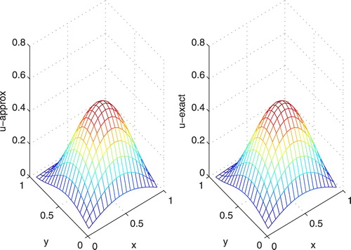The exact solution of this problem is $u(x,y)=x\sin \left(\pi y\right)(1+\cos (\pi x\left)\right).$ We applied our methods $T_1$ and $T_2$ to solve this problem. The computed solutions are compared with exact solutions at grid points and the maximum absolute errors of solutions are tabulated in Table 1. The graphs of the exact and computed solutions are given in Figure 1.

Figure 1. Comparison of exact and approximate solutions for Example 6.1 with $(h,k)=(1/20,1/20)$.

Example 6.2

Consider the equation (41) $\begin{array}{rl}\frac{{\mathrm{\partial }}^{2}u}{\mathrm{\partial }{x}^2}+\frac{{\mathrm{\partial }}^{2}u}{\mathrm{\partial }{y}^2}& =2u+6e^{x+y}(2x{y}^2+2x^{2}y-4xy),\\ & 0<x,y<1,\end{array}$(41) subjected to Dirichlet boundary condition u=0 in boundaries of unit square. The exact solution is $u(x,y)=3e^{x+y}(x^2-x)(y^2-y).$ We applied method $T_2$ to solve this problem. The maximum absolute errors and orders of convergence are tabulated in Table 2 and are compared with the results in reference [13].

Example 6.3

Consider the equation (42) $\begin{array}{rl}\frac{{\mathrm{\partial }}^{2}u}{\mathrm{\partial }{x}^2}+\frac{{\mathrm{\partial }}^{2}u}{\mathrm{\partial }{y}^2}& =c^2{\pi }^{2}u-3c^2{\pi }^2\sin \left(c\pi x\right)\sin \left(c\pi y\right),\\ & 0<x,y<1,\end{array}$(42) subjected to Dirichlet boundary condition u=0 in boundaries of unit square. The exact solution is $u(x,y)=\sin \left(c\pi x\right)\sin \left(c\pi y\right).$ We have solved this problem with methods $T_1$ and $T_2$ for two values of c. The maximum absolute errors and orders of convergence of methods are tabulated in Table 3.

7. Conclusion

We applied non-polynomial tension spline approximation in both space directions for the solution of second-order elliptic partial differential equations. Using the parameters adopted in cubic tension spline, we have obtained a scheme of order $O(h^2+k^2)$. Also by appropriate choices of the parameters we have increased the order of accuracy to new scheme of order $O(h^4+k^4)$. The results of the numerical examples show that our methods are accurate and easy applicable.

Disclosure statement

No potential conflict of interest was reported by the authors.

ORCID

Jalil Rashidinia  http://orcid.org/0000-0002-9177-900X

References

- Barkeshli K. Advanced electromagnetics and scattering theory. New York: Springer; 2015.
- Datta S. Quantum transport: atom to transistor. London: Cambridge University Press; 2005.
- Borden B. Radar imaging of airborne targets. New York: Taylor & Francis; 1999.
- Tian Z. An high order compact finite difference scheme for the second dimensional Poisson equation. J Northwest Univ. 1996;26(2):109–114.
- Zhang J. Multigrid method and fourth order compact scheme for 2d Poisson equation with unequal meshsize discretization. J Comput Phys. 2002;179:170–179. doi: 10.1006/jcph.2002.7049
- Zapata RIMU. High-order implicit finite difference schemes for the two-dimensional Poisson equation. Appl Math Comput. 2017;309:222–244.
- Wang Y, Zhang J. Sixth order compact scheme combined with multigrid method and extrapolation technique for 2d Poisson equation. J Comput Phys. 2009;228:137–146. doi: 10.1016/j.jcp.2008.09.002
- Singer I, Turkel E. High-order finite difference methods for the Helmholtz equation. Comput Method Appl Math. 1998;163:343–358.
- Fu Y. Compact fourth order finite difference schemes for Helmholtz equation with high wave numbers. J Comput Math. 2008;26:98–111.
- Romenski V. The method of spline collocation for the Poisson equation. J Comput Acoust. 1979;81:81–86.
- Bialecki B. Superconvergence of orthogonal spline collocation in the solution of Poisson's equation. Numer Methods Partial Diff Eqn. 1999;15:285–303. doi: 10.1002/(SICI)1098-2426(199905)15:3<285::AID-NUM2>3.0.CO;2-1
- Christara CC. Quadratic spline collocation methods for elliptic partial differential equations. BIT. 1994;34:33–61. doi: 10.1007/BF01935015
- Houstis E, Vavalis E, Rice J. Convergence of o(h4) cubic spline collocation methods for elliptic partial differential equations. SIAM J Numer Anal. 1988;25(1):54–74. doi: 10.1137/0725006
- Fairweather G, Karageorghis A, Maack J. Compact optimal quadratic spline collocation methods for the Helm-holtz equation. J Comput Phys. 2011;230:2880–2895. doi: 10.1016/j.jcp.2010.12.041
- Rashidinia J, Mohammadi R, Ghasemi M. Cubic spline solution of singularly perturbed boundary value problems with significant first derivatives. Appl Math Comput. 2007;190:1762–1766.
- Rashidinia J, Mohammadi R, Jalilian R. Spline solution of nonlinear singular boundary value problems. Int J Comput Math. 2008;85:39–52. doi:10.1080/00207160701293048
- Khan I, Aziz T. Tension spline method for second-order singularly perturbed boundary-value problems. Int J Comput Math. 2005;82(12):1547–1553. doi:10.1080/00207160410001684280
- Aghamohamadi M, Rashidinia J, Ezzati R. Tension spline method for solution of non-linear Fisher equation. Appl Math Comput. 2014;249:399–407.
- Rashidinia J, Mohammadi R. Tension spline solution of nonlinear sine-Gordon equation. Numer Algor. 2011;56:129–142. doi:10.1007/s11075-010-9377-x
- Mohanty R, Dey S. A new finite difference discretization of order four for (∂u/∂n) for two dimensional quasi-linear elliptic boundary value problems. Int J Comput Math. 2001;76:505–516. doi: 10.1080/00207160108805043
- Mohanty R, Jain MK, Dhall D. High accuracy cubic spline approximation for two dimensional quassi-linear elliptic boundary value problems. Int J Comput Math. 2013;37:155–171.
- Yaw K, Kossi E. Higher-order accurate finite volume discretization of Helmholtz equations with pollution effects reductions. Int J Innov Edu Res. 2018;6(2):130–148.
- Ghimire BK, Tian HY, Lamichhane A. Numerical solutions of elliptic partial differential equations using Chebyshev polynomials. Comput Math Appl. 2016;72:1042–1054. doi: 10.1016/j.camwa.2016.06.012
- Dangal T, Chena C, Lin J. Polynomial particular solutions for solving elliptic partial differential equations. Comput Math Appl. 2017;73:60–70. doi: 10.1016/j.camwa.2016.10.024
- Shiralashetti S, Kantli M, Deshi AB. A new wavelet multigrid method for the numerical solution of elliptic type differential equations. Alex Eng J. 2018;57(1):203–209. doi:10.1016/j.aej.2016.12.007