A projection method for linear Fredholm–Volterra integro-differential equations

ABSTRACT

In this study, a collocation method, one of the type of projection methods based on the generalized Bernstein polynomials, is developed for the solution of high-order linear Fredholm–Volterra integro-differential equations containing derivatives of unknown function in the integral part. The method is valid for the mixed conditions. The convergence analysis and error bounds of the method are also given. Besides, six examples are presented to demonstrate the applicability and validity of the method.

KEYWORDS:

• Bernstein polynomials
• polynomial approach
• collocation method
• linear Fredholm–Volterra integro-differential equations

AMS Subject Classifications:

• 45J05
• 65L60

1. Introduction

In the early 1900s, Vito Volterra has introduced new type of equations called as integro-differential equations for his research study on population growth phenomenon. It is clear that one or more derivatives of the unknown function appear out under the integral sign in this type of equations. Many physical and mathematical problems, such as chemical, biological, mechanical, engineering, financial, industrial and so on, can be modelled by integro-differential equations. The applications of integro-differential equations are also important in electromagnetism physics and fluid dynamics. Scientists and engineers come across with the integro-differential equations in their research work including transfers of the heat and mass, problems of the electrical circuit and biological diversity. Since it is not usually possible to find an exact solution of the integro-differential equations, new trends on the numerical methods for solving these types of equations have been developed with calculating techniques and programming supports. One of the most frequently used numerical method is collocation method. In recent years, collocation methods such as Bessel [1], Chebyshev [2,3], Taylor polynomials [4] and B-spline functions [5] have been given for approximating the solutions of linear Fredholm–Volterra integro-differential equations.

In this paper, by benefiting from the definition of the generalized Bernstein polynomials and their approach [6] we develop a collocation method for approximating the solution of $m\mathrm{t}\mathrm{h}$-order linear Fredholm–Volterra integro-differential equation in the most general form as (1) $\begin{array}{rl}\sum _{k=0}^m{a}_k\left(x\right)y^{\left(k\right)}\left(x\right)& =g\left(x\right)+{\lambda }_1{\int }_a^b\sum _{k=0}^q{f}_k\left(x,t\right)y^{\left(k\right)}\left(t\right)\mathrm{d}t\\ & +{\lambda }_2{\int }_a^x\sum _{k=0}^r{v}_k\left(x,t\right)y^{\left(k\right)}\left(t\right)\mathrm{d}t\end{array}$(1) under the mixed conditions (2) $\begin{array}{rl}\sum _{k=0}^{m-1}\sum _{j=0}^l{\tau }_{ij}^k{y}^{\left(k\right)}\left(c_j\right)& ={\mu }_i;i=0,1,\dots ,m-1,\\ & a\le c_j\le b\end{array}$(2) where $a_k\left(x\right)$, $g\left(x\right)$, $f_k(x,t)$ and $v_k(x,t)$ are defined functions respectively on the interval $[a,b]$ and $[a,b]\times [a,b]$, $y\left(x\right)$ is an unknown function, ${\tau }_{ij}^k$, $c_j$, ${\mu }_i$, ${\lambda }_1$ and ${\lambda }_2$ are known constants and $m\ge q,r$. To solve approximately integro-differential equation (1(1) $\begin{array}{rl}\sum _{k=0}^m{a}_k\left(x\right)y^{\left(k\right)}\left(x\right)& =g\left(x\right)+{\lambda }_1{\int }_a^b\sum _{k=0}^q{f}_k\left(x,t\right)y^{\left(k\right)}\left(t\right)\mathrm{d}t\\ & +{\lambda }_2{\int }_a^x\sum _{k=0}^r{v}_k\left(x,t\right)y^{\left(k\right)}\left(t\right)\mathrm{d}t\end{array}$(1) ), we should select a solution that satisfy the equation approximately. In other words, the solution should be close to the exact solution of Equation 1(1) $\begin{array}{rl}\sum _{k=0}^m{a}_k\left(x\right)y^{\left(k\right)}\left(x\right)& =g\left(x\right)+{\lambda }_1{\int }_a^b\sum _{k=0}^q{f}_k\left(x,t\right)y^{\left(k\right)}\left(t\right)\mathrm{d}t\\ & +{\lambda }_2{\int }_a^x\sum _{k=0}^r{v}_k\left(x,t\right)y^{\left(k\right)}\left(t\right)\mathrm{d}t\end{array}$(1) . There are various methods to get the approximate solution. The most popular of these is the collocation method. Moreover, this method can be called as projection method because the collocation method makes essential use of projection (linear) operators [7].

Let's give the following Theorem 1.1 (see [8]) that is an important relation between the generalized Bernstein basis polynomials and their derivatives.

Theorem 1.1

The derivatives of the generalized Bernstein basis polynomials hold the following relation: ${\mathbf{P}}^{\left(k\right)}\left(x\right)\mathbf{=}\mathbf{P}\left(x\right){\mathbf{N}}^k;k=0,1,\dots ,m.$ Here $\mathbf{P}\left(x\right)=\left[\begin{array}{c}{\mathit{p}}_{i,n}\left(x\right)\end{array}\right]$, ${\mathbf{P}}^k\left(x\right)=\left[\begin{array}{c}{\mathit{p}}_{i,n}^{\left(k\right)}\left(x\right)\end{array}\right]$ are $1\times (n+1)$ matrices, $\mathbf{N}\mathbf{=}\left(d_{ij}\right)$ is $(n+1)\times (n+1)$ matrix such that the elements of $\mathbf{N}$ are defined by $d_{ij}=\frac{1}{b-a}\left\{\begin{array}{ll}n-i;& \mathrm{i}\mathrm{f}j=i+1\\ 2i-n;& \mathrm{i}\mathrm{f}j=i\\ -i;& \mathrm{i}\mathrm{f}j=i-1\\ 0;& \mathrm{o}\mathrm{t}\mathrm{h}\mathrm{e}\mathrm{r}\mathrm{w}\mathrm{i}\mathrm{s}\mathrm{e}\end{array}\right.$ for $i,j=0,1,\dots ,n$ and ${\mathbf{N}}^0=\mathbf{I}$ is identity matrix. Here ${\mathit{p}}_{i,n}\left(x\right)$ are generalized Bernstein basis polynomials defined on $[a,b]$.

In the reminder of this paper, the collocation method for linear integro-differential equations is presented, and then convergence and error bounds of the method are analysed. After that, some numerical examples are also given to demonstrate the efficiency of the method.

2. Method of solution

Theorem 2.1

Let $x_s$ be collocation points and $y\in \mathbb{C}[a,b]$. By means of the generalized Bernstein polynomials, the linear Fredholm–Volterra integro-differential equation (1(1) $\begin{array}{rl}\sum _{k=0}^m{a}_k\left(x\right)y^{\left(k\right)}\left(x\right)& =g\left(x\right)+{\lambda }_1{\int }_a^b\sum _{k=0}^q{f}_k\left(x,t\right)y^{\left(k\right)}\left(t\right)\mathrm{d}t\\ & +{\lambda }_2{\int }_a^x\sum _{k=0}^r{v}_k\left(x,t\right)y^{\left(k\right)}\left(t\right)\mathrm{d}t\end{array}$(1) ) can be reduced to the following matrix equation: (3) $\left[\sum _{k=0}^m{\mathbf{A}}_k{\mathbf{P}\mathbf{N}}^k\mathbf{-}{\lambda }_1\sum _{k=0}^q{\mathbf{F}}_k{\mathbf{N}}^k\mathbf{-}{\lambda }_2\sum _{k=0}^r{\mathbf{V}}_k{\mathbf{N}}^k\right]\mathbf{Y}=\mathbf{G}\mathbf{.}$(3) Here ${\mathbf{A}}_k=diag\left[{\mathit{a}}_k\right(x_s\left)\right],$ ${\mathbf{F}}_j\mathbf{=}\left[{\mathit{F}}_{k,s,i}\right],$ $\mathbf{V}\mathbf{=}\left[{\mathit{V}}_{k,s,i}\right],$ $\mathbf{P}=\left[{\mathit{p}}_{i,n}\right(x_s\left)\right]$ are $(n+1)\times (n+1)$ matrices, and $\mathbf{Y}\mathbf{=}\left[\mathit{y}\right(a+(b-a)i/n\left)\right],$ $\mathbf{G}\mathbf{=}\left[g\right(x_s\left)\right]$ are $(n+1)\times 1$ matrices for $i,s=0,1,\dots ,n$. Besides, the elements of $\mathbf{F}$ and $\mathbf{V}$ matrices are defined as $\begin{array}{rl}{\mathit{F}}_{k,s,i}& ={\int }_a^b{f}_k\left(x_s,t\right)p_{i,n}\left(t\right)\mathrm{d}t,\\ {\mathit{V}}_{k,s,i}& ={\int }_a^{x_s}{v}_k\left(x_s,t\right)p_{i,n}\left(t\right)\mathrm{d}t.\end{array}$

Proof.

Since $y\left(x\right)$ $\in \mathbb{C}[a,b]$, Equation 1(1) $\begin{array}{rl}\sum _{k=0}^m{a}_k\left(x\right)y^{\left(k\right)}\left(x\right)& =g\left(x\right)+{\lambda }_1{\int }_a^b\sum _{k=0}^q{f}_k\left(x,t\right)y^{\left(k\right)}\left(t\right)\mathrm{d}t\\ & +{\lambda }_2{\int }_a^x\sum _{k=0}^r{v}_k\left(x,t\right)y^{\left(k\right)}\left(t\right)\mathrm{d}t\end{array}$(1) has the generalized Bernstein polynomial solution, therefore the following is satisfied: $y\left(x\right)\cong B_n(y;x)=\sum _{i=0}^{n}y\left(a+\frac{(b-a)i}{n}\right)p_{i,n}\left(x\right),$ (4) $y\left(x\right)\cong \mathbf{P}\left(x\right)\mathbf{Y}$(4) such that $\begin{array}{rl}\mathbf{Y}& =\left[\mathit{y}\left(a\right)\mathit{y}\left(a+\frac{b-a}{n}\right)\dots \right.\\ & {\left.\mathit{y}\left(a+\frac{\left(b-a\right)\left(n-1\right)}{n}\right)\mathit{y}\left(b\right)\right]}^T.\end{array}$ Using Theorem 1.1, expression (4(4) $y\left(x\right)\cong \mathbf{P}\left(x\right)\mathbf{Y}$(4) ) can be rewritten as (5) $y^{\left(k\right)}\left(x\right)\simeq {\mathbf{P}}^{\left(k\right)}\left(x\right)\mathbf{Y}\mathbf{=}\mathbf{P}\left(x\right){\mathbf{N}}^k\mathbf{Y};k=0,1,\dots ,m.$(5) By substituting relation (5(5) $y^{\left(k\right)}\left(x\right)\simeq {\mathbf{P}}^{\left(k\right)}\left(x\right)\mathbf{Y}\mathbf{=}\mathbf{P}\left(x\right){\mathbf{N}}^k\mathbf{Y};k=0,1,\dots ,m.$(5) ) and the collocation points into integro-differential equation (1(1) $\begin{array}{rl}\sum _{k=0}^m{a}_k\left(x\right)y^{\left(k\right)}\left(x\right)& =g\left(x\right)+{\lambda }_1{\int }_a^b\sum _{k=0}^q{f}_k\left(x,t\right)y^{\left(k\right)}\left(t\right)\mathrm{d}t\\ & +{\lambda }_2{\int }_a^x\sum _{k=0}^r{v}_k\left(x,t\right)y^{\left(k\right)}\left(t\right)\mathrm{d}t\end{array}$(1) ), linear algebraic equation system is obtained in the form: (6) $\begin{array}{rl}& \sum _{k=0}^m{a}_k\left(x_s\right)\mathbf{P}\left(x_s\right){\mathbf{N}}^k\mathbf{Y}\\ & =g\left(x_s\right)+{\lambda }_1{\int }_a^b\sum _{k=0}^q{f}_k\left(x_s,t\right)\mathbf{P}\left(t\right){\mathbf{N}}^k\mathbf{Y}\mathrm{d}t\\ & +{\lambda }_2{\int }_a^{x_s}\sum _{k=0}^r{v}_k\left(x_s,t\right)\mathbf{P}\left(t\right){\mathbf{N}}^k\mathbf{Y}\mathrm{d}t.\end{array}$(6) Here, it is obvious that $y^{\left(k\right)}\left(x_s\right)=B_n^{\left(k\right)}(y;x_s)$ $(s=0,1,\dots ,n)$ from the definition of the collocation method. This system can also be written in the compact form as (7) $\begin{array}{rl}& \left[\sum _{k=0}^m{a}_k\left(x_s\right)\mathbf{P}\left(x_s\right){\mathbf{N}}^k-{\lambda }_1\sum _{k=0}^q{\mathbf{F}}_k\left(x_s\right){\mathbf{N}}^k\right.\\ & -\left.{\lambda }_2\sum _{k=0}^r{\mathbf{V}}_k\left(x_s\right){\mathbf{N}}^k\right]\mathbf{Y}=g\left(x_s\right)\end{array}$(7) such that $\begin{array}{rl}{\mathbf{F}}_k\left(x_s\right)& ={\int }_a^b{f}_k\left(x_s,t\right)\mathbf{P}\left(t\right)\mathrm{d}t,\\ {\mathbf{V}}_k\left(x_s\right)& ={\int }_a^{x_s}{v}_k\left(x_s,t\right)\mathbf{P}\left(t\right)\mathrm{d}t.\end{array}$ Therefore, Equation 7(7) $\begin{array}{rl}& \left[\sum _{k=0}^m{a}_k\left(x_s\right)\mathbf{P}\left(x_s\right){\mathbf{N}}^k-{\lambda }_1\sum _{k=0}^q{\mathbf{F}}_k\left(x_s\right){\mathbf{N}}^k\right.\\ & -\left.{\lambda }_2\sum _{k=0}^r{\mathbf{V}}_k\left(x_s\right){\mathbf{N}}^k\right]\mathbf{Y}=g\left(x_s\right)\end{array}$(7) for $s=0,1,\dots ,n$ can be written in the desired matrix form (3(3) $\left[\sum _{k=0}^m{\mathbf{A}}_k{\mathbf{P}\mathbf{N}}^k\mathbf{-}{\lambda }_1\sum _{k=0}^q{\mathbf{F}}_k{\mathbf{N}}^k\mathbf{-}{\lambda }_2\sum _{k=0}^r{\mathbf{V}}_k{\mathbf{N}}^k\right]\mathbf{Y}=\mathbf{G}\mathbf{.}$(3) ) and the proof is completed.

The matrices in Equation 3(3) $\left[\sum _{k=0}^m{\mathbf{A}}_k{\mathbf{P}\mathbf{N}}^k\mathbf{-}{\lambda }_1\sum _{k=0}^q{\mathbf{F}}_k{\mathbf{N}}^k\mathbf{-}{\lambda }_2\sum _{k=0}^r{\mathbf{V}}_k{\mathbf{N}}^k\right]\mathbf{Y}=\mathbf{G}\mathbf{.}$(3) are obviously denoted by $\begin{array}{rl}{\mathbf{A}}_k& =\left[\begin{array}{cccc}{\mathit{a}}_k\left(x_0\right)& 0& \dots & 0\\ 0& {\mathit{a}}_k\left(x_1\right)& \dots & 0\\ ⋮& ⋮& \ddots & ⋮\\ 0& 0& \dots & {\mathit{a}}_k\left(x_n\right)\end{array}\right],\mathbf{G}=\left[\begin{array}{c}\mathit{g}\left(x_0\right)\\ \mathit{g}\left(x_1\right)\\ ⋮\\ \mathit{g}\left(x_n\right)\end{array}\right],\\ \mathbf{P}& =\left[\begin{array}{c}\mathbf{P}\left(x_0\right)\\ \mathbf{P}\left(x_1\right)\\ ⋮\\ \mathbf{P}\left(x_n\right)\end{array}\right],{\mathbf{F}}_k=\left[\begin{array}{c}{\mathbf{F}}_k\left(x_0\right)\\ {\mathbf{F}}_k\left(x_1\right)\\ ⋮\\ {\mathbf{F}}_k\left(x_n\right)\end{array}\right],{\mathbf{V}}_k=\left[\begin{array}{c}{\mathbf{V}}_k\left(x_0\right)\\ {\mathbf{V}}_k\left(x_1\right)\\ ⋮\\ {\mathbf{V}}_k\left(x_n\right)\end{array}\right].\end{array}$ General linear integro-differential equation (1(1) $\begin{array}{rl}\sum _{k=0}^m{a}_k\left(x\right)y^{\left(k\right)}\left(x\right)& =g\left(x\right)+{\lambda }_1{\int }_a^b\sum _{k=0}^q{f}_k\left(x,t\right)y^{\left(k\right)}\left(t\right)\mathrm{d}t\\ & +{\lambda }_2{\int }_a^x\sum _{k=0}^r{v}_k\left(x,t\right)y^{\left(k\right)}\left(t\right)\mathrm{d}t\end{array}$(1) ) under mixed conditions (2(2) $\begin{array}{rl}\sum _{k=0}^{m-1}\sum _{j=0}^l{\tau }_{ij}^k{y}^{\left(k\right)}\left(c_j\right)& ={\mu }_i;i=0,1,\dots ,m-1,\\ & a\le c_j\le b\end{array}$(2) ) can be solved by the following steps:

Step 1. Equation 3(3) $\left[\sum _{k=0}^m{\mathbf{A}}_k{\mathbf{P}\mathbf{N}}^k\mathbf{-}{\lambda }_1\sum _{k=0}^q{\mathbf{F}}_k{\mathbf{N}}^k\mathbf{-}{\lambda }_2\sum _{k=0}^r{\mathbf{V}}_k{\mathbf{N}}^k\right]\mathbf{Y}=\mathbf{G}\mathbf{.}$(3) can be written simply as follows: (8) $\mathbf{W}\mathbf{Y}\mathbf{=}\mathbf{G}\mathrm{o}\mathrm{r}\left[\mathbf{W}\mathbf{;}\mathbf{G}\right]$(8) so that $\mathbf{W}\mathbf{=}\sum _{k=0}^m{\mathbf{A}}_k{\mathbf{P}\mathbf{N}}^k\mathbf{-}{\lambda }_1\sum _{k=0}^q{\mathbf{F}}_k{\mathbf{N}}^k\mathbf{-}{\lambda }_2\sum _{k=0}^r{\mathbf{V}}_k{\mathbf{N}}^k$. Here $\mathbf{Y}$ is n+1-dimensional unknown matrix. The matrix equation corresponds to a linear algebraic system. First, $\mathbf{W}$ and $\mathbf{G}$ are calculated.

Step 2. From expression (5(5) $y^{\left(k\right)}\left(x\right)\simeq {\mathbf{P}}^{\left(k\right)}\left(x\right)\mathbf{Y}\mathbf{=}\mathbf{P}\left(x\right){\mathbf{N}}^k\mathbf{Y};k=0,1,\dots ,m.$(5) ), the matrix form of mixed conditions (2(2) $\begin{array}{rl}\sum _{k=0}^{m-1}\sum _{j=0}^l{\tau }_{ij}^k{y}^{\left(k\right)}\left(c_j\right)& ={\mu }_i;i=0,1,\dots ,m-1,\\ & a\le c_j\le b\end{array}$(2) ) can be written as (9) ${\mathbf{U}}_i\mathbf{Y}={\mu }_i\mathrm{o}\mathrm{r}\left[{\mathbf{U}}_i;{\mu }_i\right];i=0,\dots ,m-1.$(9) Here $\mathbf{U}$ is evaluated by ${\mathbf{U}}_i=\sum _{k=0}^{m-1}\sum _{j=0}^l{\tau }_{ij}^k\mathbf{P}\left(c_j\right){\mathbf{N}}^k$.

Step 3. Let $[\tilde{\mathbf{W}};\tilde{\mathbf{G}}]$ be denoted as new augmented matrix that is acquired by adding the elements of augmented row matrices (9(9) ${\mathbf{U}}_i\mathbf{Y}={\mu }_i\mathrm{o}\mathrm{r}\left[{\mathbf{U}}_i;{\mu }_i\right];i=0,\dots ,m-1.$(9) ) to the end of augmented matrix (8(8) $\mathbf{W}\mathbf{Y}\mathbf{=}\mathbf{G}\mathrm{o}\mathrm{r}\left[\mathbf{W}\mathbf{;}\mathbf{G}\right]$(8) ). If the number of collocation points is S=n+1, then $\left[\tilde{\mathbf{W}};\tilde{\mathbf{G}}\right]=\left[\begin{array}{cccccc}{\mathit{w}}_{0,0}& {\mathit{w}}_{0,1}& \dots & {\mathit{w}}_{0,n}& ;& \mathit{g}\left(x_0\right)\\ \dots & \dots & \dots & \dots & ;& \dots \\ {\mathit{w}}_{n,0}& {\mathit{w}}_{n,1}& \dots & {\mathit{w}}_{n,n}& ;& \mathit{g}\left(x_n\right)\\ {\mathit{t}}_{0,0}& {\mathit{t}}_{0,1}& \dots & {\mathit{t}}_{0,n}& ;& {\mu }_0\\ \dots & \dots & \dots & \dots & ;& \dots \\ {\mathit{t}}_{m-1,0}& {\mathit{t}}_{m-1,1}& \dots & {\mathit{t}}_{m-1,n}& ;& {\mu }_{m-1}\end{array}\right],$ such that $\tilde{\mathbf{W}}$ is $(n+m+1)\times (n+1)$ and $\tilde{\mathbf{G}}$ is $(n+m+1)\times 1$ dimensional matrices. Besides the augmented matrix can be defined as $[{\mathbf{W}}^{\ast };{\mathbf{G}}^{\ast }]$ that is obtained by replacing the m rows of augmented matrix (8) with the rows of augmented matrix (9) as follows: $\begin{array}{rl}& \left[{\mathbf{W}}^{\ast };{\mathbf{G}}^{\ast }\right]\\ & =\left[\begin{array}{cccccc}{\mathit{w}}_{0,0}& {\mathit{w}}_{0,1}& \dots & {\mathit{w}}_{0,n}& ;& \mathit{g}\left(x_0\right)\\ \dots & \dots & \dots & \dots & ;& \dots \\ {\mathit{t}}_{0,0}& {\mathit{t}}_{0,1}& \dots & {\mathit{t}}_{0,n}& ;& {\mu }_0\\ \dots & \dots & \dots & \dots & ;& \dots \\ {\mathit{t}}_{m-1,0}& {\mathit{t}}_{m-1,1}& \dots & {\mathit{t}}_{m-1,n}& ;& {\mu }_{m-1}\\ \dots & \dots & \dots & \dots & \dots & \dots \\ {\mathit{w}}_{n-m,0}& {\mathit{w}}_{n-m,1}& \dots & {\mathit{w}}_{n-m,0}& ;& \mathit{g}\left(x_n\right)\end{array}\right].\end{array}$ In this case, ${\mathbf{W}}^{\ast }$ is $(n+1)\times (n+1)$ and ${\mathbf{G}}^{\ast }$ is $(n+1)\times 1$ dimensional matrices.

Step 4. When $rank\left({\mathbf{W}}^{\ast }\right)=rank[{\mathbf{W}}^{\ast };{\mathbf{G}}^{\ast }]=n+1$ or $rank\left(\tilde{\mathbf{W}}\right)=rank[\tilde{\mathbf{W}};\tilde{\mathbf{G}}]=n+1$, the unknown coefficient matrix $\mathbf{Y}$ is uniquely determined [9]. Then, this system can be solved by the Gauss Elimination, Generalized Inverse, LU and QR factorization methods.

3. Convergence and error analysis

Definition 3.1

The maximum error can be defined as ${∥e_n∥}_{\mathrm{\infty }}=\underset{a\le x\le b}{max}\left|y\left(x\right)-y_n\left(x\right)\right|$ where $y\left(x\right)$ and $y_n\left(x\right)$ are exact and approximate solutions, respectively. Impending $f\in \mathbb{C}$ $[a,b]\times \mathbb{C}[a,b]$, the maximum norm can be denoted by ${∥f∥}_{\mathrm{\infty }}=\underset{x,t\in \left[a,b\right]}{max}\left|f\left(x,t\right)\right|.$ Besides maximum, mean and root of the mean square errors at the collocation points can be calculated respectively by the following formulas: $\begin{array}{rl}{E}_{max}& =\underset{x_s\in \left[a,b\right]}{max}\left|e_n\left(x_s\right)\right|,E_{\mathrm{m}\mathrm{e}\mathrm{a}\mathrm{n}}=\frac{1}{n+1}\sum _{s=0}^n\left|e_n\left(x_s\right)\right|,\\ E_{\mathrm{r}\mathrm{o}\mathrm{o}\mathrm{t}}& =\sqrt{\frac{1}{n+1}\sum _{s=0}^n(e_n\left(x_s\right){)}^2}.\end{array}$ In addition, residual error for the confessed Bernstein collocation method can be expressed as (10) $\begin{array}{rl}{R}_n\left(x\right)& =\sum _{k=0}^m{a}_k\left(x\right)B_n^{\left(k\right)}(y;x)\\ & -{\lambda }_1{\int }_a^b\sum _{k=0}^q{f}_k\left(x,t\right)B_n^{\left(k\right)}(y;t)\mathrm{d}t\\ & -{\lambda }_2{\int }_a^x\sum _{k=0}^r{v}_k\left(x,t\right)B_n^{\left(k\right)}(y;t)\mathrm{d}t-g\left(x\right).\end{array}$(10)

Theorem 3.1

If $y\in {\mathbb{C}}^{k+2}[a,b],$ then the following inequality is hold for some $k\ge 0:$ $\begin{array}{rl}& \left|B_n^{\left(k\right)}\left(y;x\right)-y^{\left(k\right)}\left(x\right)\right|\le \frac{1}{2n}\left(k\left(k-1\right){∥y^{\left(k\right)}∥}_{\mathrm{\infty }}+k\left|b\right.\right.\\ & +a-\left.2x\right|\left.{∥y^{\left(k+1\right)}∥}_{\mathrm{\infty }}+\left(x-a\right)\left(b-x\right){∥y^{\left(k+2\right)}∥}_{\mathrm{\infty }}\right).\end{array}$

Proof.

The above theorem can be easily proved by considering the induction technique and transformation $t=(x-a)/(b-a)$ like the theorem presented on the interval $[0,1]$ by DeVore and Lorentz [10].

Considering k=0 and the definition of the maximum norm in the Theorem 3.1, the following corollary can be noted:

Corollary 3.1

If $y\in {\mathbb{C}}^2[a,b],$ then the following inequality is hold: $\left|B_n\left(y;x\right)-y\left(x\right)\right|\le \frac{{\left(b-a\right)}^2}{8n}{∥y^{\mathrm{\prime }\mathrm{\prime }}∥}_{\mathrm{\infty }}.$

Theorem 3.2

Let $x_s\in [a,b]$ be collocation points. If f, $v\in \mathbb{C}[a,b]\times \mathbb{C}[a,b]$ and $a_k,$ $y^{\left(k\right)}\in \mathbb{C}[a,b]$ for $k=0,1,\dots ,m+2,$ then the residual errors hold the following inequality at the collocation points: $\left|R_n\left(x_s\right)\right|\le \frac{1}{2n}\left[\left|{\lambda }_1\right|\left(b-a\right)\sigma \left(x_s\right)+\left|{\lambda }_2\right|\left(x_s-a\right)\tau \left(x_s\right)\right]$ and $\underset{n\to \mathrm{\infty }}{lim}\left|R_n\right(x_s\left)\right|=0$. Here σ and τ are constants which depend on the collocation points.

Proof.

By taking $g\left(x\right)$ from Equation 1(1) $\begin{array}{rl}\sum _{k=0}^m{a}_k\left(x\right)y^{\left(k\right)}\left(x\right)& =g\left(x\right)+{\lambda }_1{\int }_a^b\sum _{k=0}^q{f}_k\left(x,t\right)y^{\left(k\right)}\left(t\right)\mathrm{d}t\\ & +{\lambda }_2{\int }_a^x\sum _{k=0}^r{v}_k\left(x,t\right)y^{\left(k\right)}\left(t\right)\mathrm{d}t\end{array}$(1) and substituting it in residual error (10(10) $\begin{array}{rl}{R}_n\left(x\right)& =\sum _{k=0}^m{a}_k\left(x\right)B_n^{\left(k\right)}(y;x)\\ & -{\lambda }_1{\int }_a^b\sum _{k=0}^q{f}_k\left(x,t\right)B_n^{\left(k\right)}(y;t)\mathrm{d}t\\ & -{\lambda }_2{\int }_a^x\sum _{k=0}^r{v}_k\left(x,t\right)B_n^{\left(k\right)}(y;t)\mathrm{d}t-g\left(x\right).\end{array}$(10) ), the absolute residual error can be written as follows: (11) $\begin{array}{rl}\left|R_n\left(x\right)\right|& \le \sum _{k=0}^m\left|a_k\left(x\right)\right|\left|B_n^{\left(k\right)}(y;x)-y^{\left(k\right)}\left(x\right)\right|\\ & +\left|{\lambda }_1\right|{\int }_a^b\sum _{k=0}^q\left|f_k\left(x,t\right)\right|\left|B_n^{\left(k\right)}(y;t)-y^{\left(k\right)}\left(t\right)\right|\mathrm{d}t\\ & +\left|{\lambda }_2\right|{\int }_a^x\sum _{k=0}^r\left|v_k(x,t)\right|\left|B_n^{\left(k\right)}(y;t)-y^{\left(k\right)}\left(t\right)\right|\mathrm{d}t.\end{array}$(11) Since $y^{\left(k\right)}\in \mathbb{C}[a,b]$ and $B_n^{\left(k\right)}(y;x_s)=y^{\left(k\right)}\left(x_s\right)$ for $s=0,1,\dots ,n$ and $k=0,1,\dots ,m+2$, the residual errors provide the following inequality: $\begin{array}{rl}\left|R_n\left(x_s\right)\right|\le & \left|{\lambda }_1\right|{\int }_a^b\sum _{k=0}^q\left|f_k\left(x_s,t\right)\right|\left|B_n^{\left(k\right)}(y;t)-y^{\left(k\right)}\left(t\right)\right|\mathrm{d}t\\ & +\left|{\lambda }_2\right|{\int }_a^{x_s}\sum _{k=0}^r\left|v_k(x_s,t)\right|\left|B_n^{\left(k\right)}(y;t)-y^{\left(k\right)}\left(t\right)\right|\mathrm{d}t.\end{array}$ If Theorem 3.1 is applied to the right side of the inequality, then we have $\begin{array}{rl}\left|R_n\left(x_s\right)\right|& \le \frac{1}{2n}\left[\left|{\lambda }_1\right|{\int }_a^b\sum _{k=0}^q\left|f_k\left(x_s,t\right)\right|\left(k\left(k-1\right)∥y^{\left(k\right)}∥\right.\right.\\ & +k\left|b+a-2t\right|∥y^{\left(k+1\right)}∥\\ & +\left.\left(t-a\right)\left(b-t\right)∥y^{\left(k+2\right)}∥\right)\mathrm{d}t\\ & +\left|{\lambda }_2\right|{\int }_a^{x_s}\sum _{k=0}^r\left|v_k\left(x_s,t\right)\right|\left(k\left(k-1\right)∥y^{\left(k\right)}∥\right.\\ & +k\left|b+a-2t\right|∥y^{\left(k+1\right)}∥\\ & +\left.\left.\left(t-a\right)\left(b-t\right)∥y^{\left(k+2\right)}∥\right)\mathrm{d}t\right].\end{array}$ If we take the maximum of the right side of this inequality with regard to t, then we can rewrite the residual error bound as $\begin{array}{rl}\left|R_n\left(x_s\right)\right|& \le \frac{1}{2n}\left[\left|{\lambda }_1\right|\left(b-a\right)\sum _{k=0}^q{\epsilon }_k\left(x_s\right)S_k\right.\\ & +\left.\left|{\lambda }_2\right|\left(x_s-a\right)\sum _{k=0}^r{\rho }_k\left(x_s\right)S_k\right]\end{array}$ such that $\underset{t\in \left[a,b\right]}{max}\left|f_k\left(x_s,t\right)\right|={\epsilon }_k\left(x_s\right),\underset{t\in \left[a,b\right]}{max}\left|v_k\left(x_s,t\right)\right|={\rho }_k\left(x_s\right)$ and $\begin{array}{rl}{S}_k& =k\left(k-1\right)∥y^{\left(k\right)}∥+k\left(b-a\right)∥y^{\left(k+1\right)}∥\\ & +\frac{{\left(b-a\right)}^2}{4}∥y^{\left(k+2\right)}∥.\end{array}$ Denoting $\sigma \left(x_s\right)=\sum _{k=0}^q{\epsilon }_k\left(x_s\right)S_k\mathrm{a}\mathrm{n}\mathrm{d}\tau \left(x_s\right)=\sum _{k=0}^r{\rho }_k\left(x_s\right)S_k,$ we obtain the desired result. Since σ and τ are constants, $\left|R_n\right(x_s\left)\right|\to 0$ as $n\to \mathrm{\infty }$. This completes the proof.

Theorem 3.3

If f, $v\in \mathbb{C}[a,b]\times \mathbb{C}[a,b]$ and $y^{\left(k\right)}\in \mathbb{C}[a,b]$ $(k=0,1,\dots ,m+2),$ then residual error bound has the following inequality: ${∥R_n∥}_{\mathrm{\infty }}\le \frac{1}{2n}\left[\theta +\left(b-a\right)\left(\left|{\lambda }_1\right|\phi +\left|{\lambda }_2\right|\varphi \right)\right]$ and convergency: $\underset{n\to \mathrm{\infty }}{lim}{∥R_n∥}_{\mathrm{\infty }}=0$ such that θ, φ and ϕ are positive constants: $\begin{array}{rl}\theta & =\sum _{k=0}^m{∥a_k∥}_{\mathrm{\infty }}{S}_k,\phi =\sum _{k=0}^q{∥f_k∥}_{\mathrm{\infty }}{S}_k\mathrm{a}\mathrm{n}\mathrm{d}\\ \varphi & =\sum _{k=0}^r{∥v_k∥}_{\mathrm{\infty }}{S}_k\end{array}$ where $S_k$ is denoted as in Theorem 3.2.

Proof.

Applying Theorem 3.1 to the right-hand side of inequality (11(11) $\begin{array}{rl}\left|R_n\left(x\right)\right|& \le \sum _{k=0}^m\left|a_k\left(x\right)\right|\left|B_n^{\left(k\right)}(y;x)-y^{\left(k\right)}\left(x\right)\right|\\ & +\left|{\lambda }_1\right|{\int }_a^b\sum _{k=0}^q\left|f_k\left(x,t\right)\right|\left|B_n^{\left(k\right)}(y;t)-y^{\left(k\right)}\left(t\right)\right|\mathrm{d}t\\ & +\left|{\lambda }_2\right|{\int }_a^x\sum _{k=0}^r\left|v_k(x,t)\right|\left|B_n^{\left(k\right)}(y;t)-y^{\left(k\right)}\left(t\right)\right|\mathrm{d}t.\end{array}$(11) ), we get $\begin{array}{rl}& \left|R_n\right(x\left)\right|\\ & \le \frac{1}{2n}\left[\sum _{k=0}^m\left|a_k\right(x\left)\right|\left(k\right(k-1)\parallel y^{\left(k\right)}\parallel +k|b+a-2x|\right.\\ & \times \parallel y^{(k+1)}\parallel +(x-a)(b-x)\parallel y^{(k+2)}\parallel )\\ & +\left|{\lambda }_1\right|{\int }_a^b\sum _{k=0}^q\left|f_k\right(x,t\left)\right|\left(k\right(k-1)\parallel y^{\left(k\right)}\parallel +k|b+a\\ & -2t|\parallel y^{(k+1)}\parallel +(t-a\left)\right(b-t)\parallel y^{(k+2)}\parallel )\mathrm{d}t\\ & +\left|{\lambda }_2\right|{\int }_a^x\sum _{k=0}^r\left|v_k\right(x,t\left)\right|\left(k\right(k-1)\parallel y^{\left(k\right)}\parallel +k|b+a\\ & -2t|\left.\parallel y^{(k+1)}\parallel +(t-a)(b-t)\parallel y^{(k+2)}\parallel )\mathrm{d}t\right].\end{array}$ From the definition of the maximum error and the properties of the norm, the error bound can be written as $\begin{array}{rl}{∥R_n∥}_{\mathrm{\infty }}& \le \frac{1}{2n}\left[\sum _{k=0}^m{∥a_k∥}_{\mathrm{\infty }}{S}_k+\left|{\lambda }_1\right|{\int }_a^b\sum _{k=0}^q{∥f_k∥}_{\mathrm{\infty }}{S}_k\mathrm{d}t\right.\\ & +\left.\left|{\lambda }_2\right|{\int }_a^x\sum _{k=0}^r{∥v_k∥}_{\mathrm{\infty }}{S}_k\mathrm{d}t\right]\\ & \le \frac{1}{2n}\left[\sum _{k=0}^m{∥a_k∥}_{\mathrm{\infty }}{S}_k+\left|{\lambda }_1\right|\left(b-a\right)\sum _{k=0}^q{∥f_k∥}_{\mathrm{\infty }}{S}_k\right.\\ & +\left.\left|{\lambda }_2\right|\left(b-a\right)\sum _{k=0}^r{∥v_k∥}_{\mathrm{\infty }}{S}_k\right].\end{array}$ If we consider the θ, φ and ϕ as noted above, then the residual error bound is obtained. Since θ, φ and ϕ are constants, $\parallel R_n{\parallel }_{\mathrm{\infty }}\to 0$ as $n\to \mathrm{\infty }$. This completes the proof.

4. Numerical results

The proposed method is tested on six numerical examples. Numerical results of this method are computed in Matlab 7.1 by considering the adding and deleting techniques mentioned in Step 3. Besides, these results and their comparisons with the other methods are demonstrated by the tables and figures.

Example 4.1

Consider the linear Fredholm integro-differential equation with initial conditions as follows: $\begin{array}{rl}{y}^{\left(8\right)}\left(x\right)& =-8e^x+x^2+y\left(x\right)+{\int }_0^1{x}^2{y}^{\mathrm{\prime }}\left(t\right)\mathrm{d}t,\\ y\left(0\right)& =1,y^{\mathrm{\prime }}\left(0\right)=0,y^{\mathrm{\prime }\mathrm{\prime }}\left(0\right)=-1,\\ y^{\mathrm{\prime }\mathrm{\prime }\mathrm{\prime }}\left(0\right)& =-2,y^{\left(4\right)}\left(0\right)=-3,\\ y^{\left(5\right)}\left(0\right)& =-4,y^{\left(6\right)}\left(0\right)=-5,y^{\left(7\right)}\left(0\right)=-6\end{array}$ Exact solution of the above equation is $y\left(x\right)=(1-x)e^x$.

The mean errors that calculated on the collocation points $x_s=s/n$; $s=0,1,\dots ,n$ by the proposed method are indicated with the increasing n values in Table 1. The table exhibited that the numerical solutions attained by deleting the last eight row matrix are better than the numerical solutions attained by adding for increasing n values. However, the absolute errors obtained by adding technique converge faster than the results of the Variational Iteration method [11] given as the iteration k in Table 2. It exhibited that the presented method has more effective numerical results without using iteration than the other method.

Table 1. Mean errors $E_{\mathrm{m}\mathrm{e}\mathrm{a}\mathrm{n}}$ for Example 4.1.

n	$Addingtechnique$	Deleting technique
10	$1.6\mathrm{e}-004$	$9.9\mathrm{e}-009$
11	$2.2\mathrm{e}-007$	$3.5\mathrm{e}-010$
12	$2.1\mathrm{e}-009$	$1.7\mathrm{e}-011$
13	$2.4\mathrm{e}-011$	$2.7\mathrm{e}-012$
14	$1.4\mathrm{e}-012$	$2.5\mathrm{e}-012$

Table 2. Comparison of the $\left|e_n\right(x\left)\right|$ for Example 4.1.

	Presented method	Variational iteration method
x	$n=15,$ k=1	k=10	k=15
0.2	1.6e−012	2.9e−014	1.1e−016
0.4	1.7e−012	3.1e−011	1.2e−014
0.6	1.4e−012	1.9e−009	6.6e−013
0.8	6.3e−013	3.4e−008	1.2e−011
1.0	8.0e−012	3.3e−007	1.1e−010

Example 4.2

Consider the linear Fredholm–Volterra integro-differential equation $\begin{array}{rl}& e^x{y}^{{}^{\mathrm{\prime }\mathrm{\prime }}}\left(x\right)+x^3{y}^{\mathrm{\prime }}\left(x\right)+y\left(x\right)\\ & =-\frac{2}{\pi }\sin \left(\pi x\right)+2e^x+x^2-2x-\frac{1}{3}\\ & +{\int }_{-1}^1\left[\left(x^4-t\right)y\left(t\right)+t^2{y}^{\mathrm{\prime }}\left(t\right)\right]\mathrm{d}t\\ & +{\int }_{-1}^x\left[\cos \left(\pi t\right)y^{\mathrm{\prime }\mathrm{\prime }}\left(t\right)+3tx{y}^{\mathrm{\prime }}\left(t\right)\right]\mathrm{d}t\end{array}$ under the mixed conditions $y(-1)+2y\left(0\right)=0,$ $y^{\mathrm{\prime }}\left(1/2\right)=1,$ $y\left(1\right)=2/3.$ Here the exact solution is $y\left(x\right)=x^2-1/3$.

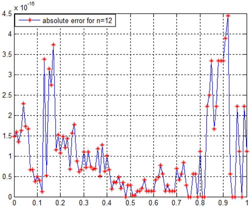
The absolute errors of the method attained by adding and deleting the first and last two row matrices at the collocation points $x_s=\cos \left(s\pi /n\right)$; $s=0,1,\dots ,n$ are given for different n values in Figures 1 and 2. We can see from Figure 1, the best result for n=2 is attained, and note that the exact solution to the problem is a second-degree polynomial.

Figure 1. $\left|e_2\right(x\left)\right|$ for Example 4.2.

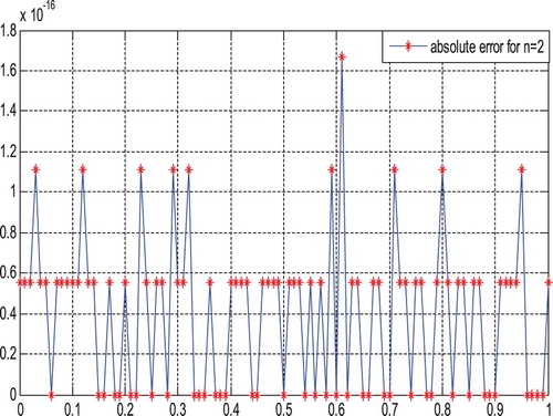
Figure 2. $\left|e_{12}\right(x\left)\right|$ for Example 4.2.

The mean errors at the Chebyshev collocation points $x_s=\cos \left(s\pi /n\right)$; $s=0,1,\dots ,n$ by the presented method are compared with the results by the Chebyshev collocation method [12] in Table 3. The table exhibited that the numerical results attained by adding and deleting both the first and last two row matrices are more effective than the numerical results of the other method.

Table 3. Comparison of the mean errors for Example 4.2.

	Proposed method		Chebyshev collocation
n	Adding technique	Deleting technique	method
2	$5.6\mathrm{e}-017$	$5.6\mathrm{e}-017$	–
3	$8.8\mathrm{e}-017$	$8.8\mathrm{e}-017$	$2.0\mathrm{e}-002$
6	$2.1\mathrm{e}-016$	$1.5\mathrm{e}-016$	$1.2\mathrm{e}-004$
9	$1.8\mathrm{e}-016$	$1.2\mathrm{e}-016$	$1.8\mathrm{e}-006$
12	$2.0\mathrm{e}-016$	$2.1\mathrm{e}-016$	$9.1\mathrm{e}-011$
15	$2.4\mathrm{e}-016$	$3.0\mathrm{e}-015$	$4.2\mathrm{e}-012$

Example 4.3

Let us consider the linear Fredholm–Volterra integro-differential equation $\begin{array}{rl}{y}^{\mathrm{\prime }}\left(x\right)& =\frac{27}{5}-\frac{1}{5}{x}^6-\frac{3}{4}{x}^5-x^4-\frac{1}{2}{x}^3+3x^2\\ & +\frac{41}{20}x+{\int }_{-1}^1\left(x-t\right)y\left(t\right)\mathrm{d}t+{\int }_{-1}^{x}xty\left(t\right)\mathrm{d}t\end{array}$ under the initial condition $y\left(0\right)=1$. Exact solution of the above equation is $y\left(x\right)=(x+1{)}^3$.

We find the exact solution as similar to the Chebyshev collocation method [13] for n=3. If you pay attention, the exact solution of the problem is a third-degree polynomial.

Example 4.4

Consider the Volterra integral equation of the first kind ${\int }_0^x\cos \left(x-t\right)y^{\mathrm{\prime }\mathrm{\prime }}\left(t\right)\mathrm{d}t=2\sin \left(x\right)$ under the initial conditions $y\left(0\right)=y^{\mathrm{\prime }}\left(0\right)=0.$ Here the exact solution is $y\left(x\right)=x^2$.

The root of mean square errors is obtained on the collocation points $x_s=s/n$; $s=0,1,\dots ,n$ by applying the adding technique in the proposed method. The attained results are compared with the Chebyshev collocation method [12], spectral method [14] which is based on the Chebyshev polynomials and Lagrange collocation interpolation method [15] in Table 4. The table is exhibited that the numerical results of the presented method are much better than the others. Besides, the best result is obtained for n=2, since the exact solution of problem is a second-degree polynomial.

Table 4. Comparison of $E_{\mathrm{r}\mathrm{o}\mathrm{o}\mathrm{t}}$ errors for Example 4.4.

n	Presented method	Chebyshev collocation method	Spectral method	Lagrange collocation interpolation method
2	0	$2.6\mathrm{e}-004$	$1.2\mathrm{e}-004$	$8.4\mathrm{e}-005$
3	$5.9\mathrm{e}-017$	$1.8\mathrm{e}-005$	$2.3\mathrm{e}-005$	$1.7\mathrm{e}-005$
4	$1.8\mathrm{e}-016$	$2.6\mathrm{e}-007$	$1.3\mathrm{e}-007$	$2.4\mathrm{e}-008$
5	$1.2\mathrm{e}-016$	$4.7\mathrm{e}-008$	$1.7\mathrm{e}-008$	$2.6\mathrm{e}-009$
6	$1.2\mathrm{e}-016$	$1.8\mathrm{e}-010$	$7.6\mathrm{e}-011$	$2.9\mathrm{e}-012$
7	$2.2\mathrm{e}-016$	$1.8\mathrm{e}-011$	$1.0\mathrm{e}-011$	$6.7\mathrm{e}-013$
8	$2.4\mathrm{e}-016$	$5.6\mathrm{e}-014$	$3.9\mathrm{e}-014$	$7.8\mathrm{e}-016$
9	$2.4\mathrm{e}-016$	$6.7\mathrm{e}-015$	$4.3\mathrm{e}-015$	$4.4\mathrm{e}-016$

Example 4.5

Consider the following Volterra integro-differential equation [16] that represents the charged particle motion for certain configurations of oscillating magnetic fields: $y^{{}^{\mathrm{\prime }\mathrm{\prime }}}\left(x\right)+a\left(x\right)y\left(x\right)=g\left(x\right)+b\left(x\right){\int }_0^x\cos \left({\omega }_{p}t\right)\mathrm{d}t,$ under the initial conditions $y\left(0\right)=\alpha ,y^{\mathrm{\prime }}\left(0\right)=\beta ,$ where $a\left(x\right)$, $b\left(x\right)$ and $g\left(x\right)$ are given periodic functions of time. Let the above problem be given with $\begin{array}{rl}\alpha & =2,\beta =-5,{\omega }_p=3,\\ a\left(x\right)& =1,b\left(x\right)=\sin x+\cos x,\\ g\left(x\right)& =-x^3+x^2-11x+4-\left(\sin x+\cos x\right)\\ & \times \left(-\frac{x^3}{3}\sin 3x-\frac{x^2}{3}\cos 3x\right.\\ & -\frac{13}{27}\cos 3x-\frac{13}{9}x\sin 3x+\frac{x^2}{3}\sin 3x\\ & +\left.\frac{16}{27}\sin 3x+\frac{2}{9}x\cos 3x+\frac{13}{27}\right).\end{array}$ The exact solution of this problem is $y\left(x\right)=-x^3+x^2-5x+2$.

The maximum errors of the proposed method and the He's homotopy perturbation method [17] are compared in Table 5. The numerical results of this method are computed with the collocation points $x_s=s/n$; $s=0,1,\dots ,n$ and deleting technique. As can be seen from Table 5, the presented method converges more rapidly and demonstrates more effective results than the Homotopy perturbation method.

Table 5. Comparison of the $E_{max}$ errors for Example 4.5.

n	Presented method	Homotopy perturbation method
3	$1.1\mathrm{e}-016$	$3.1\mathrm{e}-005$
4	0	$3.8\mathrm{e}-007$
5	$4.4\mathrm{e}-016$	$3.1\mathrm{e}-009$
6	$6.7\mathrm{e}-016$	$1.8\mathrm{e}-011$

Example 4.6

Consider the third-order integro-differential equation $y^{{}^{\mathrm{\prime }\mathrm{\prime }\mathrm{\prime }}}\left(x\right)=\sin x-x-{\int }_0^{\pi /2}xt{y}^{\mathrm{\prime }}\left(t\right)\mathrm{d}t,$ under the initial conditions $y\left(0\right)=1$, $y^{\mathrm{\prime }}\left(0\right)=0$ and $y^{\mathrm{\prime }\mathrm{\prime }}\left(0\right)=-1$. The exact solution for this problem is $y\left(x\right)=\cos x$.

In Table 6, the absolute errors attained by applying the adding technique to the proposed method are compared with the Variational iteration method [11]. The numerical results also calculated on the collocation points $x_s=a+(b-a)s/n$; $s=0,1,\dots ,n$ and interval $[0,\pi /2]$. Although the exact solution is a trigonometric function, it can be observed from Table 6 that the results of presented method are much better than the results of the other method.

Table 6. Comparison of the $\left|e_n\right(x\left)\right|$ errors for Example 4.6.

	Presented method		Variational iteration method
x	$n=6,$ k=1	$n=12,$ k=1	k=5	k=10
0.2	$6.6\mathrm{e}-008$	$8.2\mathrm{e}-015$	$2.1\mathrm{e}-005$	$6.3\mathrm{e}-007$
0.4	$6.6\mathrm{e}-007$	$5.6\mathrm{e}-014$	$3.4\mathrm{e}-004$	$1.0\mathrm{e}-005$
0.6	$2.2\mathrm{e}-006$	$1.9\mathrm{e}-013$	$1.7\mathrm{e}-003$	$5.1\mathrm{e}-005$
0.8	$5.7\mathrm{e}-006$	$4.7\mathrm{e}-013$	$5.4\mathrm{e}-002$	$1.6\mathrm{e}-004$
1.0	$1.2\mathrm{e}-005$	$1.0\mathrm{e}-012$	$1.3\mathrm{e}-002$	$3.9\mathrm{e}-004$

5. Conclusion

In this paper, a collocation method based on the generalized Bernstein polynomials has been improved for the solutions of linear Fredholm–Volterra integro-differential equations in the general form. This method is valid on the spaces of $C^m[a,b]$. Unlike the previous studies to be about the collocation method of nonlinear equations, the error bounds and convergence of the proposed method have been researched. Some numerical examples have been scrutinized to view the suitability and practicability of this method. The numerical results that are computed with the both the adding and deleting techniques have been considered and compared. We can say that deleting the last row matrices for initial conditions and deleting the middle row matrices for boundary conditions lead to more effective results than the other deleting techniques. Besides we demonstrate that the numerical results attained by deleting are better than the numerical results obtained by adding the smallest n values. However, the numerical results obtained by adding are more easily calculated, and convergence is faster than the numerical results obtained by deleting for increasing n values. In general, the method is much better and more impressive than the other methods mentioned in Examples 4.1–4.6. In particular, the equation that contains derivative within the integral has the most notable numerical results for smaller n values than the others. If the exact solution of the mth-order equation is a nth-degree polynomial, then the best numerical result is obtained for n=m. The numerical results demonstrate usefulness of the proposed method. This method will pave the way for the numerical solutions of the other linear equations.

Disclosure statement

No potential conflict of interest was reported by the authors.

ORCID

Neşe İşler Acar  http://orcid.org/0000-0003-3894-5950

Ayşegül Daşcıoğlu  http://orcid.org/0000-0001-8931-6930

References

- Yüzbaşı Ş. Improved Bessel collocation method for linear Volterra integro-differential equations with piecewise intervals and application of a Volterra population model. Appl Math Model. 2016;40:5349–5363. doi: 10.1016/j.apm.2015.12.029
- Ramadan M, Raslan K, Hadhoud A, et al. Numerical solution of high-order linear integro-differential equations with variable coefficients using two proposed schemes for rational Chebyshev functions. NTMSCI. 2016;3:22–35. doi: 10.20852/ntmsci.2016318802
- Mishra VN, Marasi HR, Shabanian H, et al. Solution of Voltra–Fredholm integro-differential equations using Chebyshev collocation method. Global J Technol Optim. 2017;8. doi:10.4172/2229-8711.1000210
- Kürkçü ÖK, Aslan E, Sezer M. A novel collocation method based on residual error analysis for solving integro-differential equations using hybrid Dickson and Taylor polynomials. Sains Malaysiana. 2017;46:335–347. doi: 10.17576/jsm-2017-4602-19
- Ebrahimi N, Rashidinia J. Spline collocation for Fredholm and Volterra integro-differential equations. Int J Math Model Comput. 2014;4:289–298.
- Akyüz-Daşcıoğlu A, Isler Acar N. Bernstein collocation method for solving nonlinear differential equations. MCA. 2013;18:293–300. doi: 10.3390/mca18030293
- Atkinson KE. The numerical solution of integral equations of the second kind. UK: Cambridge University Press; 2009.
- Akyüz-Daşcıoğlu A, Isler Acar N. Bernstein collocation method for solving linear differential equations. GU J Sci. 2013;26:527–534.
- Schneider H, Barker GP. Matrices and linear algebra. New York: Dover Publications; 1989.
- DeVore RA, Lorentz GG. Constructive approximation. In: Bernstein polynomials. Berlin: Springer; 1993
- Shang X, Han D. Application of the variational iteration method for solving n th-order integro-differential equations. J Comput Appl Math. 2010;234:1442–1447. doi: 10.1016/j.cam.2010.02.020
- Akyüz-Daşcıoğlu A. A Chebyshev polynomial approach for linear Fredholm–Volterra integro-differential equations in the most general form. App Math Comp. 2006;181:103–112. doi: 10.1016/j.amc.2006.01.018
- Yüksel G, Gülsu M, Sezer M. A Chebyshev polynomial approach for high-order linear Fredholm–Volterra integro-differential equations. GU J Sci. 2012;25: 393–401.
- El-Hawary HM, El-Sheshtawy TS. Spectral method for solving the general form linear Fredholm–Volterra integro differential equations based on Chebyshev polynomials. J Mod Met Numer Math. 2010;1:1–11.
- Rashed MT. Lagrange interpolation to compute the numerical solutions of differential, integral and integro-differential equations. Appl Math Comput. 2004;151: 869–878.
- Machado JM, Tsuchida M. Solutions for a class of integro-differential equations with time periodic coefficients. Appl Math E-Notes. 2002;2:66–71.
- Dehghan M, Shakeri F. Solution of an integro-differential equation arising in oscillating magnetic fields using He's homotopy perturbation method. Prog Electromagnetic Res. 2008;78:361–376. doi: 10.2528/PIER07090403