Non-polynomial septic spline method for singularly perturbed two point boundary value problems of order three

ABSTRACT

This study introduces a non-polynomial septic spline method for solving singularly perturbed two point boundary value problems of order three. First, the given interval is discretized. Then, the spline coefficients are derived and the consistency relation is obtained by using continuity of second, fourth and fifth derivatives. Further, the obtained fifteen different systems of equations are reduced to a system of equations and boundary equations are developed in order to equate a system of linear equations. The convergence analysis of the obtained hepta-diagonal scheme is investigated. To validate the applicability of the method, two model examples are considered for different values of perturbation parameter $\epsilon$ and different mesh size h. The proposed method approximates the exact solution very well when $\epsilon \ll h$. Moreover, the present method is convergent and gives more accurate results than some existing numerical methods reported in the literature.

KEYWORDS:

• Singular perturbation
• non-polynomial septic spline
• convergence

1. Introduction

In the demanding development of science and technology, many practical problems such as the mathematical boundary layer theory or approximation of solution of various problems described by differential equations involving large or small parameters, become more complex [1]. Any differential equation in which its highest order derivative is multiplied by a small positive parameter is called perturbation problem and the parameter is known as the perturbation parameter. These problems occur in a number of areas of applied mathematics, science and engineering among them fluid mechanics, elasticity, quantum mechanics, chemical-reactor theory, aerodynamics, plasma dynamics, rarefied-gas dynamics, oceanography, meteorology, modelling of semiconductor devices, diffraction theory and reaction-diffusion processes are some to mention.

In recent years, a considerable amount of numerical methods such as quartic and quantic splines, combination of asymptotic expansion approximations, shooting method and finite difference methods, subdivision collocation methods, and B-splines collocation methods have been developed for solving singularly perturbed boundary value problems using various splines [2–9]. However, as the solution profiles of singular perturbation problems depends on perturbation parameter $\epsilon$ and mesh size h, the numerical treatment of singularly perturbed problems faces major computational difficulties and most of the classical numerical methods fail to provide accurate results for all independent values of x when $\epsilon$ is very small related to the mesh size h (i.e. $\epsilon \ll h$) [10]. As a result, it is necessary to develop a more accurate numerical method which works nicely for $\epsilon \ll h$ where most of numerical method fails to give good result for singularly perturbed problems.

Hence, the purpose of this study is to develop a spline method for the solution of third order singularly perturbed boundary value problem which is convergent, more accurate than the existing methods and works for the cases where others fails to give good result. The method depends on a non-polynomial spline function which has a trigonometric part and a polynomial part.

2. Description of the method

Consider the third order singularly perturbed two point boundary value problem of the form: (1) $-\epsilon y^{\mathrm{\prime }\mathrm{\prime }\mathrm{\prime }}\left(x\right)+u\left(x\right)y\left(x\right)=f\left(x\right),0\le x\le 1$(1) subject to the boundary conditions, (2) $y\left(0\right)={\phi }_1,y\left(1\right)={\phi }_2,y^{\mathrm{\prime }\mathrm{\prime }}\left(0\right)=\gamma$(2) where ${\phi }_1,{\phi }_2\text{and}\gamma$ are constants, $\epsilon$ is a perturbation parameter $0<\epsilon \ll 1,u\left(x\right)$ and $f\left(x\right)$ are continuous functions.

In order to develop the septic spline approximation for the third-order boundary value problem in Equations (1) and (2), the interval $[0,1]$ is divided into N equal sub-intervals. For this, we introduce the set of grid points $x_i=x_0+ih,i=0,1,2,\dots ,N$, so that, (3) $0=x_0<x_1<\dots <x_{N-1}<x_N=1,\text{where}h=\frac{1}{N}.$(3)

Let $y\left(x\right)$ be the exact solution of the Equations (1) and (2) and $y_i$ be an approximation to $y\left(x_i\right)$, obtained by the segment $S_{\Delta }\left(x\right)$ of the spline function passing through the points $(x_i,y_i)$ and $(x_{i+1},y_{i+1})$. For each $i\text{th}$ segment, the non-polynomial septic spline function $S_{\Delta }\left(x\right)$ in subinterval $\left[x_i,x_{i+1}\right],i=1,2,\dots ,N-1$ has the form: (4) $\begin{array}{rl}{S}_{\Delta }\left(x\right)& =a_i\cos \left(k\right(x-x_i\left)\right)+b_i\sin \left(k\right(x-x_i\left)\right)\\ & +c_i(x-x_i{)}^5+d_i(x-x_i{)}^4\\ & +e_i(x-x_i{)}^3+f_i(x-x_i{)}^2+g_i(x-x_i)\\ & +r_i,\text{for}i=0,1,\dots ,N\end{array}$(4) where $a_i,b_i,c_i,d_i,e_i,f_i,g_i$ and $r_i$ are constants and $k\ne 0$ is the frequency of the trigonometric part of the spline functions which can be real or pure imaginary, and which will be used to raise the accuracy of the method. The arbitrary constants are being chosen to satisfy certain smoothness conditions at the joints. This “non-polynomial spline” belongs to the class $C^6\left[a,b\right]$ and reduces into polynomial splines as parameter $k\to 0$.

To derive expression for the coefficients, we first denote: (5) $\begin{array}{rl}& \begin{array}{c}{S}_i\left(x_i\right)=y_i,S_i\left(x_{i+1}\right)=y_{i+1},\\ {S^{\mathrm{\prime }\mathrm{\prime }\mathrm{\prime }}}_i\left(x_i\right)=T_i,{S^{\mathrm{\prime }\mathrm{\prime }\mathrm{\prime }}}_i\left(x_{i+1}\right)=T_{i+1},\end{array}\\ & \left.\begin{array}{c}{S^{\mathrm{\prime }}}_i\left(x_i\right)=M_i,{S^{\mathrm{\prime }}}_i\left(x_{i+1}\right)=M_{i+1},\\ S_i^{\left(6\right)}\left(x_i\right)=F_i,S_i^{\left(6\right)}\left(x_{i+1}\right)=F_{i+1}\end{array}\right\}\end{array}$(5)

From algebraic manipulation and letting $\theta =kh$, we get the following expression: $a_i=-\frac{h^6{F}_i}{{\theta }^6},b_i=\frac{h^6(F_i\cos \theta -F_{i+1})}{{\theta }^6\sin \theta }$ $\begin{array}{rl}{c}_i& =\frac{h}{120{\theta }^6}\left\{\frac{5{\theta }^6{T}_{i+1}}{h^3}+\frac{5{\theta }^6{T}_i}{h^3}+120F_{i+1}\right.\\ & -120F_i+5{\theta }^3\sin \theta F_i+5{\theta }^3\cos \theta \cot \theta F_i\\ & -5{\theta }^3\cot \theta F_{i+1}-5{\theta }^3\mathrm{c}\mathrm{s}\mathrm{c}\theta F_{i+1}\\ & +5{\theta }^3\cot \theta F_i+60\theta \sin \theta F_i\\ & -60\theta \cot \theta F_{i+1}+60\theta \cot \theta \cot \theta F_i\\ & -60\theta \mathrm{c}\mathrm{s}\mathrm{c}\theta F_{i+1}+60\theta \cot \theta F_i\\ & -\left.\frac{60{\theta }^6{M}_i}{h^5}-\frac{60{\theta }^6{M}_{i+1}}{h^5}+\frac{120{\theta }^6{y}_{i+1}}{h^6}-\frac{120{\theta }^6{y}_i}{h^6}\right\}\end{array}$ $\begin{array}{rl}{d}_i& =\frac{-h^2}{48{\theta }^6}\left\{\frac{3{\theta }^6{T}_{i+1}}{h^3}+\frac{7{\theta }^6{T}_i}{h^3}+120F_{i+1}\right.\\ & -120F_i+3{\theta }^3\sin \theta F_i+3{\theta }^3\cos \theta \cot \theta F_i\\ & -3{\theta }^3\cot \theta F_{i+1}-7{\theta }^3\mathrm{c}\mathrm{s}\mathrm{c}\theta F_{i+1}+7{\theta }^3\cot \theta F_i\\ & +60\theta \sin \theta F_i-60\theta \cot \theta F_{i+1}+60\theta \cot \theta \cot \theta F_i\\ & -60\theta \mathrm{c}\mathrm{s}\mathrm{c}\theta F_{i+1}+60\theta \cot \theta F_i\\ & -\left.\frac{60{\theta }^6{M}_i+60{\theta }^6{M}_{i+1}}{h^5}+\frac{120{\theta }^6{y}_{i+1}-120{\theta }^6{y}_i}{h^6}\right\}\end{array}$ $\begin{array}{rl}{f}_i& =\frac{h^4}{48{\theta }^6}\left\{\frac{{\theta }^6{T}_{i+1}}{h^3}-\right.\frac{3{\theta }^6{T}_i}{h^3}+120F_{i+1}-120F_i\\ & +{\theta }^3\sin \theta F_i+3{\theta }^3\cos \theta \cot \theta F_i-{\theta }^3\cot \theta F_{i+1}\\ & -3{\theta }^3\mathrm{c}\mathrm{s}\mathrm{c}\theta F_{i+1}+3{\theta }^3\cot \theta F_i\\ & +36\theta \sin \theta F_i-36\theta \cot \theta F_{i+1}\\ & +36\theta \cot \theta \cot \theta F_i-84\theta \mathrm{c}\mathrm{s}\mathrm{c}\theta F_{i+1}+84\theta \cot \theta F_i\\ & -\left.\frac{36{\theta }^6{M}_{i+1}}{h^5}-\frac{84{\theta }^6{M}_i}{h^5}+\frac{120{\theta }^6{y}_{i+1}}{h^6}-\frac{120{\theta }^6{y}_i}{h^6}\right\}\end{array}$ (6) $\begin{array}{rl}{e}_i& =\frac{T_i}{6}+\frac{h^3(F_i\cos \theta -F_{i+1})}{6{\theta }^3\sin \theta },\\ g_i& =M_i+\frac{h^5(F_{i+1}-F_i\cos \theta )}{{\theta }^5\sin \theta },\text{and}{r}_i=y_i+\frac{h^6{F}_i}{{\theta }^6}\end{array}$(6)

Using the continuity condition of the fifth, fourth and second derivatives, and substituting the above equations after reducing their indices by one, respectively we have: (7) $\begin{array}{rl}& h^6\left({\alpha }_1{F}_{i-1}+{\beta }_1{F}_i+{\alpha }_1{F}_{i+1}\right)\\ & =h^3\left(5T_{i+1}-T_{i-1}\right)+h\left(60M_{i+1}-60M_{i-1}\right)\\ & -120\left(y_{i+1}+y_{i-1}\right)+240y_i\end{array}$(7) (8) $\begin{array}{rl}& h^6\left({\alpha }_2{F}_{i+1}-{\alpha }_2{F}_{i-1}\right)\\ & =h^3\left(-3T_{i+1}-14T_i-3T_{i-1}\right)\\ & +h\left(60M_{i+1}+120M_i+60M_{i-1}\right)\\ & +120\left(y_{i+1}+y_{i-1}\right)\end{array}$(8) (9) $\begin{array}{rl}& h^6\left({\alpha }_3{F}_{i+1}-{\alpha }_3{F}_{i-1}\right)\\ & =h^3\left(-T_{i+1}+6T_i+T_{i-1}\right)\\ & +h\left(-36M_{i+1}+168M_i+36M_{i-1}\right)\\ & -120\left(y_{i+1}-y_{i-1}\right)\end{array}$(9) where $\begin{array}{rl}{\alpha }_1& =\frac{1}{{\theta }^6}(-{\theta }^5\mathrm{c}\mathrm{s}\mathrm{c}\theta -5{\theta }^3\cot \theta -5{\theta }^3\mathrm{c}\mathrm{s}\mathrm{c}\theta \\ & -60\theta \cot \theta -60\theta \mathrm{c}\mathrm{s}\mathrm{c}\theta +120),\\ {\beta }_1& =\frac{1}{{\theta }^6}(10{\theta }^3\mathrm{c}\mathrm{s}\mathrm{c}\theta +120\mathrm{c}\mathrm{s}\mathrm{c}\theta \\ & +(2{\theta }^4+10{\theta }^2+120)\theta \cot \theta -240)\\ {\alpha }_2& =\frac{1}{{\theta }^6}(-3{\theta }^3\cot \theta -7{\theta }^3\mathrm{c}\mathrm{s}\mathrm{c}\theta \\ & -60\theta \cot \theta -60\theta \mathrm{c}\mathrm{s}\mathrm{c}\theta +120)\\ {\alpha }_3& =\frac{1}{{\theta }^6}(-{\theta }^3\cot \theta +3{\theta }^3\mathrm{c}\mathrm{s}\mathrm{c}\theta -36\theta \cot \theta \\ & -84\theta \mathrm{c}\mathrm{s}\mathrm{c}\theta +120)\end{array}$

In order to eliminate $F_i^{\mathrm{\prime }}s$ and $M_i^{\mathrm{\prime }}s$ from Equations (7)–(9), we have replaced $i$ by $i+2,$ $i+1,$ $i-1$ and $i-2$, in Equations (7)–(9), and obtaining the simultaneous solutions with the help of symbolic toolbox by Matlab 2013a. Eliminating $F_i^{\mathrm{\prime }}s$ and $M_i^{\mathrm{\prime }}s$ gives the following important relations in terms of $y_i$ and third order derivative $T_i$, as (10) $\begin{array}{rl}& {\mu }_1(y_{i+3}-y_{i-3})+{\mu }_2(y_{i+2}-y_{i-2})\\ & +{\mu }_3(y_{i-1}-y_{i+1})+{\mu }_4{y}_i\\ & =\frac{2}{3}{h}^3\left({\eta }_1\right(T_{i+3}+T_{i-3})+{\eta }_2(T_{i+2}+T_{i-2})\\ & +{\eta }_3(T_{i+1}+T_{i-1})+{\eta }_4{T}_i)\end{array}$(10) where $\begin{array}{rl}{\eta }_1& =X_1{Z}_2-Z_1{X}_2,{\eta }_2=X_1{Z}_3-Z_1{X}_3,\\ {\eta }_3& =X_1{Z}_4-Z_1{X}_4,{\eta }_4=X_1{Z}_5-Z_1{X}_5,\\ {\mu }_1& =X_9{Z}_1-Z_9{X}_1,{\mu }_2=X_{10}{Z}_1-Z_{10}{X}_1,\\ {\mu }_3& =X_1{Z}_{11}-Z_1{X}_{11},{\mu }_4=X_1{Z}_{12}-Z_1{X}_{12},\end{array}$

$X_i^{\mathrm{\prime }}s\text{and}{Z}_i^{\mathrm{\prime }}s$ for $i=1\left(1\right)12$ are described in Appendix A.

Now, evaluating Equation (1) at the nodal points $x_i$, and using the relation in Equation (5), we get: (11) $-\epsilon T_i+u_i{y}_i=f_i$(11) where $T_i=y^{\left(3\right)}\left(x_i\right),y_i=y\left(x_i\right),u_i=u\left(x_i\right)\text{and}{f}_i=f\left(x_i\right)$, $\text{for }i=0,1,2,\dots ,N$.

Substituting the values of Equation (11) into Equation (10) and simplifying, we get: (12) $\begin{array}{rl}& (3\epsilon {\mu }_1-2{\eta }_1{u}_{i+3}{h}^3)y_{i+3}+(3\epsilon {\mu }_2-2{\eta }_2{u}_{i+2}{h}^3)y_{i+2}\\ & +(-3\epsilon {\mu }_3-2{\eta }_3{u}_{i+1}{h}^3)y_{i+1}\\ & +(3\epsilon {\mu }_4-2{\eta }_4{u}_i{h}^3)y_i+(3\epsilon {\mu }_3-2{\eta }_3{u}_{i-1}{h}^3)y_{i-1}\\ & +(-3\epsilon {\mu }_2-2{\eta }_2{u}_{i-2}{h}^3)y_{i-2}\\ & +(-3\epsilon {\mu }_1-2{\eta }_1{u}_{i-3}{h}^3)y_{i-3}=-2h^3\{{\eta }_1(f_{i+3}+f_{i-3})\\ & +{\eta }_2(f_{i+2}+f_{i-2})+{\eta }_3(f_{i+1}+f_{i-1})\\ & +{\eta }_4{f}_i,\text{for }i=3\left(1\right)N-3.\end{array}$(12) when $k\to 0,$ that is $\theta \to 0,$ since $\theta =kh$, then $\left({\alpha }_1,{\alpha }_2,{\alpha }_3,{\beta }_1\right)\to \left(\frac{-25}{168},\frac{-11}{168},\frac{-13}{840},\frac{-59}{84}\right)$and $\begin{array}{rl}& \left({\mu }_1,{\mu }_2,{\mu }_3,{\mu }_4,{\eta }_1,{\eta }_2,{\eta }_3,{\eta }_4\right)\\ & \to \left(1,8,19,0,\frac{1}{140},\frac{120}{140},\frac{1191}{140},\frac{2416}{140}\right),\end{array}$and the relation in Equation (10) reduces into septic polynomial spline [11]. The relation in Equation (12) gives $N-5$ equations in $N-1$ unknowns $y_j,j=1\left(1\right)N-1$.

Now, we require four more equations, two at each end of the nodal points.

3. Development of the boundary equations

For the discretization of the boundary conditions, we define: $\begin{array}{rl}& \text{i}.\sum _{j=0}^4{e}_j^{\ast }{y}_{{}_j}+f_j^{\ast }{h}^2{y^{\mathrm{\prime }\mathrm{\prime }}}_0+h^3\sum _{j=0}^5{g}_j^{\ast }{y}_k^{\left(3\right)}\\ & +t_1=0,\text{for }i=1\end{array}$ (13) $\begin{array}{rl}& \text{ii}.\sum _{j=1}^5{h}_j^{\ast }{y}_{{}_j}+f_2^{\ast }{h}^2{y^{\mathrm{\prime }\mathrm{\prime }}}_0+h^3\sum _{j=1}^6{m}_j^{\ast }{y}_k^{\left(3\right)}\\ & +t_2=0,\text{for }i=2\end{array}$(13) $\begin{array}{rl}& \text{iii}.\sum _{j=N-5}^N{c}_j^{\ast }{y}_{{}_j}+h^3\sum _{j=N-6}^N{d}_j^{\ast }{y}_k^{\left(3\right)}\\ & +t_{N-2}=0,\text{for }i=N-2\end{array}$ $\begin{array}{rl}& \text{iv}.\sum _{j=N-4}^N{a}_j^{\ast }{y}_{{}_j}+h^3\sum _{j=N-5}^N{b}_j^{\ast }{y}_k^{\left(3\right)}\\ & +t_{N-1}=0,\text{for }i=N-1\end{array}$where $e_j^{\ast },g_j^{\ast },f_1^{\ast },f_2^{\ast },h_j^{\ast },m_j^{\ast },c_j^{\ast },d_j^{\ast },a_j^{\ast }\text{and}{b}_j^{\ast }$ are arbitrary parameters to be determined.

Employing Taylor’s series expansion about $x_0$ in Equation (13), we obtain the following coefficients: (14) $\begin{array}{rl}& \left(e_0^{\ast },e_1^{\ast },e_2^{\ast },e_3^{\ast },e_4^{\ast },f_1^{\ast },g_0^{\ast },g_1^{\ast },g_2^{\ast },g_3^{\ast },g_4^{\ast },g_5^{\ast }\right)\\ & =\left(\frac{-22}{3},\frac{344}{33},\frac{20}{11},\frac{-184}{33},\frac{2}{3},\frac{120}{11},\frac{124}{33},\right.\\ & \left.\frac{332}{33},0,0,0,0\right),\text{for }i=1\end{array}$(14) (15) $\begin{array}{rl}& \left(h_1^{\ast },h_2^{\ast },h_3^{\ast },h_4^{\ast },h_5^{\ast },f_2^{\ast },m_1^{\ast },m_2^{\ast },m_3^{\ast },m_4^{\ast },m_5^{\ast },m_6^{\ast }\right)\\ & =\left(\frac{811}{124},\frac{-2377}{124},\frac{2445}{124},\frac{-1003}{124},1,\frac{-45}{31},\right.\\ & \left.\frac{-949}{248},\frac{1243}{248},0,0,0,0\right),\text{for }i=2\end{array}$(15) (16) $\begin{array}{rl}& (c_{N-5}^{\ast },c_{N-4}^{\ast },c_{N-3}^{\ast },c_{N-2}^{\ast },c_{N-1}^{\ast },c_N^{\ast },d_{N-6}^{\ast },d_{N-5}^{\ast },\\ & d_{N-4}^{\ast },d_{N-3}^{\ast },d_{N-2}^{\ast },d_{N-1}^{\ast },d_N^{\ast })\\ & =\left(\frac{-1}{11},\frac{8}{11},\frac{-29}{11},\frac{49}{11},\frac{-38}{11},1,0,0,0,0,0,\right.\\ & \left.\frac{-15}{11},\frac{1}{22}\right),\text{for }i=N-2\end{array}$(16) (17) $\begin{array}{rl}& (a_{N-4}^{\ast },a_{N-3}^{\ast },a_{N-2}^{\ast },a_{N-1}^{\ast },a_N^{\ast },b_{N-5}^{\ast },b_{N-4}^{\ast },\\ & b_{N-3}^{\ast },b_{N-2}^{\ast },b_{N-1}^{\ast },b_N^{\ast })\\ & =\left(0,-1,3,-3,1,0,0,0,\frac{-1}{2},\right.\\ & \left.\frac{-1}{2},0\right),\text{for }i=N-1\end{array}$(17)

Hence, by rearranging the coefficients of the end conditions and using Equation (1), we obtain: (18) $\begin{array}{rl}& (\epsilon e_1^{\ast }+g_1^{\ast }{u}_1{h}^3)y_1+(\epsilon e_2^{\ast }+g_2^{\ast }{u}_2{h}^3)y_2\\ & +(\epsilon e_3^{\ast }+g_3^{\ast }{u}_3{h}^3)y_3+(\epsilon e_4^{\ast }+g_4^{\ast }{u}_4{h}^3)y_4\\ & =h^3\left(g_0^{\ast }{f}_0+g_1^{\ast }{f}_1+g_2^{\ast }{f}_2+g_3^{\ast }{f}_3+g_4^{\ast }{f}_4+g_5^{\ast }{f}_5\right)\\ & -(\epsilon e_0^{\ast }+g_0^{\ast }{u}_0{h}^3){\phi }_1-\epsilon f_1^{\ast }\gamma ,\text{for }i=1\end{array}$(18) (19) $\begin{array}{rl}& (\epsilon h_1^{\ast }+m_1^{\ast }{u}_1{h}^3)y_1+(\epsilon h_2^{\ast }+m_2^{\ast }{u}_2{h}^3)y_2\\ & +(\epsilon h_3^{\ast }+m_3^{\ast }{u}_3{h}^3)y_3+(\epsilon h_4^{\ast }+m_4^{\ast }{u}_4{h}^3)y_4\\ & +(\epsilon h_5^{\ast }+m_5^{\ast }{u}_5{h}^3)y_5\\ & +m_6^{\ast }{u}_6{h}^3{y}_6=h^3\{m_1^{\ast }{f}_1+m_2^{\ast }{f}_2+m_3^{\ast }{f}_3+m_4^{\ast }{f}_4\\ & +m_5^{\ast }{f}_5+m_6^{\ast }{f}_6\}-\epsilon f_2^{\ast }{h}^2\gamma ,\text{for }i=2\end{array}$(19) (20) $\begin{array}{rl}& \left(d_{N-6}^{\ast }{u}_{N-6}{h}^3\right)y_{N-6}+(\epsilon c_{N-5}^{\ast }+d_{N-5}^{\ast }{u}_{N-5}{h}^3)y_{N-5}\\ & +(\epsilon c_{N-4}^{\ast }+d_{N-4}^{\ast }{u}_{N-4}{h}^3)y_{N-4}\\ & +(\epsilon c_{N-3}^{\ast }+d_{N-3}^{\ast }{u}_{N-3}{h}^3)y_{N-3}\\ & +(\epsilon c_{N-2}^{\ast }+d_{N-2}^{\ast }{u}_{N-2}{h}^3)y_{N-2}\\ & +(\epsilon c_{N-1}^{\ast }+d_{N-1}^{\ast }{u}_{N-1}{h}^3)y_{N-1}\\ & =h^3\{d_{N-6}^{\ast }{f}_{N-6}+d_{N-5}^{\ast }{f}_{N-5}+d_{N-4}^{\ast }{f}_{N-4}\\ & +d_{N-3}^{\ast }{f}_{N-3}+d_{N-2}^{\ast }{f}_{N-2}+d_{N-1}^{\ast }{f}_{N-1}+d_N^{\ast }{f}_N\}\\ & -(\epsilon c_N^{\ast }+d_N^{\ast }{u}_N{h}^3)y_N,\text{for }i=N-2\end{array}$(20) (21) $\begin{array}{rl}& b_{N-5}^{\ast }{u}_{N-5}{h}^3{y}_{N-5}+(\epsilon a_{N-4}^{\ast }+b_{N-4}^{\ast }{u}_{N-4}{h}^3)y_{N-4}+(\epsilon a_{N-3}^{\ast }\\ & +b_{N-3}^{\ast }{u}_{N-3}{h}^3)y_{N-3}\\ & +(\epsilon a_{N-2}^{\ast }+b_{N-2}^{\ast }{u}_{N-2}{h}^3)y_{N-2}+\{\epsilon a_{N-1}^{\ast }\\ & +b_{N-1}^{\ast }{u}_{N-1}{h}^3\}{y}_{N-1}=h^3\{b_{N-5}^{\ast }{f}_{N-5}+b_{N-4}^{\ast }{f}_{N-4}\\ & +b_{N-3}^{\ast }{f}_{N-3}+b_{N-2}^{\ast }{f}_{N-2}+b_{N-1}^{\ast }{f}_{N-1}+b_N^{\ast }{f}_N\}\\ & -(\epsilon a_N^{\ast }+b_N^{\ast }{u}_N{h}^3){\phi }_2,\text{for }i=N-1\end{array}$(21)

By expanding Equation (10) in Taylor’s series about $x_0$, we obtain the following local truncation error $t_i$ as (22) $\begin{array}{rl}{t}_i& =w_0^{\ast }{y}_i+w_1^{\ast }h{y}_i+w_3^{\ast }{h}^3{y}_i^{\left(3\right)}+w_5^{\ast }{h}^5{y}_i^{\left(5\right)}\\ & +w_7^{\ast }{h}^7{y}_i^{\left(7\right)}+o\left(h^8\right)\end{array}$(22) where (23) $\begin{array}{rl}{w}_0^{\ast }& =3{\mu }_4\\ w_1^{\ast }& =18{\mu }_1+12{\mu }_2-6{\mu }_3\\ w_3^{\ast }& =162{\mu }_1+48{\mu }_2-6{\mu }_3-24{\eta }_1-24{\eta }_2\\ & -24{\eta }_3-12{\eta }_4\\ w_5^{\ast }& =1458{\mu }_1+192{\mu }_2-6{\mu }_3\\ & -2160{\eta }_1-960{\eta }_2-240{\eta }_3\\ w_7^{\ast }& =13122{\mu }_1+768{\mu }_2-6{\mu }_3\\ & -68040{\eta }_1-13440{\eta }_2-840{\eta }_3\end{array}$(23) and ${\mu }_1,{\mu }_2,{\mu }_{3,}{\mu }_4,{\eta }_1,{\eta }_2,{\eta }_3\text{and}{\eta }_4$ are arbitrary parameters.

By eliminating the coefficients of the powers of $h$ in Equation (22), we obtain a class of methods for different choices of the parameters. To obtain the fourth order method, it is sufficient to equate the coefficients of $h^0,h,h^3\text{and}{h}^5$ to zero, $(\text{i}\text{.e}.,w_0^{\ast }=0=w_1^{\ast }=w_3^{\ast }=w_5^{\ast }).$

As a result, for $\left({\mu }_1,{\mu }_2,{\mu }_3,{\mu }_4,{\eta }_1,{\eta }_2,{\eta }_3,{\eta }_4\right)=\left(1,8,19,0,\frac{1}{120},\frac{1}{3},\frac{632}{89},\frac{604}{35}\right)$ the truncation error in Equation (22) is reduced to: (24) $t_i=\frac{2365}{994}\epsilon h^7{y}^7+O\left(h^8\right).$(24)

Hence, Equations (12) and (18)–(21) gives hepta-diagonal system for $i=1,2,\dots ,N-1$ and can be easily solved by using Gauss-elimination method.

4. Convergence analysis

We investigate the convergence analysis for the developed method. The scheme in Equations (12) and (18)–(21) can be written in the matrix-vector form: (25) $\left(A+h^{3}B\right)Y+h^{3}DF=C$(25) where $\begin{array}{rl}A& =\left[\begin{array}{cccc}\epsilon e_1^{\ast }& \epsilon e_2^{\ast }& \epsilon e_3^{\ast }& \epsilon e_4^{\ast }\\ \epsilon h_1^{\ast }& \epsilon h_2^{\ast }& \epsilon h_3^{\ast }& \epsilon h_4^{\ast }\\ -3\epsilon {\mu }_2& 3\epsilon {\mu }_3& 3\epsilon {\mu }_4& -3\epsilon {\mu }_3\\ -3\epsilon {\mu }_1& -3\epsilon {\mu }_2& 3\epsilon {\mu }_3& 3\epsilon {\mu }_4\\ & \ddots & \ddots & \ddots \\ & & -3\epsilon {\mu }_1& -3\epsilon {\mu }_2\\ & & & \epsilon c_{N-5}^{\ast }\\ & & & \end{array}\right.\\ & \left.\begin{array}{cccc}& & & \\ \epsilon h_5^{\ast }& & & \\ 3\epsilon {\mu }_2& 3\epsilon {\mu }_1& & \\ -3\epsilon {\mu }_3& 3\epsilon {\mu }_2& 3\epsilon {\mu }_1& \\ \ddots & \ddots & \ddots & \\ 3\epsilon {\mu }_3& 3\epsilon {\mu }_4& -3\epsilon {\mu }_3& 3\epsilon {\mu }_2\\ \epsilon c_{N-4}^{\ast }& \epsilon c_{N-3}^{\ast }& \epsilon c_{N-2}^{\ast }& \epsilon c_{N-1}^{\ast }\\ \epsilon a_{N-4}^{\ast }& \epsilon a_{N-3}^{\ast }& \epsilon a_{N-2}^{\ast }& \epsilon a_{N-1}^{\ast }\end{array}\right]\end{array}$ $\begin{array}{rl}B& =\left[\begin{array}{cccc}{g}_1^{\ast }{u}_1& g_2^{\ast }{u}_2& g_3^{\ast }{u}_3& g_4^{\ast }{u}_4\\ m_1^{\ast }{u}_1& m_2^{\ast }{u}_2& m_3^{\ast }{u}_3& m_4^{\ast }{u}_4\\ -2{\eta }_2{u}_1& -2{\eta }_3{u}_2& -2{\eta }_4{u}_3& -2{\eta }_3{u}_4\\ -2{\eta }_1{u}_1& -2{\eta }_2{u}_2& -2{\eta }_3{u}_3& -2{\eta }_4{u}_4\\ & \ddots & \ddots & \ddots \\ & & -2{\eta }_1{u}_{N-6}& -2{\eta }_2{u}_{N-5}\\ & & & d_{N-5}^{\ast }{u}_{N-5}\\ & & & \end{array}\right.\\ & \left.\begin{array}{cccc}& & & \\ m_5^{\ast }{u}_5& & & \\ -2{\eta }_2{u}_5& -2{\eta }_1{u}_6& & \\ -2{\eta }_3{u}_5& -2{\eta }_2{u}_6& -2{\eta }_1{u}_7& \\ \ddots & \ddots & & \\ -2{\eta }_3{u}_{N-4}& -2{\eta }_4{u}_{N-3}& -2{\eta }_3{u}_{N-2}& -2{\eta }_2{u}_{N-1}\\ d_{N-4}^{\ast }{u}_{N-4}& d_{N-3}^{\ast }{u}_{N-3}& d_{N-2}^{\ast }{u}_{N-2}& d_{N-1}^{\ast }{u}_{N-1}\\ b_{N-4}^{\ast }{u}_{N-4}& b_{N-3}^{\ast }{u}_{N-3}& b_{N-2}^{\ast }{u}_{N-2}& b_{N-1}^{\ast }{u}_{N-1}\end{array}\right]\end{array}$ $\begin{array}{rl}D& =\left[\begin{array}{cccccccc}{g}_1^{\ast }& g_2^{\ast }& g_3^{\ast }& g_4^{\ast }& & & & \\ m_1^{\ast }& m_2^{\ast }& m_3^{\ast }& m_4^{\ast }& m_5^{\ast }& & & \\ 2{\eta }_2& 2{\eta }_3& 2{\eta }_4& 2{\eta }_3& 2{\eta }_2& 2{\eta }_1& & \\ 2{\eta }_1& 2{\eta }_2& 2{\eta }_3& 2{\eta }_4& 2{\eta }_3& 2{\eta }_2& 2{\eta }_1& \\ & \ddots & \ddots & \ddots & \ddots & \ddots & \ddots & \\ & & 2{\eta }_1& 2{\eta }_2& 2{\eta }_3& 2{\eta }_4& 2{\eta }_3& 2{\eta }_2\\ & & & d_{N-5}^{\ast }& d_{N-4}^{\ast }& d_{N-3}^{\ast }& d_{N-2}^{\ast }& d_{N-1}^{\ast }\\ & & & & b_{N-4}^{\ast }& b_{N-3}^{\ast }& b_{N-2}^{\ast }& b_{N-1}^{\ast }\end{array}\right]\end{array}$and (26) $C=[c_1,c_2,\dots ,c_{N-1}{]}^T$(26) with $\begin{array}{rl}{c}_1& =-\epsilon f_1^{\ast }\gamma -(\epsilon e_0^{\ast }+g_0^{\ast }{u}_0{h}^3){\phi }_1+g_0^{\ast }{f}_0{h}^3\\ c_2& =-\epsilon \gamma f_2^{\ast }{h}^2\\ c_3& =-2h^3{\eta }_1{f}_0+(3\epsilon {\mu }_1+2{\eta }_1{u}_0{h}^3){\phi }_1\\ c_i& =0,\text{for }i=4\left(1\right)N-4\\ c_{N-3}& =-(3\epsilon {\mu }_1-2{\eta }_1{u}_N{h}^3)y_N-2h^3{\eta }_1{f}_N\\ c_{N-2}& =-\left(\epsilon c_N^{\ast }+d_N^{\ast }{u}_N{h}^3\right){\phi }_2+h^3{d}_N^{\ast }{f}_N\\ c_{N-1}& =-\left(\epsilon a_N^{\ast }+b_N^{\ast }{u}_N{h}^3\right){\phi }_2+h^3{b}_N^{\ast }{f}_N\end{array}$ (27) $\begin{array}{rl}Y& =[y_1,y_2,\dots y_{N-1}{]}^T\text{and}F=[f_1,f_2,\dots \mathrm{\infty },f_{N-1}{]}^T\end{array}$(27)

Now, considering the above system with the exact solution $\overline{Y}=\left[y\right(x_1),y(x_2),\dots ,y(x_{N-1}){]}^T$, we have: (28) $\left(A+h^{3}B\right)\overline{Y}+h^{3}DF=T\left(h\right)+C$(28) where $T\left(h\right)=\left[t_1\right(h),t_2(h),\dots ,t_{N-1}(h){]}^T$ defined as (29) $\begin{array}{rl}{t}_1& =\epsilon h^7\left(\frac{71}{330}\right)y^7\left({\xi }_1\right),x_0\le {\xi }_1\le x_1,\text{for }i=1\\ t_2& =\epsilon h^7\left(\frac{306}{667}\right)y^7\left({\xi }_2\right),x_1\le {\xi }_2\le x_2,\text{for }i=2\\ t_i& =\epsilon h^7\left(\frac{2365}{994}\right)y^7\left({\xi }_i\right),x_{i-1}\le {\xi }_i\\ & \le x_{i+1},\text{for }i=3\left(1\right)N-3\\ t_{N-2}& =\epsilon h^7\left(\frac{-277}{2640}\right)y^7\left({\xi }_{N-2}\right),x_i\le {\xi }_{N-2}\\ & \le x_{i+1},\text{for }i=N-2\\ t_{N-1}& =\epsilon h^7\left(\frac{-57}{80}\right)y^7\left({\xi }_{N-1}\right),x_i\le {\xi }_{N-1}\\ & \le x_{i+1},\text{for }i=N-1\end{array}$(29)

From the above local truncation errors, $t_k\left(h\right)\to 0\text{as}h\to 0$ for $k=1,2,\dots ,N-1$ and this implies that the scheme is consistent.

Subtracting Equation (25) from Equation (28), we obtain the error equation, (30) $(A+B{h}^3)(\overline{Y}-Y)=T\left(h\right)\Rightarrow A_{0}E=T\left(h\right)$(30) where $A_0=A+h^{3}B$ and $E=\overline{Y}-Y=(e_1,e_2,\dots ,e_{N-1}{)}^T.$

Let $s_i$ be the $i^{th}$ row sum of the matrix $A_0$, then we have: $\begin{array}{rl}{s}_1& =\sum _{j=1}^{n-1}{a}_{1j}=\epsilon (e_1^{\ast }+e_2^{\ast }+e_3^{\ast }+e_4^{\ast })\\ & +(g_1^{\ast }{u}_1+g_2^{\ast }{u}_2+g_3^{\ast }{u}_3+g_4^{\ast }{u}_4)h^3,\text{for }i=1\\ s_2& =\sum _{j=1}^{n-1}{a}_{2j}=\epsilon (h_1^{\ast }+h_2^{\ast }+h_3^{\ast }+h_4^{\ast }+h_5^{\ast })\\ & +(m_1^{\ast }{u}_1+m_2^{\ast }{u}_2+m_3^{\ast }{u}_3+m_4^{\ast }{u}_4\\ & +m_5^{\ast }{u}_5)h^3,\text{for }i=2\\ s_3& =\sum _{j=1}^{n-1}{a}_{ij}=3\epsilon {\mu }_1-2\{{\eta }_4{u}_3+{\eta }_3(u_2+u_4)\\ & +{\eta }_2(u_1+u_5)+{\eta }_1{u}_6\}{h}^3,\text{for }i=3\\ s_i& =\sum _{j=1}^{n-1}{a}_{ij}=2h^3\{-{\eta }_1(u_{i-3}+u_{i+3})\\ & -{\eta }_2(u_{i-2}+u_{i+2})-{\eta }_3(u_{i-1}+u_{i+1})\\ & -{\eta }_4{u}_i\},\text{for }i=4(1)N-4\end{array}$ $\begin{array}{rl}{s}_{N-3}& =\sum _{j=1}^{N-1}{a}_{ij}=-3\epsilon {\mu }_1-2\{{\eta }_4{u}_{N-3}\\ & +{\eta }_3(u_{N-4}+u_{N-2})+{\eta }_2(u_{N-5}+u_{N-1})\\ & +{\eta }_1{u}_{N-6}\}{h}^3,\text{for }i=N-3\\ s_{N-2}& =\sum _{j=1}^{N-1}{a}_{n-2j}\\ & =\epsilon (c_{N-5}^{\ast }+c_{N-4}^{\ast }+c_{N-3}^{\ast }+c_{N-2}^{\ast }+c_{N-1}^{\ast })\\ & +(d_{N-5}^{\ast }{u}_{N-5}+d_{N-4}^{\ast }{u}_{N-4}+d_{N-3}^{\ast }{u}_{N-3}\\ & +d_{N-2}^{\ast }{u}_{N-2}+d_{N-1}^{\ast }{u}_{N-1})h^3,\text{for }i=N-2\end{array}$ (31) $\begin{array}{rl}{s}_{N-1}& =\sum _{j=1}^{N-1}{a}_{n-1j}=\epsilon (a_{N-4}^{\ast }+a_{N-3}^{\ast }+a_{N-2}^{\ast }+a_{N-1}^{\ast })\\ & +(b_{N-4}^{\ast }{u}_{N-4}+b_{N-3}^{\ast }{u}_{N-3}+b_{N-2}^{\ast }{u}_{N-2}\\ & +b_{N-1}^{\ast }{u}_{N-1})h^3,\text{for }i=N-1\end{array}$(31)

Since $0<\epsilon \ll 1$, we choose $h$ sufficiently small so that the matrix $A_0$ is irreducible and monotone [12]. Then, it follows that $A_0^{-1}$ exists and its elements are non-negative.

Hence, from Equation (30), we have: (32) $E=A_0^{-1}T\Rightarrow ||E||\le ||{A_0}^{-1}||\cdot ||T\left(h\right)||$(32)

Let ${\overline{a}}_{i,j}$ is the $(i,j)th$ element of the matrix $A_0^{-1}$, we define: (33) $||{\overline{a}}_{i,j}||=max\sum _{j=1}^{N-1}{\overline{a}}_{i,j}\text{and}||T||=\underset{1\le i\le N-1}{max}|t_i|$(33)

Also, from the theory of matrices, we have: (34) $\sum _{j=1}^{N-1}{\overline{a}}_{i,j}{s}_j=1,i=1,2,\dots ,N-1$(34)

Defining $s_{k\ast }=\underset{1\le i\le N-1}{min}{s}_i>0$, then from Equation (34), we obtain: $s_{k\ast }\left({\overline{a}}_{1,1}+{\overline{a}}_{1,2}+,\dots ,+{\overline{a}}_{1,N-1}\right)\le 1.$

It follows that: (35) $\sum _{j=1}^{N-1}{\overline{a}}_{i,j}\le \frac{1}{s_{k\ast }}=\frac{1}{h^3{M}_{k\ast }},$(35) where $M_{k\ast }=2|{\eta }_1(u_{k-3}+u_{k+3})+{\eta }_2(u_{k-2}+u_{k+2})+{\eta }_3(u_{k-1}+u_{k+1})+{\eta }_4{u}_k|$.

And also Equation (32) can be written as (36) $e_j=\sum _{j=1}^{N-1}{\overline{a}}_{i,j}{T}_j\left(h\right)i=1,2,\dots ,N-1$(36) which implies $||e_i||\le \left||\sum _{i=1}^{N-1}{\overline{a}}_{i,j}\right||||T\left(h\right)||$.

From Equations (33) and (35), we get: (37) $\begin{array}{rl}||e_i||& \le \frac{N^{\ast }}{h^3{M}_{k\ast }}\left(\frac{\epsilon h^{7}2365}{994}\right)<\left(\frac{2365N^{\ast }}{994M_{k\ast }}\right)h^4\\ & =\psi h^4,\text{since}0<\epsilon <<1\end{array}$(37) where $N^{\ast }=\underset{x_{i-1}\le {\xi }_i\le x_{i+1}}{max}||y^7\left({\xi }_i\right)||$ and $\psi =\frac{2365N^{\ast }}{994M_{k\ast }}$ which is independent of h. It follows that $||E||=O\left(h^4\right)$ and hence the present method is of fourth order convergence.

5. Numerical examples and results

To demonstrate the validity of the proposed method, we have taken two model examples of singularly perturbed boundary value problems. The maximum absolute errors at the nodal points, $\underset{1\le i\le N-1}{max}|y\left(x_i\right)-y_i|$, are tabulated in Tables 1–4 for different values of mesh size h and perturbation parameter $\epsilon$. Computed solutions are compared with results of the methods in [3,5,13].

Table 1. Maximum absolute errors for Example 5.1 with different values of $\epsilon$ and $h$.

$\epsilon \downarrow$	$N=10$	$N=20$	$N=40$
Present method
$1/16$	2.8930e−04	5.3006e−06	2.6033e−08
$1/32$	1.0962e−04	1.9394e−06	1.3221e−08
$1/64$	3.8007e−05	6.8026e−07	6.2298e−09
Reference [5]
$1/16$	6.2854e−03	–	–
$1/32$	1.9707e−03	–	–
$1/64$	3.9065e−04	–	–
Reference [3]
$1/16$	1.3e−02	1.1e−03	7.8e−05
$1/32$	3.2e−03	2.7e−04	1.8e−05
$1/64$	3.4e−04	2.2e−05	1.1e−06

Table 2. Maximum absolute errors for Example 5.1 when $\epsilon <<h$.

$\epsilon \downarrow$	$N=10$	$N=50$	$N=100$	$N=150$	$N=200$
Present method
${10}^{-1}$	5.3363e−04	5.9813e−08	9.1841e−09	2.1617e−09	7.3808e−10
${10}^{-2}$	1.8773e−05	2.2337e−09	2.5972e−10	6.0042e−11	2.0403e−11
${10}^{-3}$	1.5441e−06	5.5630e−11	3.8697e−12	8.5417e−13	2.8902e−13
${10}^{-4}$	1.8248e−08	3.2291e−12	5.6471e−14	1.0585e−14	3.3903e−15
${10}^{-5}$	1.1853e−10	3.3754e−13	3.6503e−15	2.7729e−16	4.4615e−17
${10}^{-6}$	1.1362e−12	4.5181e−15	2.9874e−16	1.8873e−17	3.6840e−18
${10}^{-7}$	1.1314e−14	2.5989e−17	2.5748e−18	2.4307e−18	2.7110e−19
${10}^{-8}$	1.1309e−16	2.4638e−19	1.6575e−20	3.7102e−21	1.4808e−21
${10}^{-9}$	1.1309e−18	2.4508e−21	1.5883e−22	3.2062e−23	1.0424e−23
${10}^{-10}$	1.1309e−20	2.4495e−23	1.5815e−24	3.1605e−25	1.0074e−25
${10}^{-11}$	1.1309e−22	2.4490e−25	1.5805e−26	3.1550e−27	1.0035e−27
${10}^{-12}$	1.1307e−24	2.4469e−27	1.5764e−28	3.6037e−29	3.1729e−29
Reference [5]
${10}^{-1}$	1.6190e−02	7.3371e−04	6.4463e−04	6.3671e−04	6.3496e−04
${10}^{-2}$	5.4777e−04	3.5302e−05	3.2708e−05	3.3005e−05	3.3331e−05
${10}^{-3}$	4.3814e−05	2.4150e−06	1.3966e−06	1.1544e−06	1.2348e−06
${10}^{-4}$	7.5623e−06	2.4329e−07	1.1223e−07	7.6323e−08	6.1521e−08

Table 3. Maximum absolute errors for Example 5.2 with different values of $\epsilon$ and $h$.

$\epsilon \downarrow$	$N=10$	$N=20$	$N=40$
Present method
$1/16$	9.4405e−06	5.4886e−07	2.5658e−08
$1/32$	3.1645e−06	1.9215e−07	9.1282e−09
$1/64$	9.9920e−07	6.1969e−08	2.9364e−09
Reference [13]
$1/16$	1.02e−02	1.40e−03	1.73e−04
$1/32$	3.80e−03	4.84e−04	6.15e−05
$1/64$	1.40e−03	1.00e−04	2.00e−05
Reference [3]
$1/16$	2.5e−03	1.9e−04	1.4e−05
$1/32$	6.8e−04	5.7e−05	5.0e−06
$1/64$	1.2e−04	1.3e−05	1.6e−06

Table 4. Maximum absolute errors for Example 5.2 when $\epsilon <<h$.

$\epsilon \downarrow$	$N=10$	$N=50$	$N=100$	$N=150$	$N=200$
Present method
${10}^{-3}$	4.5809e−08	8.2990e−12	4.1392e−13	7.3211e−14	2.6225e−14
${10}^{-4}$	9.3573e−10	4.6893e−14	5.1063e−15	9.5009e−16	3.4922e−16
${10}^{-5}$	6.1195e−12	1.5171e−14	9.3190e−17	6.0495e−18	7.5145e−18
${10}^{-6}$	5.8655e−14	2.0745e−16	1.3348e−17	8.2310e−19	1.5064e−19
${10}^{-7}$	5.8409e−16	1.1931e−18	1.1543e−19	1.0764e−19	1.1465e−20
${10}^{-8}$	5.8386e−18	1.1336e−20	7.5708e−22	1.7702e−22	7.8479e−23
${10}^{-9}$	5.8398e−20	1.1575e−22	8.7888e−24	3.3087e−24	3.3087e−24
${10}^{-10}$	5.8564e−22	1.5574e−24	4.1359e−25	3.6189e−25	1.6529e−25
${10}^{-11}$	6.0132e−24	4.8872e−26	3.9081e−26	3.8774e−26	3.8774e−26
${10}^{-12}$	7.2701e−26	3.2817e−27	3.2312e−27	2.8273e−27	2.8273e−27
Reference [5]
${10}^{-3}$	2.5276e−03	1.7508e−04	7.0100e−05	3.6747e−05	2.0355e−05
${10}^{-4}$	1.9938e−03	2.5243e−05	1.1440e−05	7.3469e−06	5.3722e−06
${10}^{-5}$	…	2.0415e−05	1.3333e−06	8.3294e−07	6.0941e−07

Remark 5.1:

All numerical results of Examples 5.1 and 5.2 are obtained for different values of ${\mu }_1=1,{\mu }_2=8,{\mu }_3=19,{\mu }_4=0,$ ${\eta }_1=\frac{1}{120},{\eta }_2=\frac{1}{3},{\eta }_3=\frac{632}{89}\text{ and }{\eta }_4=\frac{604}{35}$. Because, these values satisfies Equation (23) and they are near to the values of polynomial septic spline but gives an accurate solution.

Example 5.1:

Consider the third order singularly perturbed boundary value problem: $\begin{array}{rl}& -\epsilon y^{\mathrm{\prime }\mathrm{\prime }\mathrm{\prime }}\left(x\right)+y\left(x\right)\\ & =6\epsilon x^3(1-x{)}^5-6{\epsilon }^2\{6{(1-x)}^5\\ & -90x{(1-x)}^4+180x^2{(1-x)}^3-60x^3{(1-x)}^2\}\end{array}$subject to, $y\left(0\right)=0,y\left(1\right)=0,y^{\mathrm{\prime }\mathrm{\prime }}\left(0\right)=0.$

The analytical solution of this problem is $y\left(x\right)=6\epsilon x^3(1-x{)}^5.$ Numerical Results are presented in Tables 1 and 2 and Figures 1 and 2.

Figure 1. Numerical solution versus exact solution of Examples 5.1 and 5.2 respectively for $N=30$ and $\epsilon ={10}^{-5}$.

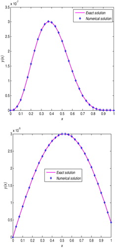
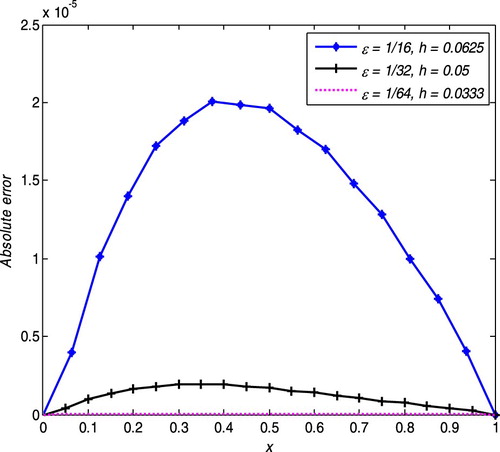
Figure 2. Absolute errors of Example 5.1 for different values of $\epsilon$ and $h$.

Example 5.2:

Consider the third order singularly perturbed boundary value problem: $\begin{array}{rl}-\epsilon y^{\mathrm{\prime }\mathrm{\prime }\mathrm{\prime }}\left(x\right)+y\left(x\right)& =81{\epsilon }^2\cos \left(3x\right)\\ & +3\epsilon \sin \left(3x\right),x\in [0,1],\end{array}$subject to, $y\left(0\right)=0,y\left(1\right)=3\epsilon \sin \left(3\right),y^{\mathrm{\prime }\mathrm{\prime }}\left(0\right)=0.$

The analytical solution of this problem is $y\left(x\right)=3\epsilon \sin \left(3x\right).$ Numerical Results are presented in Tables 3 and 4 and Figure 1.

Figure 1 shows the comparison of numerical solution and exact solution, and Figure 2 shows the absolute errors for different values of h and $\epsilon .$

6. Conclusion

The non-polynomial septic spline method is developed for the approximate solution of a third order singularly perturbed two-point boundary value problems. The convergence analysis is investigated and shows that the present method is of fourth order convergent. Two examples are considered for numerical illustration of the method. As a result, from Tables 1–4 and Figure 2, one can see that the maximum absolute error decreases as a mesh size h and also perturbation parameter $\epsilon$ decreases, which in turn shows the convergence of the computed solution. Furthermore, the result of the present method is compared with current findings and shows that it is more accurate than some existing numerical methods reported in the literature. The present method approximates the exact solution very well, Figure 1.

Moreover, the study has been analyzed by taking different mesh size h and sufficiently small perturbation parameter$\epsilon$. So, this study developed a better method for solving singularly perturbed boundary value problems for most numerical schemes fail to give good result at small mesh size $h$ and for sufficiently small perturbation parameter $\epsilon <<h$.

Generally, the present method is convergent and more accurate for solving third order singularly perturbed two point boundary value problems.

Disclosure statement

No potential conflict of interest was reported by the authors.

ORCID

Gemechis File Duresssa http://orcid.org/0000-0003-1889-4690

Gashu Gadisa Kiltu http://orcid.org/0000-0003-3541-2630

Appendix A

$\begin{array}{rl}{X}_i& =R_2{S}_{i+1}-S_2{R}_{i+1},i=1\left(1\right)15,i\ne 2\\ Z_i& =S_2{T}_{i+1}-T_2{S}_{i+1},i=2\left(1\right)15,i\ne 1\\ S_i& =\left\{\begin{array}{l}{J}_1{G}_{i+1}-G_1{J}_{i+1},i=1,2\\ J_1{G}_{i+1}-G_1{J}_i,i=4\left(1\right)7\\ J_1{G}_{i-1}-G_1{J}_{i-2},i=12,13\\ -G_1{J}_{i-2},i=14,15,16\\ -G_1{J}_i,i=8,9\\ J_1{G}_{i-1},i=3,10,11\end{array}\right.\end{array}$

$\begin{array}{rl}{H}_i& =\left\{\begin{array}{l}{A}_1{D}_{i+1}-D_1{A}_{i+1},i=1\left(1\right)4\\ A_1{D}_{i+1}-D_1{A}_i,i=6\left(1\right)10\\ A_1{D}_i,i=12,13\\ A_1{D}_i-D_1{A}_{i-2},i=14\left(1\right)17\\ -D_1{A}_i,i=11\\ -D_1{A}_i,i=18\\ A_1{D}_{i+1},i=5\end{array}\right.\\ I_i& =B_4{C}_i-C_4{B}_i,i=1\left(1\right)14\\ J_i& =\left\{\begin{array}{l}{C}_4{F}_i-F_4{C}_i,i=1\left(1\right)3\\ C_4{F}_{i+1}-F_4{C}_i,i=5\left(1\right)14\\ C_4{F}_{i+1},i=4\end{array}\right.\end{array}$ $\begin{array}{rl}{G}_1& =E_2{M}_1-M_2{E}_1\\ G_2& =E_3{M}_1-M_3{E}_1\\ G_3& =-M_4{E}_1\\ G_4& =E_4{M}_1\\ G_5& =E_5{M}_1-6E_1\\ G_6& =E_6{M}_1+18E_1\\ G_7& =E_7{M}_1-18E_1\\ G_8& =6E_1\\ G_i& =M_1{E}_{i-1},i=9\left(1\right)12\\ E_1& =U_2{W}_1-W_2{U}_1\\ E_2& =U_3{W}_1-W_3{U}_1\\ E_3& =U_4{W}_1-W_4{U}_1\\ E_4& =110W_1-42U_1\\ E_5& =-1650W_1+126U_1\\ E_6& =-990W_1-126U_1\\ E_7& =-110W_1+42U_1\\ E_8& =2640W_1,E_9=-7920W_1\\ E_{10}& =7920W_1,E_{11}=-2640W_1\\ R_i& =\left\{\begin{array}{l}{G}_1{I}_{i+1}-G_{i+1}{C}_1,i=1,2\\ -G_i{I}_i,i=3\\ G_1{I}_{i-1}-G_{i+1}{C}_1,i=5,6,7\\ G_1{I}_{i-3}-G_{i-1}{C}_1,i=12,13\\ G_1{I}_{i-1},i=8,9\\ -G_{i+1}{I}_1,i=4\\ -G_{i-1}{I}_1,i=10,11\end{array}\right.\end{array}$ $\begin{array}{rl}{O}_i& =H_i{F}_4-F_i{H}_4,i=1\left(1\right)3\\ O_i& =H_{i+1}{F}_4-F_i{H}_4,i=5\left(1\right)10\\ O_i& =H_{i+1}{F}_4-F_i{H}_{i-2},i=13\left(1\right)17\\ O_i& =H_{i+1}{F}_4,i=4,11,12\\ T_i& =\left\{\begin{array}{l}{J}_1{O}_{i+1}-O_1{J}_{i+1},i=1,2\\ J_1{O}_{i+1}-O_1{J}_i,i=4\left(1\right)9\\ J_1{O}_{i+1}-O_1{J}_{i-2},i=12\left(1\right)16\\ J_1{O}_{i+1},i=10,11\\ -O_1{J}_{i+1},i=3\end{array}\right.\end{array}$ $\begin{array}{rl}{D}_i& =W_1{K}_{i+1}-K_1{W}_{i+1}i=2\left(1\right)3\\ D_4& =K_5{W}_1,D_5=K_6{W}_1\\ D_6& =68W_1-42K_1\\ D_7& =-1536W_1+126K_1\\ D_8& =-732W_1-126K_1\\ D_9& =-68W_1+42K_1\\ D_{10}& =-384W_1,D_{11}=12W_1,\\ D_{12}& =2640W_1,D_{13}=-8640W_1,\\ D_{14}& =10800W_1,\\ D_{15}& =-6960W_1\\ D_{16}& =2880W_1,\\ D_{17}& =-720W_1\\ K_1& =-89{\alpha }_2+56{\alpha }_1+55{\alpha }_3\\ K_2& =40{\alpha }_3+56{\beta }_1\\ K_3& =89{\alpha }_2+56{\alpha }_1-55{\alpha }_3\\ K_4& =-12{\alpha }_1-21{\alpha }_2-25{\alpha }_3\\ K_5& =-12{\beta }_1\\ K_6& =21{\alpha }_2-12{\alpha }_1-15{\alpha }_3\\ N_1& =-3M_1\\ N_2& =-9{\beta }_1-9{\alpha }_1-15{\alpha }_3\\ N_3& =-9{\alpha }_2-9{\alpha }_1+40{\alpha }_3-9{\beta }_1\\ N_4& =-89{\alpha }_2-65{\alpha }_1+70{\alpha }_3\\ N_5& =-40{\alpha }_3-56{\beta }_1\\ N_6& =89{\alpha }_2-56{\alpha }_1-55{\alpha }_3\\ F_i& =A_1{M}_{i+1}-M_1{A}_{i+1}i=1\left(1\right)3\\ F_4& =-A_5{M}_1\\ F_5& =6A_1-A_6{M}_1\\ F_6& =-18A_1-A_7{M}_1\\ F_7& =18A_1-A_8{M}_1\\ F_8& =-6A_1-A_9{M}_1\\ F_i& =-M_1{A}_{i-1}i=9\left(1\right)15\end{array}$ $\begin{array}{rl}{A}_1& =N_1{P}_5,\\ A_i& =P_5{N}_i-N_6{P}_i,i=2\left(1\right)5\\ A_6& =-18P_5,\\ A_7& =66P_5+8N_6\\ A_8& =202P_5-20N_6\\ A_9& =-702P_5+132N_6\\ A_{10}& =-1536P_5+124N_6\\ A_{11}& =68P_5-4N_6,A_{12}=-720P_5,\\ A_{13}& =4800P_5-240N_6\\ A_{14}& =-10080P_5+720N_6\\ A_{15}& =8640P_5-720N_6\\ A_{16}& =-2640P_5+240N_6\\ B_i& =Q_i{P}_5-P_i{Q}_5,i=1\left(1\right)4\\ B_5& =-4P_5+8Q_5\\ B_6& =128P_5-20Q_5\\ B_7& =132Q_5\\ B_8& =-128P_5+124Q_5\\ B_9& =4P_5-4Q_5\\ B_{10}& =-240P_5\\ B_{11}& =960P_5-240Q_5\\ B_{12}& =-1440P_5+720Q_5\\ B_{13}& =960P_5-720Q_5\\ B_{14}& =-240P_5+240Q_5\\ C_1& =-Q_1{L}_4\\ C_i& =L_{i-1}{Q}_5-Q_i{L}_4,i=2\left(1\right)4\\ C_5& =4L_4\\ C_6& =-110Q_5-128L_4\\ C_7& =-990Q_5\\ C_8& =-1650Q_5+128L_4\\ C_9& =110Q_5-4L_4\\ C_{10}& =240L_4\\ C_{11}& =2640Q_5-960L_4\\ C_{12}& =-7920Q_5+1440L_4\\ C_{13}& =7920Q_5-960L_4\\ C_{14}& =-2640Q_5+240L_4\end{array}$ $\begin{array}{rl}{M}_1& =-3{\alpha }_2+3{\alpha }_1\\ M_2& =3{\alpha }_2+3{\alpha }_1+3{\beta }_1\\ M_3& =M_2\\ M_4& =M_1\\ W_1& =7M_1\\ W_2& =7M_2\\ W_3& =W_2\\ W_4& =W_1\\ U_1& =-110{\alpha }_2+77{\alpha }_1+55{\alpha }_3\\ U_2& =33{\alpha }_1+55{\alpha }_3+77{\beta }_1\\ U_3& =110{\alpha }_2+77{\alpha }_1-55{\alpha }_3+33{\beta }_1\\ U_4& =33{\alpha }_1-55{\alpha }_3\\ L_1& =-U_4\\ L_2& =-U_3\\ L_3& =-U_2\\ L_4& =-U_1\\ P_1& =4{\alpha }_2-4{\alpha }_1\\ P_2& =-7{\alpha }_2-4{\alpha }_1+5{\alpha }_3-4{\beta }_1\\ P_3& =-11{\alpha }_2-8{\alpha }_1+5{\alpha }_3-4{\beta }_1\\ P_4& =7{\alpha }_2-4{\alpha }_1-5{\alpha }_3-4{\beta }_1\\ P_5& =7{\alpha }_2-4{\alpha }_1-5{\alpha }_3\\ Q_1& =P_5\\ Q_2& =-4{\beta }_1\\ Q_3& =-14{\alpha }_2-8{\alpha }_1+10{\alpha }_3\\ Q_4& =Q_2\\ Q5& =P_5\end{array}$

References

- Priyadharshini RM, Ramanujam N. Approximation of derivative to a singularly perturbed second-order ordinary differential equation with discontinuous convection coefficient using hybrid difference scheme. Int J Comput Math. 2009;86(8):1355–1365. doi: 10.1080/00207160701870837
- Rashidinia J, Mohammadi R, Moatamedoshariati SH. Quintic spline methods for the solution of singularly perturbed boundary-value problems. Int J Comput Meth Eng Sci Mech. 2010;11:247–257. doi: 10.1080/15502287.2010.501321
- Akram G. Quartic spline solution of third order singularly perturbed boundary value problem. Anzaim J. 2012;53(E):E44–E58. doi: 10.21914/anziamj.v53i0.4526
- Christy RJ, Tamilselvan A. Numerical method for singularly perturbed third order ordinary differential equations of reaction-diffusion type. J Appl Math and Informatics. 2017;35(3–4):277–302.
- Mustafa G, Ejaz ST. A subdivision collocation method for solving two point boundary value problems of order three. J Appl Anal Comput. 2017;7(3):942–956.
- Yohannis AW, Gemechis FD, Tesfaye AB. Quintic non-polynomial spline methods for third order singularly perturbed boundary value problems. JKSUS. 2018;30:131–137.
- Battal GK, Halil Z, Turgut AK. Numerical solution of the Kawahara equation by the septic B-spline collocation method. Soic. 2014;2(3):211–221.
- Turgut AK, Sharanjeet D, Bilge I. Numerical solutions of generalized Rosenau-Kawahara-RLW equation arising in fluid mechanics via B-spline collocation method. IJMPC. 2018;29(11):1850116. doi: 10.1142/S0129183118501164
- Aka T, Trikib H, Dhawanc S, et al. Computational analysis of shallow water waves with Korteweg-de Vries equation. Scientia Iranica B. 2018;25(5):2582–2597.
- Khan A, Khandelwal P. Non-polynomial sextic spline solution of singularly perturbed boundary value problems. Int J Comput Math. 2014;91(5):1122–1135. doi: 10.1080/00207160.2013.828865
- Akram G, Siddiqi S. End conditions for interpolatory septic splines. Int J Comput Math. 2005;82:1525–1540. doi: 10.1080/00207160412331291099
- Mohanty RK, Jha N. A class of variable mesh spline in compression methods for singularly perturbed two point singular boundary value problems. Appl Math Comput. 2005;168(1):704–716.
- Akram G, Talib I. Quartic non-polynomial spline solution of a third order singularly perturbed boundary value problem. Res J Appl Sci Eng Tech. 2014;7(23):4859–4863. doi: 10.19026/rjaset.7.875