Reproducing kernel Hilbert space method for the solutions of generalized Kuramoto–Sivashinsky equation

Abstract

Reproducing kernel Hilbert space method is given for the solution of generalized Kuramoto–Sivashinsky equation. Reproducing kernel functions are obtained to get the solution of the generalized Kuramoto–Sivashinsky equation. Two examples have been introduced to prove the accuracy of the method. The obtained results show that the reproducing kernel Hilbert space method gives approximate analytical solutions which are very close to the exact solution of the generalized Kuramoto–Sivashinsky equation, which demonstrates the power of the proposed technique. We prove the efficiency of the reproducing kernel Hilbert space method in this paper.

Keywords:

• Generalized Kuramoto–Sivashinsky equation
• reproducing kernel functions
• Hilbert spaces

2000 Mathematics Subject Classifications:

• 46E20
• 46E22
• 35G20

1. Introduction

The generalized Kuramoto–Sivashinsky equation is a model of nonlinear partial differential equation which encountered in the work of continuous media [1]. We investigate this equation by reproducing kernel Hilbert space method: (1) $\frac{\mathrm{\partial }s}{\mathrm{\partial }t}+s\frac{\mathrm{\partial }s}{\mathrm{\partial }x}+\alpha \frac{{\mathrm{\partial }}^{2}s}{\mathrm{\partial }{x}^2}+\beta \frac{{\mathrm{\partial }}^{3}s}{\mathrm{\partial }{x}^3}+\gamma \frac{{\mathrm{\partial }}^{4}s}{\mathrm{\partial }{x}^4}=0,$(1) where α, β and γ are non-zero [2,3].

Equation (1(1) $\frac{\mathrm{\partial }s}{\mathrm{\partial }t}+s\frac{\mathrm{\partial }s}{\mathrm{\partial }x}+\alpha \frac{{\mathrm{\partial }}^{2}s}{\mathrm{\partial }{x}^2}+\beta \frac{{\mathrm{\partial }}^{3}s}{\mathrm{\partial }{x}^3}+\gamma \frac{{\mathrm{\partial }}^{4}s}{\mathrm{\partial }{x}^4}=0,$(1) ) is called the Kuramoto–Sivashinsky equation for $\beta =0.$ This equation emerges in the context of long waves on the interface between two viscous fluids [4], unstable drift waves in plasmas, and flame front instability [5]. This equation is practical to model solitary pulses in a falling thin film [6].

For $\alpha =\gamma =1$ and $\beta =0$ it gives models of pattern formation on unstable flame fronts and thin hydrodynamic films. Therefore, Equation (1(1) $\frac{\mathrm{\partial }s}{\mathrm{\partial }t}+s\frac{\mathrm{\partial }s}{\mathrm{\partial }x}+\alpha \frac{{\mathrm{\partial }}^{2}s}{\mathrm{\partial }{x}^2}+\beta \frac{{\mathrm{\partial }}^{3}s}{\mathrm{\partial }{x}^3}+\gamma \frac{{\mathrm{\partial }}^{4}s}{\mathrm{\partial }{x}^4}=0,$(1) ) has been investigated by many researchers [7,8].

Many techniques have been given to investigate this equation recently. This equation is investigated by lattice Boltzmann technique in [9]. The method of radial basis functions [10,11] has been enhanced in [12] to obtain the approximate solution of this equation. The local discontinuous Galerkin methods have been used to search this equation in [13]. The tanh function method has been proposed in [14].

Reproducing kernel Hilbert space method is very powerful method. There are many advantages of this method. We can obtain approximate solutions of the problems in a short time by this method. The approximate solutions to the equations have been computed by using the RKHSM without any need to transformation techniques and linearization or perturbation of the equations. The RKHSM avoids the difficulties and massive computational work by determining the analytic solutions.

Reproducing kernels were used for the first time at the beginning of the twentieth century [15,16]. Geng [17] have applied a new reproducing kernel Hilbert space method for solving nonlinear fourth-order boundary value problems. Zhang et al. [18] have found reproducing kernel functions represented by form of polynomials. Gumah et al. [19] have investigated the solutions of uncertain Volterra integral equations by fitted reproducing kernel Hilbert space method. Saadeh et al. [20] have studied the numerical investigation for solving two-point fuzzy boundary value problems by reproducing kernel approach. Arqub et al. [21] have found numerical solutions of fuzzy differential equations using reproducing kernel Hilbert space method. Hashemi et al. [22] have solved the Lane–Emden equation within a reproducing kernel method and group preserving scheme. Arqub et al. [23] have found the numerical solutions of fractional differential equations of Lane–Emden type by an accurate technique. For more details see [24–28].

We organize our paper as: In Section 2 some useful reproducing kernel functions are obtained. In Section 3 reproducing kernel Hilbert space method is applied to find the solution of the generalized Kuramoto–Sivashinsky equation. Numerical results have been shown in Section 4. Conclusion is given in the final section.

2. Some useful reproducing kernel functions

We need the following reproducing kernel Hilbert spaces to obtain the solution of Equation (1(1) $\frac{\mathrm{\partial }s}{\mathrm{\partial }t}+s\frac{\mathrm{\partial }s}{\mathrm{\partial }x}+\alpha \frac{{\mathrm{\partial }}^{2}s}{\mathrm{\partial }{x}^2}+\beta \frac{{\mathrm{\partial }}^{3}s}{\mathrm{\partial }{x}^3}+\gamma \frac{{\mathrm{\partial }}^{4}s}{\mathrm{\partial }{x}^4}=0,$(1) ). We find very useful reproducing kernel functions in these spaces.

Definition 2.1

$V_2^1[0,1]$ is a reproducing kernel Hilbert space. We define this space as: (2) $V_2^1[0,1]=\{\eta \in AC[0,1]:{\eta }^{\prime }\in L^2[0,1\left]\right\},$(2) where AC defines the absolutely continuous functions. We have the inner product and norm for this space as: (3) ${⟨\eta ,y⟩}_{V_2^1}=\eta \left(0\right)y\left(0\right)+{\int }_0^1{\eta }^{\prime }\left(\theta \right)y^{\prime }\left(\theta \right)\mathrm{d}\theta .$(3) We find the reproducing kernel function $m_t$ of this space as ([29], pp. 10 and 17): (4) $m_t\left(\theta \right)=\left\{\begin{array}{ll}1+\theta ,& 0\le \theta \le t\le 1,\\ 1+t,& 0\le t<\theta \le 1.\end{array}\right.$(4)

Definition 2.2

$V_2^2[0,1]$ is a reproducing kernel Hilbert space. We define this space as: (5) $V_2^2[0,1]=\{\eta \in AC[0,1]:{\eta }^{\mathrm{\prime }}\in AC[0,1],{\eta }^{″}\in L^2[0,1\left]\right\}.$(5) We construct the inner product and norm in this space as: (6) $\begin{array}{rl}{⟨\eta ,y⟩}_{V_2^2[0,1]}& =\eta \left(0\right)y\left(0\right)+{\eta }^{\prime }\left(0\right)y^{\prime }\left(0\right)\\ & +{\int }_0^1{\eta }^{″}\left(\theta \right)y^{″}\left(\theta \right)\mathrm{d}\theta ,\eta ,y\in V_2^2[0,1],\end{array}$(6) and (7) ${∥\eta ∥}_{V_2^2[0,1]}=\sqrt{{⟨\eta ,\eta ⟩}_{V_2^2[0,1]}},\eta \in V_2^2[0,1].$(7) We find the reproducing kernel function $n_x$ of this space as [29]: (8) $n_x\left(\beta \right)=\left\{\begin{array}{ll}1+\beta x+\frac{1}{2}x{\beta }^2-\frac{{\beta }^3}{6},& 0\le \beta \le x\le 0,\\ 1+\beta x+\frac{1}{2}{x}^2\beta -\frac{x^3}{6},& 0\le x<\beta \le 1.\end{array}\right.$(8)

Definition 2.3

${}^0{V}_2^2[0,1]$ is also a reproducing kernel Hilbert space. We need this special space for domain. We define this space as: (9) $\begin{array}{rl}{}^0{V}_2^2[0,1]& =\{\eta \in AC[0,1]:{\eta }^{\mathrm{\prime }}\in AC[0,1],\\ {\eta }^{″}& \in L^2[0,1],\eta \left(0\right)=0\}.\end{array}$(9) We describe the inner product and the norm of this space by: (10) $\begin{array}{rl}{⟨\eta ,y⟩}_{{}^0{V}_2^2[0,1]}& =\eta \left(0\right)y\left(0\right)+{\eta }^{\prime }\left(0\right)y^{\prime }\left(0\right)\\ & +{\int }_0^1{\eta }^{″}\left(\theta \right)y^{″}\left(\theta \right)\mathrm{d}\theta ,\eta ,y\in {}^0{V}_2^2[0,1],\end{array}$(10) and (11) ${∥\eta ∥}_{{}^0{V}_2^2[0,1]}=\sqrt{{⟨\eta ,\eta ⟩}_{{}^0{V}_2^2[0,1]}},\eta {\in }^0{V}_2^2[0,1].$(11)

We find the reproducing kernel function $N_x$ of this reproducing kernel Hilbert space as [29]: (12) $N_x\left(\beta \right)=\left\{\begin{array}{ll}\beta x+\frac{1}{2}x{\beta }^2-\frac{{\beta }^3}{6},& 0\le \beta \le x\le 0,\\ \beta x+\frac{1}{2}{x}^2\beta -\frac{x^3}{6},& 0\le x<\beta \le 1.\end{array}\right.$(12)

Definition 2.4

${}^0{V}_2^5[0,1]$ is a reproducing kernel Hilbert space. We need this space also for domain. We define this special Hilbert space by: (13) $\begin{array}{rl}& {}^0{V}_2^5[0,1]\\ & =\left\{\begin{array}{c}v,v^{\prime },v^{″},v^{‴},v^{\left(4\right)}\\ \mathrm{a}\mathrm{r}\mathrm{e}\mathrm{a}\mathrm{b}\mathrm{s}\mathrm{o}\mathrm{l}\mathrm{u}\mathrm{t}\mathrm{e}\mathrm{l}\mathrm{y}\mathrm{c}\mathrm{o}\mathrm{n}\mathrm{t}\mathrm{i}\mathrm{n}\mathrm{u}\mathrm{o}\mathrm{u}\mathrm{s}\mathrm{f}\mathrm{u}\mathrm{n}\mathrm{c}\mathrm{t}\mathrm{i}\mathrm{o}\mathrm{n}\mathrm{s}\mathrm{i}\mathrm{n}[0,1]\\ v^{\left(5\right)}\in L^2[0,1],\\ v\left(0\right)=v^{\prime }\left(0\right)=v\left(1\right)=v^{\prime }\left(0\right)=0.\end{array}\right\}\end{array}$(13) We present the inner product and norm for this space as: $\begin{array}{rl}⟨\eta ,y{⟩}_{V_2^5[0,1]}& =\eta \left(0\right)y\left(0\right)+{\eta }^{\prime }\left(0\right)y^{\prime }\left(0\right)\\ & +{\eta }^{″}\left(0\right)y^{″}\left(0\right)+{\eta }^{‴}\left(0\right)y^{‴}\left(0\right)\\ & +{\eta }^{\left(4\right)}\left(0\right)y^{\left(4\right)}\left(0\right)+{\int }_0^1{\eta }^{\left(5\right)}\left(\theta \right)y^{\left(5\right)}\left(\theta \right)\mathrm{d}\left(\theta \right),\end{array}$ and ${∥\eta ∥}_{{}^0{V}_2^5[0,1]}=\sqrt{{⟨\eta ,\eta ⟩}_{{}^0{V}_2^5[0,1]}},\eta \in {}^0{V}_2^5[0,1].$

Theorem 2.5

Reproducing kernel function $M_t$ of reproducing kernel Hilbert space ${}^0{V}_2^5[0,1]$ is obtained as for $t\le \theta$:

$\begin{array}{rl}{M}_t\left(\theta \right)& =\frac{7198143016396640625}{1009990080344}t+\frac{7198143016396640625}{1009990080344}\theta -\frac{236233133659}{4188630861202636800}{t}^9\theta \\ & -\frac{25577335706625000}{126248760043}{\theta }^2-\frac{48269392667}{104715771530065920}{\theta }^9+\frac{17966234381625}{1154274377536}{\theta }^5\\ & +\frac{29272459010625}{577137188768}{\theta }^4-\frac{2676222488053125}{144284297192}{\theta }^3+\frac{2246464475}{1154274377536}{\theta }^6\\ & -\frac{80748516375}{16159841285504}{\theta }^7+\frac{32209547971}{387836190852096}{\theta }^8+\frac{56794291302308203125}{504995040172}\\ & +\frac{123372139067}{11635085725562880}t{\theta }^8+\frac{4216064564110078125}{8079920642752}t\theta -\frac{18660702648290625}{2019980160688}t{\theta }^2\\ & -\frac{236233133659}{4188630861202636800}t{\theta }^9+\frac{11410798339425}{9234195020288}t{\theta }^5-\frac{1056580144875}{144284297192}t{\theta }^4\\ & -\frac{1582454023284375}{1154274377536}t{\theta }^3+\frac{52555722375}{4617097510144}t{\theta }^6-\frac{278277711559}{387836190852096}t{\theta }^7\\ & -\frac{56066836171}{1454385715695360}{t}^2{\theta }^7-\frac{271343642075}{288568594384}{t}^2{\theta }^4+\frac{7614132262875}{288568594384}{t}^2{\theta }^3\\ & +\frac{78589676998125}{126248760043}{t}^2{\theta }^2-\frac{18660702648290625}{2019980160688}{t}^2\theta +\frac{4879103003}{10907892867715200}{t}^2{\theta }^8\\ & +\frac{5678004049}{3462823132608}{t}^2{\theta }^6-\frac{60346062085}{2308548755072}{t}^2{\theta }^5-\frac{444730933}{209431543060131840}{t}^2{\theta }^9\\ & +\frac{8010566353}{89044023409920}{t}^3{\theta }^6+\frac{1106637555}{82448169824}{t}^3{\theta }^4+\frac{1920514145375}{494689018944}{t}^3{\theta }^3\\ & +\frac{7614132262875}{288568594384}{t}^3{\theta }^2-\frac{1582454023284375}{1154274377536}{t}^3\theta +\frac{1379065}{332431020730368}{t}^3{\theta }^8\\ & -\frac{11113462603}{12466163277388800}{t}^3{\theta }^7-\frac{6976267603}{1319170717184}{t}^3{\theta }^5-\frac{1298122397}{403903690187397120000}{t}^3{\theta }^9\end{array}$ $\begin{array}{rl}& -\frac{57787325}{329792679296}{t}^4{\theta }^5+\frac{25991263693}{5936268227328}{t}^4{\theta }^4+\frac{1106637555}{82448169824}{t}^4{\theta }^3\\ & -\frac{271343642075}{288568594384}{t}^4{\theta }^2-\frac{1056580144875}{144284297192}{t}^4\theta -\frac{627953}{3989172248764416}{t}^4{\theta }^8\\ & -\frac{494407}{83107755182592}{t}^4{\theta }^7+\frac{25586965}{11872536454656}{t}^4{\theta }^6+\frac{908543}{673172816978995200}{t}^4{\theta }^9\\ & +\frac{2552580989}{14840670568320}{t}^5{\theta }^4+\frac{231241}{13297240829214720000}{t}^5{\theta }^9-\frac{20227}{7978344497528832}{t}^5{\theta }^8\\ & +\frac{1496479}{33243102073036800}{t}^5{\theta }^7+\frac{1186757}{79150243031040}{t}^5{\theta }^6-\frac{15737563}{10553365737472}{t}^5{\theta }^5\\ & -\frac{6976267603}{1319170717184}{t}^5{\theta }^3-\frac{60346062085}{2308548755072}{t}^5{\theta }^2+\frac{11410798339425}{9234195020288}{t}^5\theta \\ & -\frac{12601476103}{89044023409920}{t}^6{\theta }^3-\frac{4008157}{24234221411243827200000}{t}^6{\theta }^9+\frac{14107}{598375837314662400}{t}^6{\theta }^8\\ & -\frac{223943}{747969796643328000}{t}^6{\theta }^7-\frac{417041}{2671320702297600}{t}^6{\theta }^6+\frac{1186757}{79150243031040}{t}^6{\theta }^5\\ & +\frac{25586965}{11872536454656}{t}^6{\theta }^4+\frac{5678004049}{3462823132608}{t}^6{\theta }^2+\frac{52555722375}{4617097510144}{t}^6\theta \\ & +\frac{88217461021}{1454385715695360}{t}^7{\theta }^2-\frac{2697893}{3392790997574135808000000}{t}^7{\theta }^9+\frac{16493}{125658925836079104000}{t}^7{\theta }^8\\ & -\frac{600707}{104715771530065920000}{t}^7{\theta }^7-\frac{223943}{747969796643328000}{t}^7{\theta }^6+\frac{1496479}{33243102073036800}{t}^7{\theta }^5\\ & -\frac{494407}{83107755182592}{t}^7{\theta }^4-\frac{11113462603}{12466163277388800}{t}^7{\theta }^3-\frac{278277711559}{387836190852096}{t}^7\theta \\ & -\frac{165196455317}{11635085725562880}{t}^8\theta -\frac{75307}{15079071100329492480000}{t}^8{\theta }^8+\frac{16493}{125658925836079104000}{t}^8{\theta }^7\\ & +\frac{14107}{598375837314662400}{t}^8{\theta }^6-\frac{20227}{7978344497528832}{t}^8{\theta }^5-\frac{627953}{3989172248764416}{t}^8{\theta }^4\end{array}$ $\begin{array}{rl}& +\frac{1379065}{332431020730368}{t}^8{\theta }^3+\frac{4879103003}{10907892867715200}{t}^8{\theta }^2+\frac{44707}{1357116399029654323200000}{t}^8{\theta }^9\\ & -\frac{24126307}{109926428321402000179200000000}{t}^9{\theta }^9+\frac{44707}{1357116399029654323200000}{t}^9{\theta }^8\\ & -\frac{2697893}{3392790997574135808000000}{t}^9{\theta }^7-\frac{4008157}{24234221411243827200000}{t}^9{\theta }^6\\ & +\frac{908543}{673172816978995200}{t}^9{\theta }^4-\frac{1298122397}{403903690187397120000}{t}^9{\theta }^3-\frac{444730933}{209431543060131840}{t}^9{\theta }^2\\ & -\frac{25577335706625000}{126248760043}{t}^2-\frac{2676222488053125}{144284297192}{t}^3+\frac{29272459010625}{577137188768}{t}^4\\ & +\frac{17966234381625}{1154274377536}{t}^5+\frac{2246464475}{1154274377536}{t}^6-\frac{80748516375}{16159841285504}{t}^7\\ & +\frac{32209547971}{387836190852096}{t}^8+\frac{240299201717}{104715771530065920}{t}^9+\frac{231241}{13297240829214720000}{t}^9{\theta }^5.\end{array}$

Proof.

We get $\begin{array}{rl}& ⟨\eta ,M_t{⟩}_{{}^0{V}_2^5[0,1]}\\ & =\eta \left(0\right)M_t\left(0\right)+{\eta }^{\prime }\left(0\right)M_t^{\mathrm{\prime }}\left(0\right)\\ & +{\eta }^{″}\left(0\right)M_t^{″}\left(0\right)+{\eta }^{‴}\left(0\right)M_t^{‴}\left(0\right)\\ & +{\eta }^{\left(4\right)}\left(0\right)M_t^{\left(4\right)}\left(0\right)+{\eta }^{\left(4\right)}\left(1\right)M_t^{\left(5\right)}\left(1\right)\\ & -{\eta }^{\left(4\right)}\left(0\right)M_t^{\left(5\right)}\left(0\right)\\ & -{\eta }^{\left(3\right)}\left(1\right)M_t^{\left(6\right)}\left(1\right)+{\eta }^{\left(3\right)}\left(0\right)M_t^{\left(6\right)}\left(0\right)\\ & +{\eta }^{″}\left(1\right)M_t^{\left(7\right)}\left(1\right)-{\eta }^{″}\left(0\right)M_t^{\left(7\right)}\left(0\right)-{\eta }^{\prime }\left(1\right)M_t^{\left(8\right)}\left(1\right)\\ & +{\eta }^{\prime }\left(0\right)M_t^{\left(8\right)}\left(0\right)+\eta \left(1\right)M_t^{\left(9\right)}\left(1\right)-\eta \left(0\right)M_t^{\left(9\right)}\left(0\right)\\ & -{\int }_0^1\eta \left(\theta \right)M_t^{\left(10\right)}\left(\theta \right)\mathrm{d}\theta .\end{array}$ by Definition 2.4 and integration by parts. Since $M_t\in {}^0{V}_2^5[0,1]$, we can write $\begin{array}{rl}{M}_t\left(0\right)& =0\\ M_t\left(1\right)& =0\\ M_t^{\prime }\left(0\right)& =0\\ M_t^{\prime }\left(1\right)& =0.\end{array}$ Then, we obtain $\begin{array}{rl}& ⟨\eta ,M_t{⟩}_{{}^0{V}_2^5[0,1]}\\ & ={\eta }^{″}\left(0\right)M_t^{″}\left(0\right)+{\eta }^{‴}\left(0\right)M_t^{‴}\left(0\right)+{\eta }^{\left(4\right)}\left(0\right)M_t^{\left(4\right)}\left(0\right)\\ & +{\eta }^{\left(4\right)}\left(1\right)M_t^{\left(5\right)}\left(1\right)-{\eta }^{\left(4\right)}\left(0\right)M_t^{\left(5\right)}\left(0\right)-{\eta }^{\left(3\right)}\left(1\right)M_t^{\left(6\right)}\left(1\right)\\ & +{\eta }^{\left(3\right)}\left(0\right)M_t^{\left(6\right)}\left(0\right)+{\eta }^{″}\left(1\right)M_t^{\left(7\right)}\left(1\right)-{\eta }^{″}\left(0\right)M_t^{\left(7\right)}\left(0\right)\\ & -{\int }_0^1\eta \left(t\right)M_t^{\left(10\right)}\left(\theta \right)\mathrm{d}\theta .\end{array}$ If we have $\begin{array}{rl}{M}_t^{″}\left(0\right)-M_t^{\left(7\right)}\left(0\right)& =0\\ M_t^{‴}\left(0\right)+M_t^{\left(6\right)}\left(0\right)& =0\\ M_t^{\left(4\right)}\left(0\right)-M_t^{\left(5\right)}\left(0\right)& =0\\ M_t^{\left(5\right)}\left(1\right)& =0\\ M_t^{\left(6\right)}\left(1\right)& =0\\ M_t^{\left(7\right)}\left(1\right)& =0,\end{array}$ then, we will get $⟨\eta ,M_t{⟩}_{{}^0{V}_2^5[0,1]}=-{\int }_0^1\eta \left(\theta \right)M_t^{\left(10\right)}\left(\theta \right)\mathrm{d}\theta =\eta \left(t\right).$ Therefore, we can write $M_t^{\left(10\right)}\left(\theta \right)=-\delta (\theta -t).$ We know that when $\theta \ne t,$ we have $M_t^{\left(10\right)}\left(z\right)=0.$ Thus, we reach $M_t\left(\theta \right)=\left\{\begin{array}{ll}\sum _{i=1}^{10}{c}_i\left(t\right){\theta }^{i-1},& \theta \le t,\\ \sum _{i=1}^{10}{d}_i\left(t\right){\theta }^{i-1},& \theta >t.\end{array}\right.$ The unknown conditions can be obtained by the above equations easily. This completes the proof.

Definition 2.6

We need the binary reproducing kernel Hilbert spaces to solve the partial differential equations by reproducing kernel Hilbert space method. Our first binary reproducing kernel Hilbert space $V\left(D\right)$, where $D=[0,1]\times [0,1]$, is given as [29]: $\begin{array}{rl}V\left(D\right)& =\left\{\eta :\frac{{\mathrm{\partial }}^5\eta }{\mathrm{\partial }{x}^4\mathrm{\partial }t}\in CC\left(D\right),\frac{{\mathrm{\partial }}^7\eta }{\mathrm{\partial }{x}^5\mathrm{\partial }{t}^2}\in L^2\left(D\right),\right.\\ & \left.\phantom{\frac{{\mathrm{\partial }}^5\eta }{\mathrm{\partial }{x}^4\mathrm{\partial }t}}\eta (x,0)=\eta (0,t)=\eta (1,t)={\eta }^{\prime }(0,t)={\eta }^{\prime }(1,t)=0\right\},\end{array}$ where CC defines the space of completely continuous functions.

We have the inner product and the norm for this space as [29]: $\begin{array}{rl}& {⟨\eta ,y⟩}_{V\left(D\right)}\\ & =\sum _{i=0}^4{\int }_0^1\left[\frac{{\mathrm{\partial }}^2}{\mathrm{\partial }{t}^2}\frac{{\mathrm{\partial }}^i}{\mathrm{\partial }{x}^i}\eta (0,t)\frac{{\mathrm{\partial }}^2}{\mathrm{\partial }{t}^2}\frac{{\mathrm{\partial }}^i}{\mathrm{\partial }{x}^i}y(0,t)\right]\mathrm{d}t\\ & +\sum _{j=0}^1{⟨\frac{{\mathrm{\partial }}^j}{\mathrm{\partial }{t}^j}\eta (\cdot ,0),\frac{{\mathrm{\partial }}^j}{\mathrm{\partial }{t}^j}y(\cdot ,0)⟩}_{{}^0{V}_2^2[0,1]}\\ & +{\int }_0^1{\int }_0^1\left[\frac{{\mathrm{\partial }}^5}{\mathrm{\partial }{x}^5}\frac{{\mathrm{\partial }}^2}{\mathrm{\partial }{t}^2}\eta (x,t)\frac{{\mathrm{\partial }}^5}{\mathrm{\partial }{x}^5}\frac{{\mathrm{\partial }}^2}{\mathrm{\partial }{t}^2}y(x,t)\right]\mathrm{d}t\mathrm{d}x,\\ & \times \eta ,y\in V\left(D\right)\end{array}$ and ${∥\eta ∥}_{V\left(D\right)}=\sqrt{{⟨\eta ,\eta ⟩}_{V\left(D\right)}},\eta \in V\left(D\right).$

Lemma 2.7

$V\left(D\right)$ is a binary reproducing kernel Hilbert space and $A_{(t,x)}$ is the reproducing kernel function of this space. We find $A_{(t,x)}$ by [29]: $A_{(t,x)}=M_t\left(\theta \right)N_x\left(\beta \right).$

Definition 2.8

The second binary reproducing kernel Hilbert space that we need is $\hat{V}\left(D\right).$ We define this space as: (14) $\hat{V}\left(D\right)=\left\{\eta \in CC\left(D\right),\frac{\mathrm{\partial }\zeta }{\mathrm{\partial }x}\in CC\left(D\right):\frac{{\mathrm{\partial }}^3\eta }{\mathrm{\partial }{x}^2\mathrm{\partial }t}\in L^2\left(D\right)\right\}.$(14) We define the inner product and norm of this space as [29]: $\begin{array}{rl}& {⟨\eta ,y⟩}_{\hat{V}\left(D\right)}\\ & =\sum _{i=0}^1{\int }_0^1\left[\frac{\mathrm{\partial }}{\mathrm{\partial }t}\frac{{\mathrm{\partial }}^i}{\mathrm{\partial }{x}^i}\eta (0,t)\frac{\mathrm{\partial }}{\mathrm{\partial }t}\frac{{\mathrm{\partial }}^i}{\mathrm{\partial }{x}^i}y(0,t)\right]\mathrm{d}t\\ & +{⟨\eta (\cdot ,0),y(\cdot ,0)⟩}_{V_2^1[0,1]}\\ & +{\int }_0^1{\int }_0^1\left[\frac{{\mathrm{\partial }}^2}{\mathrm{\partial }{x}^2}\frac{\mathrm{\partial }}{\mathrm{\partial }t}\eta (x,t)\frac{{\mathrm{\partial }}^2}{\mathrm{\partial }{x}^2}\frac{\mathrm{\partial }}{\mathrm{\partial }t}\eta (x,t)\right]\mathrm{d}t\mathrm{d}x,\\ & \times \eta ,y\in \hat{V}\left(D\right)\end{array}$ and ${∥\eta ∥}_{\hat{V}\left(D\right)}=\sqrt{{⟨\eta ,\eta ⟩}_{\hat{V}\left(D\right)}},\eta \in \hat{V}\left(D\right).$

Lemma 2.9

We find the reproducing kernel function $B_{(t,x)}$ of this binary reproducing kernel Hilbert space as [29]: (15) $B_{(t,x)}=m_t\left(\theta \right)n_x\left(\beta \right).$(15)

3. Application of the reproducing kernel Hilbert space method

We find the solution of Equation (1(1) $\frac{\mathrm{\partial }s}{\mathrm{\partial }t}+s\frac{\mathrm{\partial }s}{\mathrm{\partial }x}+\alpha \frac{{\mathrm{\partial }}^{2}s}{\mathrm{\partial }{x}^2}+\beta \frac{{\mathrm{\partial }}^{3}s}{\mathrm{\partial }{x}^3}+\gamma \frac{{\mathrm{\partial }}^{4}s}{\mathrm{\partial }{x}^4}=0,$(1) ) in the reproducing kernel Hilbert space $V\left(D\right).$ We describe the bounded linear operator (16) $T:V\left(D\right)\to \hat{V}\left(D\right)$(16) by (17) $Ts=\frac{\mathrm{\partial }s}{\mathrm{\partial }t}+\alpha \frac{{\mathrm{\partial }}^{2}s}{\mathrm{\partial }{x}^2}+\beta \frac{{\mathrm{\partial }}^{3}s}{\mathrm{\partial }{x}^3}+\gamma \frac{{\mathrm{\partial }}^{4}s}{\mathrm{\partial }{x}^4}.$(17) Then, our problem can be written by: (18) $Ts=K(x,t,s).$(18) We take a countable dense subset $\left\{\right(t_1,x_1),(t_2,x_2),\dots \}$ in D and present (19) $a_i=B_{(t_i,x_i)},b_i=T^{\ast }{a}_i,$(19) where $T^{\ast }$ means the adjoint operator of T. The orthonormal system $\{{\hat{b}}_i{\}}_{i=1}^{\mathrm{\infty }}$ of $V\left(D\right)$ can be found by the operation of Gram–Schmidt orthogonalization of $\{b_i{\}}_{i=1}^{\mathrm{\infty }}$ as: (20) ${\hat{b}}_i=\sum _{k=1}^i{\beta }_{ik}{b}_k.$(20)

Theorem 3.1

If $\left\{\right(t_i,x_i){\}}_{i=1}^{\mathrm{\infty }}$ is dense in D, then the solution of Equation (18(18) $Ts=K(x,t,s).$(18) ) can be found by the proposed technique as: (21) $s=\sum _{i=1}^{\mathrm{\infty }}\sum _{k=1}^i{\beta }_{ik}K(t_k,x_k,s_k){\hat{b}}_i.$(21)

Proof.

Since $\{b_i{\}}_{i=1}^{\mathrm{\infty }}$ is a complete system in $V\left(D\right),$ we get: $s=\sum _{i=1}^{\mathrm{\infty }}{⟨s,{\hat{b}}_i⟩}_{V\left(D\right)}{\hat{b}}_i=\sum _{i=1}^{\mathrm{\infty }}\sum _{k=1}^i{\beta }_{ik}{⟨s,b_k⟩}_{V\left(D\right)}{\hat{b}}_i.$ Then, we acquire $\begin{array}{rl}s& =\sum _{i=1}^{\mathrm{\infty }}\sum _{k=1}^i{\beta }_{ik}{⟨s,T^{\ast }{a}_k⟩}_{V\left(D\right)}\\ {\hat{b}}_i& =\sum _{i=1}^{\mathrm{\infty }}\sum _{k=1}^i{\beta }_{ik}{⟨Ts,a_k⟩}_{\hat{V}\left(D\right)}{\hat{b}}_i.\end{array}$ by using the feature of the adjoint operator $T^{\ast }$. We obtain $\begin{array}{rl}s& =\sum _{i=1}^{\mathrm{\infty }}\sum _{k=1}^i{\beta }_{ik}{⟨Ts,B_{(t_k,x_k)}⟩}_{\widehat{V\left(D\right)}}\\ {\hat{b}}_i& =\sum _{i=1}^{\mathrm{\infty }}\sum _{k=1}^i{\beta }_{ik}Ts(t_k,x_k){\hat{b}}_i\end{array}$ by implementing the reproducing property. Therefore, the desire result is found as: $s=\sum _{i=1}^{\mathrm{\infty }}\sum _{k=1}^i{\beta }_{ik}K(t_k,x_k,s_k){\hat{b}}_i.$ This completes the proof.

The approximate solution $s_n$ can be found by: (22) $s_n=\sum _{i=1}^n\sum _{k=1}^i{\beta }_{ik}K(t_k,x_k,s_k){\hat{b}}_i.$(22)

4. Numerical experiments

We have investigated the following examples by reproducing kernel Hilbert space method in this section. All the computations were applied by Maple 18. Since, the RKHSM does not need discretization of the variables, that is, time and space, it is also not effected by calculation round-off errors and no need to face with necessity of large computer memory and time. The accuracy of the RKHSM for the problem is controllable. Many scientific properties of the RKHSM can be seen in [30–40].

Example 4.1

We consider the following problem for our first experiment [41]. (23) $\begin{array}{rl}& \frac{\mathrm{\partial }s}{\mathrm{\partial }t}+s\frac{\mathrm{\partial }s}{\mathrm{\partial }x}+\alpha \frac{{\mathrm{\partial }}^{2}s}{\mathrm{\partial }{x}^2}+\gamma \frac{{\mathrm{\partial }}^{4}s}{\mathrm{\partial }{x}^4}=0,\\ & x\in [0,32\pi ],t\in [0,0.001],\end{array}$(23) with initial condition (24) $u(x,0)=\cos \left(\frac{x}{16}\right)\left(1+\cos \left(\frac{x}{16}\right)\right).$(24) The exact solution of the problem is found as: (25) $u(x,t)=\cos \left(\frac{x}{16}-t\right)\left(1+\cos \left(\frac{x}{16}-t\right)\right).$(25) We demonstrated our results for this problem in Tables 1–3.

Table 1. Relative errors for Example 4.1.

x	Relative errors t=0.0004	Relative errors t=0.0008
0.0	0.00037575033020	0.0007519374903
6.4	0.00008074922881	0.0001617954050
12.8	0.00025750925920	0.0005145135746
19.2	0.00095527853240	0.0019083529310
25.6	0.01387065060000	0.0281321237100
32	0.00078727873370	0.0015761868760

Table 2. Absolute errors in Example 4.1 by reproducing Kernel Hilbert space method (RKHSM), homotopy perturbation method (HPM) and variational iteration method (VIM) for t=0.0004.

x	Absolute error (RKHSM)	Absolute error (HPM) [41]	Absolute error (VIM) [41]
0.0	0.00037560000	0.00037663643	0.00032974965
6.4	0.00010332800	0.00067509108	0.00061744817
12.8	0.00030818500	0.00012485992	0.00015112748
19.2	0.00066941810	0.00036795137	0.00038623674
25.6	0.00079877519	0.00005536563	0.00005260390
32	0.00062503850	0.00037663643	0.00032974965

Table 3. Absolute errors in Example 4.1 by reproducing kernel Hilbert space method (RKHSM), homotopy perturbation method (HPM) and variational iteration method (VIM) for t=0.0008.

x	Absolute error (RKHSM)	Absolute error (HPM) [41]	Absolute error (VIM) [41]
0.0	0.00075133570	0.00075343279	0.000659660085
6.4	0.00020701600	0.00134994176	0.001234642967
12.8	0.00061591900	0.00025015108	0.000302673222
19.2	0.00133856520	0.00073607704	0.000772645309
25.6	0.00159757416	0.00011059278	0.000105069397
32	0.00125038450	0.00075343279	0.000659660085

Example 4.2

We take into consideration our problem for $\alpha =\gamma =2,$ and $\beta =4.$ The exact solution of this problem is obtained as [3]: (26) $\begin{array}{rl}s(x,t)& =11+15\mathrm{t}\mathrm{a}\mathrm{n}h\left(\frac{-x}{2}+t\right)\\ & -15{\left(\mathrm{t}\mathrm{a}\mathrm{n}h\left(\frac{-x}{2}+t\right)\right)}^2\\ & -15{\left(\mathrm{t}\mathrm{a}\mathrm{n}h\left(\frac{-x}{2}+t\right)\right)}^3.\end{array}$(26) We utilize this exact solution and put t=0 for initial condition. We obtain the boundary conditions from the exact solution. We demonstrate our results in Figures 1 and 2.

Figure 1. Exact solutions (ES) and approximate solutions (AS) of Example 4.2 for t=0.5 and different values of x.

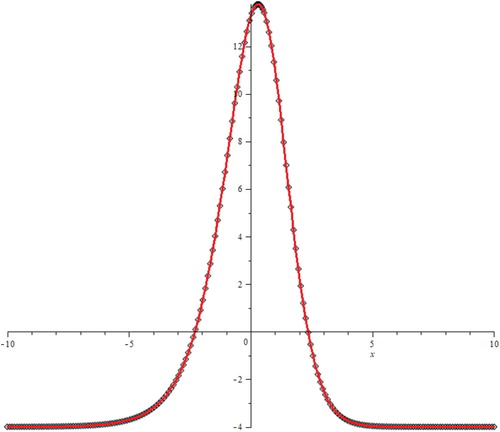
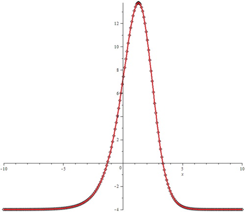
Figure 2. Exact solutions (ES) and approximate solutions (AS) of Example 4.2 for t=1.0 and different values of x.

5. Conclusions

In this work, we applied the reproducing kernel Hilbert space method to the generalized Kuramoto–Sivashinsky equation. We tested the power of the method on two numerical experiments. We demonstrated our results via tables. We used very important reproducing kernel functions to get the desired results. We concluded that the proposed technique can be applied to more complicated problems.

Disclosure statement

No potential conflict of interest was reported by the authors.

ORCID

Ebenezer Bonyah  http://orcid.org/0000-0003-0808-4504

References

- Khater AH, Temsah RS. Numerical solutions of the generalized Kuramoto–Sivashinsky equation by Chebyshev spectral collocation methods. Comput Math Appl. 2008;56: 1465–1472.
- Kuramoto Y, Tsuzuki T. Persistent propagation of concentration waves in dissipative media far from thermal equilibrium. Prog Theor Phys. 1976;55: 356–369.
- Lakestani M, Dehghan M. Numerical solutions of the generalized Kuramoto–Sivashinsky equation using B-spline functions. Appl Math Model. 2012;36: 605–617.
- Hooper AP, Grimshaw R. Nonlinear instability at the interface between two viscous fluids. Phys Fluids. 1985;28: 37–45.
- Sivashinsky GI. Instabilities, pattern-formation, and turbulence in flames. Ann Rev Fluid Mech. 1983;15:179–199.
- Demekhin Saprykin S, Kalliadasis EA. Two-dimensional wave dynamics in thin films, I. Stationary solitary pulses. J Phys Fluids. 2005;17: 1–16.
- Grimshaw R, Hooper AP. The non-existence of a certain class of travelling wave solutions of the Kuramoto–Sivashinsky equation. Phys D. 1991;50: 231–238.
- Liu X. Gevrey class regularity and approximate inertial manifolds for the Kuramoto–Sivashinsky equation. Phys D. 1991;50: 135–151.
- Lai H, Ma CF. Lattice Boltzmann method for the generalized Kuramoto–Sivashinsky equation. Phys A. 2009;388: 1405–1412.
- Dehghan M, Shokri A. A numerical method for solution of the two-dimensional sine-Gordon equation using the radial basis functions. Math Comput Simul. 2008;79: 700–715.
- Tatari M, Dehghan M. On the solution of the non-local parabolic partial differential equations via radial basis functions. Appl Math Model. 2009;33: 1729–1738.
- Uddin M, Haq S, Islam S. A mesh-free numerical method for solution of the family of Kuramoto–Sivashinsky equations. Appl Math Comput. 2009;212: 458–469.
- Xu Y, Shu CW. Local discontinuous Galerkin methods for the Kuramoto–Sivashinsky equations and the Ito-type coupled KdV equations. Comput Methods Appl Mech Eng. 2006;195: 3430–3447.
- Fan E. Extended tanh-function method and its applications to nonlinear equations. Phys Lett A. 2000;277: 212–218.
- Zaremba S. L'équation biharmonique et une classe remarquable de fonctions fondamentales harmoniques. Bull Int Acad Sci Cracovie 1907;147–196.
- Zaremba S. Sur le calcul numérique des fonctions demandées dan le probléme de dirichlet et le probleme hydrodynamique. Bull Int Acad Sci Cracovie 1908; 125–195.
- Geng F. A new reproducing kernel Hilbert space method for solving nonlinear fourth-order boundary value problems. Appl Math Model. 2009;213: 163–169.
- Zhang S, Liu L, Diao L. Reproducing kernel functions represented by form of polynomials. In: Proceedings of the Second Symposium International Computer Science and Computational Technology, Vol. 26; 2009. p. 353–358.
- Gumah G, Moaddy K, Al-Smadi M, et al. Solutions of uncertain Volterra integral equations by fitted reproducing kernel Hilbert space method. J Funct Spaces 2016; Article ID 2920463.
- Saadeh R, Al-Smadi M, Gumah G, et al. Numerical investigation for solving two-point fuzzy boundary value problems by reproducing kernel approach. Appl Math Inf Sci. 2016;10(6): 1–13.
- Arqub OA, Al-Smadi M, Momani S, et al. Numerical solutions of fuzzy differential equations using reproducing kernel Hilbert space method. Soft Comput. 2016;20: 3283–3302.
- Hashemi MS, Akgül A., Inc M, et al. Solving the Lane–Emden equation within a reproducing kernel method and group preserving scheme. Mathematics. 2017;5(4): 77.
- Arqub OA, Al-Smadi M, Momani S, et al. Numerical solutions of fractional differential equations of Lane–Emden type by an accurate technique. Adv Differ Equ. 2015;2015: 220.
- Inc M, Akgül A. The reproducing kernel Hilbert space method for solving Troesch's problem. J Assoc Arab Univ Basic Appl Sci. 2013;14: 19–27.
- Inc M, Akgül A. Approximate solutions for MHD squeezing fluid flow by a novel method. Bound Value Probl. 2014;2014: 18.
- Inc M, Akgül A, Geng F. Reproducing kernel Hilbert space method for solving Bratu's problem. Bull Malays Math Soc. 2015;38: 271–287.
- Inc M, Akgül A, Kilicman A. Numerical solutions of the second order one-dimensional telegraph equation based on reproducing kernel Hilbert space method. Abstr Appl Anal. 2013;2013: 13.
- Inc M, Akgül A, Kilicman A. On solving KdV equation using reproducing kernel Hilbert space method. Abstr Appl Anal 2013; Article ID 578942, 11 pages.
- Cui M, Lin Y. Nonlinear numerical analysis in the reproducing kernel space. New York: Nova Science Publishers Inc.; 2009.
- Arqub OA, Al-Smadi M. Atangana-Baleanu fractional approach to the solutions of Bagley-Torvik and Painlevé equations in Hilbert space. Chaos Solitons Fractals. 2018;117: 161–167.
- Arqub OA, Maayah B. Numerical solutions of integrodifferential equations of Fredholm operator type in the sense of the Atangana-Baleanu fractional operator. Chaos Solitons Fractals. 2018;117: 117–124.
- Arqub OA, Al-Smadi M. Numerical algorithm for solving time-fractional partial integrodifferential equations subject to initial and Dirichlet boundary conditions. Numer Methods Partial Differ Equ. 2018;34: 1577–1597.
- Arqub OA. Solutions of time-fractional Tricomi and Keldysh equations of Dirichlet functions types in Hilbert space. Numer Methods Partial Differ Equ. 2018;34: 1759–1780.
- Arqub OA. Application of residual power series method for the solution of time-fractional Schrodinger equations in one-dimensional space. Fundam Inform. 2019;166: 87–110.
- Arqub OA. Numerical algorithm for the solutions of fractional order systems of Dirichlet function types with comparative analysis. Fundam Inform. 2019;166: 111–137.
- Arqub OA. Numerical solutions of systems of first-order, two-point BVPs based on the reproducing kernel algorithm. Calcolo. 2018;55: 1–28.
- Arqub OA. Fitted reproducing kernel Hilbert space method for the solutions of some certain classes of time-fractional partial differential equations subject to initial and Neumann boundary conditions. Comput Math Appl. 2017;73: 1243–1261.
- Alvandia A, Paripourb M. Reproducing kernel method for a class of weakly singular Fredholm integral equations. J Taibah Univ Sci. 2018;12(4): 409–414.
- Khan H, Arif M, Mohyud-Dinb ST, et al. Numerical solutions to systems of fractional Voltera Integro differential equations, using Chebyshev wavelet method. J Taibah Univ Sci. 2018;12(5): 584–591.
- Hesameddini E, Shahbaz M. A reliable algorithm based on the shifted orthonormal Bernstein polynomials for solving Volterra–Fredholm integral equations. J Taibah Univ Sci. 2018;12(4): 427–438.
- Yousif MA, Manaa SA, Easif FH. Solving the Kuramoto–Sivashinsky equation via variational iteration method. Int J Appl Math Res. 2014;3(3): 260–264.