Effect of variation of charge in the circular restricted three-body problem with variable masses

Abstract

In the present paper, we are concerned by some investigation on circular restricted three-body problem (CR3BP), where we assume that the primaries have variable masses and variable charges. Among the principal tools used in the present study, we cite the well known Meshcherskii transformation. We have derived the equations of motion and Jacobi integral which differ by variation constant k and charge q from the classical restricted three-body problem. More exactly, in this paper, we have drawn the equilibrium points, the zero-velocity curves, the periodic orbits, the surfaces and the basins of attraction for the different values of charge. We have found one equilibrium point when the charge is q=0.4 and three equilibrium points when its value is q=0.501. We also have drawn the periodic orbits for these two values of charge and found that they are periodic. We have also plotted the zero-velocity surfaces for these two values of charges and found a tremendous variation in these two surfaces. We notice that the Poincaré surfaces of section are shifting away from the origin, when we increase the value of charge. We also got different surfaces for the motion of infinitesimal body, with respect to the variations of charge. The basins of attraction have been drawn for these two values of charge by using Newton-Raphson iterative method. We also noticed that by increasing the values of charge, the basins of attraction are shrinking. For the stability of the equilibrium points that we have studied, we found that, among them, one is stable and three others are unstable.

Keywords:

• Jacobi integral
• equilibrium points
• periodic orbits
• poincaré surface
• three-body problem
• meshcherskii transformation
• basins of attraction
• zero-velocity curves

2010 MSC:

• 70F07
• 70F15

1. Introduction

Many scientists have been extremely concerned by the study of the restricted three-body problem with diverse perturbations like, forms of the bodies, radiation pressure, variable mass, Pointing-Robertson drag, albedo, charged body, magnetic dipole, resonance and so on.

Before the studies of the three-body problem, Jeans in [1] has been concerned by the study of the two-body problem with variable mass and then Meshcherskii [2, 3] made some investigations on the mechanics of the bodies with variable mass. Recently, Shrivastava et al. [4] determined the equations relating to the movement in the restricted three-body problem with decreasing masses with respect to the time. In his investigation, he used the Jeans' law and Meshcherskii transformation. Dionysiou et al. [5, 6] have been concerned by the stability of the equilibrium points in the circular restricted charged three-body problem. Simultaneously, Lukyanov [7] elaborates a study on the particular solution of the restricted problem of three bodies with variable mass by using Meshcherskii transformation. On the other hand, Singh et al. in a series of papers, [8–11] explored the restricted three-body problem with different perturbations. Zhang et al. [12] investigated the photogravitational restricted three-body problem, with the assumption that the infinitesimal body has a variable mass according to Jeans' law. They observed that the displacement around the triangular equilibrium points is not stable. More recently, Bengochea et al. [13] investigated the location and the stability of the equilibrium points of the circular restricted charged three-body problem in a plane. Abouelmagd et al. [14] studied the location of the out of plane, equilibrium points in the special case of a non-isotropic variation of the mass in the restricted three-body problem. As a contribution to the subject, Ansari [15] made a numerical investigation to study the equilibrium points, the zero-velocity curves, the time series and the Poincaré surface of section for the circular restricted three-body problem. He considered a system, where one of the primaries has an oblate spheroid form, the second represents the source of radiation pressure and all the components of the system have variable masses in time. Moreover, he found that all the equilibrium points are unstable. An analogous study has been done in Ansari et al. [16], where the primaries are supposed to be straight segments. Alhussain in [17] has studied the effects of Poynting-Robertson drag on the circular restricted three-body problem with variable masses. In counter part, the four-body problem has been the subject of investigation made in Ansari et al. [18]. More exactly, the authors studied the circular restricted four-body problem with variable masses subjected to the effect of some perturbations. They have been concerned by the nature of the equilibrium points, the zero-velocity curves, the time series and the Poincaré surface of section.

On the other hand, the basins of attraction in the restricted n-body problem have been an attractive subject for many other researchers. We can cite, for example, Douskos [19], Kumari [20], Asique [21], Zotos [22, 23], etc

In this paper, we have investigated, using Meshcherskii transformation, the circular restricted three-body problem, where the primaries are supposed to have variable masses and variable charges. The sections of the paper are as follows.

In the introduction section, we have gave a short overview on the principal works made on the subject. In the equations of motion section, we have derived the equations of motion and the Jacobi integral. In the numerical calculation section, we have drawn the equilibrium points, the zero-velocity curves, the periodic orbits, the surfaces for the different values of charge and the basins of attraction. In the section devoted to the stability, we have examined the stability of the equilibrium points and finally, We have summarized our work in a the conclusion section. As a first opinion, we think that the treated problem can have a certain number of applications in the astrophysics. We can apply this study to a system constitutes by three stars. We know that, due to the radiation that they emit, stars have a variable mass and variable charge.

2. Equations of motion

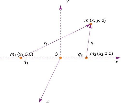
Assume $m_1\left(t\right)$ and $m_2\left(t\right)$ be the masses of two bodies having respectively, $q_1\left(t\right)$ and $q_2\left(t\right)$ as charges. We assume that all the introduced parameters are time variable and these bodies are revolving in a circular orbits around their common center of mass which is considered as origin and placed either sides of the origin O on the x-axis. The line orthogonal to the x-axis and passing through the origin is taken as y-axis. On the other hand, the line passing through the origin and orthogonal to the plane of motion of the primaries is considered as z-axis. Our investigation will be made with respect to the synodic coordinate system which coincides with the inertial coordinate system at the time t=0 and rotating with an angular velocity ω with respect to the z-axis (Figure 1). To the previous system, we add a third charged body with a constant mass m that will be called the infinitesimal body in the sequel. We suppose that this infinitesimal body will be subject to the actions (attracted or repulsed) of the primaries but does not have any influence on their behavior or motion. The total force per unit of charge exerted on the infinitesimal body will be as follows: (1) $\begin{array}{rl}\overrightarrow{F}& =\overrightarrow{F_1}+\overrightarrow{F_2}\\ & =-\frac{m(G{m}_1-K_e{q}_1)\overrightarrow{r_1}}{r_1^3}-\frac{m(G{m}_2-K_e{q}_2)\overrightarrow{r_2}}{r_2^3}\end{array}$(1) where $F_i$ are the forces exerted by the respective primaries on the infinitesimal body.

Figure 1. Geometric configuration of the problem.

Using the procedure given by Dionysiou [5], we can write the equations of motion of the infinitesimal body in the vector form under the influence of the variable mass and charges of the primaries as follows: (2) $m(\ddot{\overrightarrow{r}}+2\overrightarrow{\omega }\times \dot{\overrightarrow{r}}+\dot{\overrightarrow{\omega }}\times \overrightarrow{r}+\overrightarrow{\omega }\times (\overrightarrow{\omega }\times \overrightarrow{r}\left)\right)=\overrightarrow{F},$(2) where, $\ddot{\overrightarrow{r}}$ is the relative acceleration, $2\overrightarrow{\omega }\times \dot{\phantom{a}}\overrightarrow{r}$ is the coriolis acceleration, $\dot{\overrightarrow{\omega }}\times \overrightarrow{r}$ is the Euler acceleration, $\overrightarrow{\omega }\times (\overrightarrow{\omega }\times \overrightarrow{r})$ is the centrifugal acceleration and $\overrightarrow{r}$ is the position vector of the infinitesimal body and $\overrightarrow{\omega }$ is the velocity vector.

Comparing x,y,z components of both sides of Equation (2(2) $m(\ddot{\overrightarrow{r}}+2\overrightarrow{\omega }\times \dot{\overrightarrow{r}}+\dot{\overrightarrow{\omega }}\times \overrightarrow{r}+\overrightarrow{\omega }\times (\overrightarrow{\omega }\times \overrightarrow{r}\left)\right)=\overrightarrow{F},$(2) ), we get (3) $\begin{array}{rl}\ddot{x}-2\omega \dot{y}-\dot{\omega }y-{\omega }^{2}x& =-\frac{({\mu }_1-p_1)(x-x_1)}{r_1^3}\\ & -\frac{({\mu }_2-p_2)(x-x_2)}{r_2^3},\\ \ddot{y}+2\omega \dot{x}+\dot{\omega }x-{\omega }^{2}y& =-\frac{({\mu }_1-p_1)y}{r_1^3}-\frac{({\mu }_2-p_2)y}{r_2^3},\\ \ddot{z}& =-\frac{({\mu }_1-p_1)z}{r_1^3}-\frac{({\mu }_2-p_2)z}{r_2^3}.\end{array}$(3) where, $r_i^2=(x-x_i{)}^2+y^2+z^2,(i=1,2),$ are the distance from the primaries to the infinitesimal body, ${\mu }_i=G{m}_i,p_i=K_e{q}_i,(i=1,2),$ are the masses and charges of the primaries, G and $K_e$ are the gravitational constant and Coulomb's constant, respectively.

By the following Meshcherskii transformation $\begin{array}{rl}x& =\xi R\left(t\right),y=\eta R\left(t\right),z=\zeta R\left(t\right),\\ \frac{\mathrm{d}t}{\mathrm{d}\tau }& =R^2\left(t\right),\omega \left(t\right)=\frac{{\omega }_0}{R^2\left(t\right)},\\ r_i& ={\rho }_{i}R\left(t\right),x_i={\xi }_{i}R\left(t\right),\\ \mu \left(t\right)& ={\mu }_1\left(t\right)+{\mu }_2\left(t\right)=\frac{{\mu }_0}{R\left(t\right)},\\ p\left(t\right)& =p_1\left(t\right)+p_2\left(t\right)=\frac{p_0}{R\left(t\right)},\\ {\mu }_i\left(t\right)& =\frac{{\mu }_{i0}}{R\left(t\right)},p_i\left(t\right)=\frac{p_{i0}}{R\left(t\right)},(i=1,2),\\ R\left(t\right)& =\sqrt{a{t}^2+2bt+c},\end{array}$ where $a,b,c,{\mu }_0,{\mu }_{10},{\mu }_{20},p_{10},p_{20},m_0$ are constants, the equation of motion (3(3) $\begin{array}{rl}\ddot{x}-2\omega \dot{y}-\dot{\omega }y-{\omega }^{2}x& =-\frac{({\mu }_1-p_1)(x-x_1)}{r_1^3}\\ & -\frac{({\mu }_2-p_2)(x-x_2)}{r_2^3},\\ \ddot{y}+2\omega \dot{x}+\dot{\omega }x-{\omega }^{2}y& =-\frac{({\mu }_1-p_1)y}{r_1^3}-\frac{({\mu }_2-p_2)y}{r_2^3},\\ \ddot{z}& =-\frac{({\mu }_1-p_1)z}{r_1^3}-\frac{({\mu }_2-p_2)z}{r_2^3}.\end{array}$(3) ) becomes (4) $\begin{array}{rl}{\xi }^{″}-2{\omega }_0{\eta }^{\prime }& =\frac{\mathrm{\partial }\mathrm{\Omega }}{\mathrm{\partial }\xi },\\ {\eta }^{″}+2{\omega }_0{\xi }^{\prime }& =\frac{\mathrm{\partial }\mathrm{\Omega }}{\mathrm{\partial }\eta },\\ {\zeta }^{″}& =\frac{\mathrm{\partial }\mathrm{\Omega }}{\mathrm{\partial }\zeta }.\end{array}$(4) where, $\begin{array}{rl}\mathrm{\Omega }& =\frac{{\omega }_0^2}{2}({\xi }^2+{\eta }^2)-\frac{(ac-b^2)}{2}({\xi }^2+{\eta }^2+{\zeta }^2)\\ & +\frac{({\mu }_{10}-p_{10})}{{\rho }_1}+\frac{({\mu }_{20}-p_{20})}{{\rho }_2},\\ {\rho }_i^2& =(\xi -{\xi }_i{)}^2+{\eta }^2+{\zeta }^2,{\xi }_1=\frac{-{\mu }_{20}}{{\mu }_0}{\rho }_{12},{\xi }_2=\frac{{\mu }_{10}}{{\mu }_0}{\rho }_{12},\end{array}$ Prime (') is the derivative w.r.to τ and ${\rho }_{12}$ is the distance between the primaries.

We choose units of mass, distance, charge and time such that $\begin{array}{rl}& {\mu }_0=1,{\rho }_{12}=1,G=1,\\ & K_e=1,p_0=1,{\omega }_0=1\end{array}$ and introduce the mass and charge parameters υ and q as follows $\frac{{\mu }_{10}}{{\mu }_0}=1-\upsilon ,\frac{{\mu }_{20}}{{\mu }_0}=\upsilon ,\frac{p_{10}}{p_0}=1-q,\frac{p_{20}}{p_0}=q,$ where, υ is the ratio of the mass of the primaries with respect to the total mass of the primaries and q is the ratio of the charge of the primaries with respect to the total charge of the primaries.

Finally, the equations of motion (4(4) $\begin{array}{rl}{\xi }^{″}-2{\omega }_0{\eta }^{\prime }& =\frac{\mathrm{\partial }\mathrm{\Omega }}{\mathrm{\partial }\xi },\\ {\eta }^{″}+2{\omega }_0{\xi }^{\prime }& =\frac{\mathrm{\partial }\mathrm{\Omega }}{\mathrm{\partial }\eta },\\ {\zeta }^{″}& =\frac{\mathrm{\partial }\mathrm{\Omega }}{\mathrm{\partial }\zeta }.\end{array}$(4) ) become (5) $\begin{array}{rl}{\xi }^{″}-2{\eta }^{\prime }& =\frac{\mathrm{\partial }V}{\mathrm{\partial }\xi },\\ {\eta }^{″}+2{\xi }^{\prime }& =\frac{\mathrm{\partial }V}{\mathrm{\partial }\eta },\\ {\zeta }^{″}& =\frac{\mathrm{\partial }V}{\mathrm{\partial }\zeta },\end{array}$(5) where, $\begin{array}{rl}V& =\frac{k}{2}({\xi }^2+{\eta }^2)-\frac{(1-k)}{2}{\zeta }^2+\frac{(q-\upsilon )}{{\rho }_1}+\frac{(\upsilon -q)}{{\rho }_2},\\ {\rho }_i^2& =(\xi -{\xi }_i{)}^2+{\eta }^2+{\zeta }^2,{\xi }_1=-\upsilon ,\\ {\xi }_2& =1-\upsilon ,1-k=ac-b^2.\end{array}$ From the equations of motion (5(5) $\begin{array}{rl}{\xi }^{″}-2{\eta }^{\prime }& =\frac{\mathrm{\partial }V}{\mathrm{\partial }\xi },\\ {\eta }^{″}+2{\xi }^{\prime }& =\frac{\mathrm{\partial }V}{\mathrm{\partial }\eta },\\ {\zeta }^{″}& =\frac{\mathrm{\partial }V}{\mathrm{\partial }\zeta },\end{array}$(5) ), we can derive the Jacobi integral as follows (6) $J(\xi ,\eta ,\zeta ,{\xi }^{\prime },{\eta }^{\prime },{\zeta }^{\prime })=({\xi }^{\prime 2}+{\eta }^{\prime 2}+{\zeta }^{\prime 2})=2V-C,$(6) where constant C is the well-known Jacobi Integral constant.

3. Numerical calculations

In this section, we use Mathematica software to give an overview of the locations of the equilibrium points, zero-velocity curves, periodic orbits, surfaces and the basins of attraction through graphs.

3.1. Locations of equilibrium points

The locations of the equilibrium points can be determined by setting in (5(5) $\begin{array}{rl}{\xi }^{″}-2{\eta }^{\prime }& =\frac{\mathrm{\partial }V}{\mathrm{\partial }\xi },\\ {\eta }^{″}+2{\xi }^{\prime }& =\frac{\mathrm{\partial }V}{\mathrm{\partial }\eta },\\ {\zeta }^{″}& =\frac{\mathrm{\partial }V}{\mathrm{\partial }\zeta },\end{array}$(5) ), the followings ${\xi }^{″}={\eta }^{″}={\zeta }^{″}={\xi }^{\prime }={\eta }^{\prime }={\zeta }^{\prime }=0$, we then obtain.

$V_{\xi }=0,V_{\eta }=0,V_{\zeta }=0.$ More exactly, these relations mean that (7) $\begin{array}{rl}k\xi -\frac{(q-\upsilon )(\xi +\upsilon )}{{\rho }_1^3}-\frac{(\upsilon -q)(\xi +\upsilon -1)}{{\rho }_2^3}& =0,\end{array}$(7) (8) $\begin{array}{rl}k\eta -\frac{(q-\upsilon )\eta }{{\rho }_1^3}-\frac{(\upsilon -q)\eta }{{\rho }_2^3}& =0,\end{array}$(8) (9) $\begin{array}{rl}(k-1)\zeta -\frac{(q-\upsilon )\zeta }{{\rho }_1^3}-\frac{(\upsilon -q)\zeta }{{\rho }_2^3}& =0.\end{array}$(9)

The real solutions of (7(7) $\begin{array}{rl}k\xi -\frac{(q-\upsilon )(\xi +\upsilon )}{{\rho }_1^3}-\frac{(\upsilon -q)(\xi +\upsilon -1)}{{\rho }_2^3}& =0,\end{array}$(7) ), (8(8) $\begin{array}{rl}k\eta -\frac{(q-\upsilon )\eta }{{\rho }_1^3}-\frac{(\upsilon -q)\eta }{{\rho }_2^3}& =0,\end{array}$(8) ) and (9(9) $\begin{array}{rl}(k-1)\zeta -\frac{(q-\upsilon )\zeta }{{\rho }_1^3}-\frac{(\upsilon -q)\zeta }{{\rho }_2^3}& =0.\end{array}$(9) ) are called the “Equilibrium points” or the “Lagrangian points”. Obviously, from the (8(8) $\begin{array}{rl}k\eta -\frac{(q-\upsilon )\eta }{{\rho }_1^3}-\frac{(\upsilon -q)\eta }{{\rho }_2^3}& =0,\end{array}$(8) ) and (9(9) $\begin{array}{rl}(k-1)\zeta -\frac{(q-\upsilon )\zeta }{{\rho }_1^3}-\frac{(\upsilon -q)\zeta }{{\rho }_2^3}& =0.\end{array}$(9) ), we deduce that $\eta =\zeta =0$ and then all the equilibrium points are located on the $x-$axis, (i.e. only collinear equilibrium points exist). Here we have shown the locations of equilibrium points for the different values of the charge.

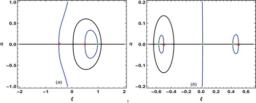
For q=0.4, we get one equilibrium point (the green point in Figure 2(a)) and for q=0.501, we get three equilibrium points (the points in green color of Figure 2(b)). Finally, in all these figures, the red color points indicate the locations of primaries.

Figure 2. Locations of equilibrium points for q=0.4 (a) and for q=0.501 (b). The green points indicate the equilibrium points and red points indicate the locations of the primaries.

3.2. Zero-velocity curves

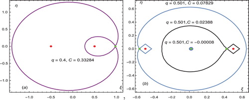
For the zero velocity curves, if we set ${\xi }^{\prime }={\eta }^{\prime }={\zeta }^{\prime }=0$ in (6(6) $J(\xi ,\eta ,\zeta ,{\xi }^{\prime },{\eta }^{\prime },{\zeta }^{\prime })=({\xi }^{\prime 2}+{\eta }^{\prime 2}+{\zeta }^{\prime 2})=2V-C,$(6) ) (i.e. 2V −C=0), we get the figures (Figure 3(a,b)). In the first figure, we get one curve (purple) for q=0.4,C=0.33284, since there is only one equilibrium point (see Figure 2(a)). In the second, we get three curves for $q=0.501,C=0.07829$ (Magneta curve), $q=0.501,C=0.02388$ (Black curve) and for $q=0.501,C=-0.00008$ (Blue curve). In Figure 3(a,b), the green points indicate the locations of the equilibrium points and the red points indicate the locations of the primaries.

Figure 3. Zero-velocity curves $\left(a\right)$ for $q=0.4$ and $\left(b\right)$ for q=0.501.

3.3. Periodic orbits

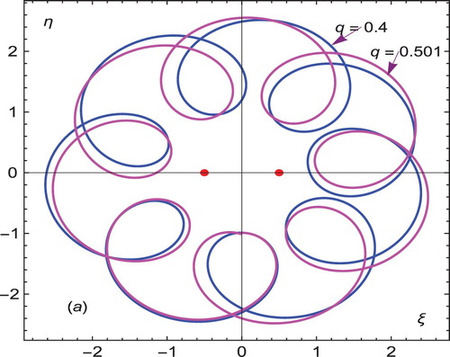
We have found an epitrochoid periodic orbits (Figure 4) for the different values of the charge. In this figure, blue color curve correspond to q=0.4 and magenta color curve is obtained for q=0.501. In this situation, the curves are shifting by some phase angles.

Figure 4. Epitrochoid periodic orbits for the variations of charge.

4. Surfaces

The present section is devoted to the different surfaces obtained for the different values of the charge.

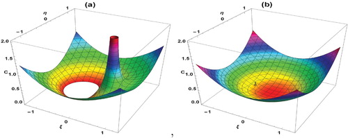
4.1. Zero-velocity surface

Figure 5(a) corresponds to the zero-velocity surfaces for $q=0.4$ and Figure 5(b) corresponds to the zero-velocity surfaces for q=0.501. These surfaces are obtained from Equation (6(6) $J(\xi ,\eta ,\zeta ,{\xi }^{\prime },{\eta }^{\prime },{\zeta }^{\prime })=({\xi }^{\prime 2}+{\eta }^{\prime 2}+{\zeta }^{\prime 2})=2V-C,$(6) ) using the Mathematica software.

Figure 5. Zero-velocity surfaces $\left(a\right)$ for $q=0.4$ and $\left(b\right)$ for q=0.501.

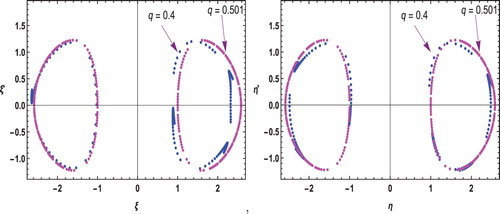
4.2. Poincaré surface of section

In this subsection, we have drawn the Poincaré surface. In Figures 6, the blue color surface is obtained for q=0.4 and the magenta color one is obtained for q=0.501.

Figure 6. (a):Poincaré surfaces of section in $\xi -{\xi }^{\prime }$ plane. (b):Poincaré surfaces of section in $\eta -{\eta }^{\prime }$ plane.

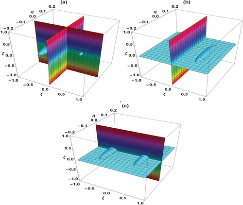
4.3. Surfaces of the motion of the infinitesimal body

The surfaces of the motion of the infinitesimal body for q=0.4 (Figure 7( a–c)) and for q=0.501 (Figure 8( a–c)) are obtained from Equations (7(7) $\begin{array}{rl}k\xi -\frac{(q-\upsilon )(\xi +\upsilon )}{{\rho }_1^3}-\frac{(\upsilon -q)(\xi +\upsilon -1)}{{\rho }_2^3}& =0,\end{array}$(7) ) –( 9(9) $\begin{array}{rl}(k-1)\zeta -\frac{(q-\upsilon )\zeta }{{\rho }_1^3}-\frac{(\upsilon -q)\zeta }{{\rho }_2^3}& =0.\end{array}$(9) ) using Mathematica Software.

Figure 7. The surfaces of the motion of the infinitesimal body for $q=0.4$.

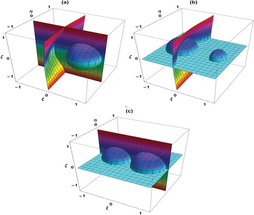
Figure 8. The surfaces of the motion of the infinitesimal body for q=0.501.

5. Basins of attraction

By using the Newton-Raphson iterative method, it is easy to draw the the basins of attraction with respect to the variation of the charge. The iterative algorithm used to reach this goal is given by the following system. (10) $\begin{array}{rl}& {\xi }_{n+1}={\xi }_n-{\left(\frac{V_{\xi }{V}_{\eta \eta }-V_{\eta }{V}_{\xi \eta }}{V_{\xi \xi }{V}_{\eta \eta }-V_{\xi \eta V_{\eta \xi }}}\right)}_{({\xi }_n,{\eta }_n)},\\ & {\eta }_{n+1}={\eta }_n-(\frac{V_{\eta }{V}_{\xi \xi }-V_{\xi }{V}_{\eta \xi }}{V_{\xi \xi }{V}_{\eta \eta }-V_{\xi \eta V_{\eta \xi }}}{)}_{({\xi }_n,{\eta }_n)}.\end{array}$(10) where ${\xi }_n,{\eta }_n$ are the values of the ξ and η coordinates of the nth step of the Newton-Raphson iterative process. The initial point $(\xi ,\eta )$ is inside the basin of attraction of the attractor if this point converges rapidly to one of the equilibrium points. This process stops when the successive approximation converges to an attractor, with some predefined accuracy. For the classification of the equilibrium points on the $(\xi ,\eta )$ plane, we will use color code. In this way, a complete view of the basin structures created by the attractors (see Figures 9 and 10).

Figure 9. (a) Basins of attraction at q=0.4. (b) Zoomed part of Figure 9(a) near primaries.

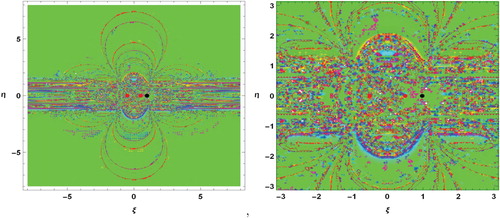
Figure 10. (a) Basins of attraction at q=0.501. (b) Zoomed part of Figure 10(a) near primaries.

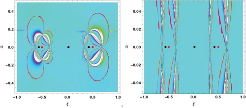
Details of the locations of the equilibrium points and the primaries can be seen in Figures 9(b) and  10(b), respectively. In these figures, black points denote locations of the equilibrium points and red points denote the primaries.

6. Stability

To examine the stability of the equilibrium points, we use the procedure given by Mccuskey [24].

If we substitute $\xi ={\xi }_0+a,\eta ={\eta }_0+b$ and $\zeta ={\zeta }_0+c$ in Equation (5(5) $\begin{array}{rl}{\xi }^{″}-2{\eta }^{\prime }& =\frac{\mathrm{\partial }V}{\mathrm{\partial }\xi },\\ {\eta }^{″}+2{\xi }^{\prime }& =\frac{\mathrm{\partial }V}{\mathrm{\partial }\eta },\\ {\zeta }^{″}& =\frac{\mathrm{\partial }V}{\mathrm{\partial }\zeta },\end{array}$(5) ), we get; (11) $\begin{array}{rl}{a}^{″}-2b^{\prime }& =a{V}_{\xi \xi }^0+b{V}_{\xi \eta }^0+c{V}_{\xi \zeta }^0\\ b^{″}+2a^{\prime }& =a{V}_{\eta \xi }^0+b{V}_{\eta \eta }^0+c{V}_{\eta \zeta }^0\\ c^{″}& =a{V}_{\zeta \xi }^0+b{V}_{\zeta \eta }^0+c{V}_{\zeta \zeta }^0\end{array}$(11) where a,b and c are small displacements of the infinitesimal body from the equilibrium point and the superscript zero denotes the value at the equilibrium point.

To solve Equation (11(11) $\begin{array}{rl}{a}^{″}-2b^{\prime }& =a{V}_{\xi \xi }^0+b{V}_{\xi \eta }^0+c{V}_{\xi \zeta }^0\\ b^{″}+2a^{\prime }& =a{V}_{\eta \xi }^0+b{V}_{\eta \eta }^0+c{V}_{\eta \zeta }^0\\ c^{″}& =a{V}_{\zeta \xi }^0+b{V}_{\zeta \eta }^0+c{V}_{\zeta \zeta }^0\end{array}$(11) ), let us set $a=\alpha e^{\lambda \tau },b=\beta e^{\lambda \tau },c=\gamma e^{\lambda \tau }$ where $\alpha ,\beta$ and γ are some parameters.

By substituting the previous values in Equation (11(11) $\begin{array}{rl}{a}^{″}-2b^{\prime }& =a{V}_{\xi \xi }^0+b{V}_{\xi \eta }^0+c{V}_{\xi \zeta }^0\\ b^{″}+2a^{\prime }& =a{V}_{\eta \xi }^0+b{V}_{\eta \eta }^0+c{V}_{\eta \zeta }^0\\ c^{″}& =a{V}_{\zeta \xi }^0+b{V}_{\zeta \eta }^0+c{V}_{\zeta \zeta }^0\end{array}$(11) ) and rearranging if necessary, we get (12) $\begin{array}{rl}\alpha ({\lambda }^2-V_{\xi \xi }^0)-\beta (2\lambda +V_{\xi \eta }^0)-\gamma V_{\xi \zeta }^0& =0\\ \alpha (2\lambda -V_{\eta \xi }^0)+\beta ({\lambda }^2-V_{\eta \eta }^0)-\gamma V_{\eta \zeta }^0& =0\\ -\alpha V_{\zeta \xi }^0-\beta V_{\zeta \eta }^0+\gamma ({\lambda }^2-V_{\zeta \zeta }^0)& =0.\end{array}$(12) The system (12(12) $\begin{array}{rl}\alpha ({\lambda }^2-V_{\xi \xi }^0)-\beta (2\lambda +V_{\xi \eta }^0)-\gamma V_{\xi \zeta }^0& =0\\ \alpha (2\lambda -V_{\eta \xi }^0)+\beta ({\lambda }^2-V_{\eta \eta }^0)-\gamma V_{\eta \zeta }^0& =0\\ -\alpha V_{\zeta \xi }^0-\beta V_{\zeta \eta }^0+\gamma ({\lambda }^2-V_{\zeta \zeta }^0)& =0.\end{array}$(12) ) will have a non-trivial solution for any $\alpha ,\beta$ and γ if $\left|\begin{array}{ccc}{\lambda }^2-V_{\xi \xi }^0& -2\lambda -V_{\xi \eta }^0& -V_{\xi \zeta }^0\\ \\ 2\lambda -V_{\eta \xi }^0& {\lambda }^2-V_{\eta \eta }^0& -V_{\eta \zeta }^0\\ \\ -V_{\zeta \xi }^0& -V_{\zeta \eta }^0& {\lambda }^2-V_{\zeta \zeta }^0\end{array}\right|=0$ and the above determinant is equal to (13) $\begin{array}{rl}& {\lambda }^6+{\lambda }^4(4-V_{\xi \xi }^0-V_{\eta \eta }^0-V_{\zeta \zeta }^0)+{\lambda }^2(-(V_{\xi \eta }^0{)}^2-(V_{\xi \zeta }^0{)}^2\\ & -(V_{\eta \zeta }^0{)}^2-4V_{\zeta \zeta }^0+V_{\xi \xi }^0{V}_{\eta \eta }^0+V_{\xi \xi }^0{V}_{\zeta \zeta }^0+V_{\eta \eta }^0{V}_{\zeta \zeta }^0)\\ & +\left(\right(V_{\xi \zeta }^0{)}^2{V}_{\eta \eta }^0+V_{\xi \xi }^0(V_{\eta \zeta }^0{)}^2+(V_{\xi \eta }^0{)}^2{V}_{\zeta \zeta }^0\\ & -2V_{\xi \eta }^0{V}_{\xi \zeta }^0{V}_{\eta \zeta }^0-V_{\xi \xi }^0{V}_{\eta \eta }^0{V}_{\zeta \zeta }^0)=0.\end{array}$(13)

In view of the study of the stability of the equilibrium points, we determine numerically the roots of Equation (13(13) $\begin{array}{rl}& {\lambda }^6+{\lambda }^4(4-V_{\xi \xi }^0-V_{\eta \eta }^0-V_{\zeta \zeta }^0)+{\lambda }^2(-(V_{\xi \eta }^0{)}^2-(V_{\xi \zeta }^0{)}^2\\ & -(V_{\eta \zeta }^0{)}^2-4V_{\zeta \zeta }^0+V_{\xi \xi }^0{V}_{\eta \eta }^0+V_{\xi \xi }^0{V}_{\zeta \zeta }^0+V_{\eta \eta }^0{V}_{\zeta \zeta }^0)\\ & +\left(\right(V_{\xi \zeta }^0{)}^2{V}_{\eta \eta }^0+V_{\xi \xi }^0(V_{\eta \zeta }^0{)}^2+(V_{\xi \eta }^0{)}^2{V}_{\zeta \zeta }^0\\ & -2V_{\xi \eta }^0{V}_{\xi \zeta }^0{V}_{\eta \zeta }^0-V_{\xi \xi }^0{V}_{\eta \eta }^0{V}_{\zeta \zeta }^0)=0.\end{array}$(13) ). Table 1 gives the roots of Equation (13(13) $\begin{array}{rl}& {\lambda }^6+{\lambda }^4(4-V_{\xi \xi }^0-V_{\eta \eta }^0-V_{\zeta \zeta }^0)+{\lambda }^2(-(V_{\xi \eta }^0{)}^2-(V_{\xi \zeta }^0{)}^2\\ & -(V_{\eta \zeta }^0{)}^2-4V_{\zeta \zeta }^0+V_{\xi \xi }^0{V}_{\eta \eta }^0+V_{\xi \xi }^0{V}_{\zeta \zeta }^0+V_{\eta \eta }^0{V}_{\zeta \zeta }^0)\\ & +\left(\right(V_{\xi \zeta }^0{)}^2{V}_{\eta \eta }^0+V_{\xi \xi }^0(V_{\eta \zeta }^0{)}^2+(V_{\xi \eta }^0{)}^2{V}_{\zeta \zeta }^0\\ & -2V_{\xi \eta }^0{V}_{\xi \zeta }^0{V}_{\eta \zeta }^0-V_{\xi \xi }^0{V}_{\eta \eta }^0{V}_{\zeta \zeta }^0)=0.\end{array}$(13) ) for the different values of the equilibrium points.

Table 1. Characteristic roots corresponding to each equilibrium point.

q	$(\xi ,\eta )$	λ
0.4	(0.9783183434, 0)	−0.6218790796, −1.2177202932 I,
		$+1.2177202932$ I, −1.6443512025 I,
		$+1.6443512025$ I, 0.6218790796
0.501	(-0.5663132332, 0)	−2.1917008069, −2.0070941992 I,
		$+2.0070941992$ I, −2.1389542543 I,
		$+2.1389542543$ I, 2.1917008069
0.501	(0.4228395029, 0)	−1.2551930819, −1.2180170977,
		−2.6189836431 I, 2.6189836431 I,
		1.2180170977, 1.2551930819
0.501	(0.0200971969, 0)	−0.2247714567 I,0.2247714567 I,
		−0.7733435483 I, +0.7733435483 I,
		−1.7752232390 I, +1.7752232390 I

From Figure  11, we observed that there is only one bounded region near the star. This bounded region is the stable region.

Figure 11. Distribution of the stable region.

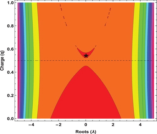
We notice that the point $(0.0200971969,0)$ is stable since it has purely imaginary roots. The other points are unstable since they have at least one positive real root.

7. Conclusion

In this paper, we have investigated the effect of the variation of charge in the circular restricted three-body problem with primaries having variable masses. This study has been done using Meshcherskii transformation. We have derived the equations of motion and Jacobi integral which differ by variation constant k and charge q from the classical restricted three-body problem. In the numerical calculation section, we have drawn the equilibrium points, the zero-velocity curves, the periodic orbits, the surfaces and the basins of attraction for the different values of charge. We have found one equilibrium point for $q=0.4$ and three equilibrium points for q=0.501. Relatively, to these four equilibrium points, we have plotted the zero-velocity curves where the infinitesimal body is supposed to easily move. We have also found the periodic orbits for these two values of charge and found that they are periodic. In the surfaces section, we have plotted the zero-velocity surfaces for these two values of charges and found a tremendous variation in these two surfaces. We have got that the Poincaré surfaces of section are shifting away from the origin by increasing the values of charge. In the motions of infinitesimal body, we have got different surfaces with respect to the variations of charges. We have drawn the basins of attraction for these two values of charges by using Newton-Raphson iterative method. We have noticed that by increasing the values of charge, the basins of attraction are shrinking. We have examined the stability of the equilibrium points and we have found that among the four equilibrium points, one is stable and three are unstable.

Disclosure statement

No potential conflict of interest was reported by the authors.

ORCID

Abdullah Abduljabar Ansari http://orcid.org/0000-0002-8361-810X

Rabah Kellil http://orcid.org/0000-0003-2582-3612

ZiyadAli Al-Hussain  http://orcid.org/0000-0001-8593-0239

Wasim Ul-Haq http://orcid.org/0000-0001-7148-1890

References

- Jeans JH. Astronomy and cosmogony. Cambridge: Cambridge University Press; 1928.
- Meshcherskii IV. Studies on the mechanics of bodies of variable mass. Moscow: GITTL; 1949.
- Meshcherskii IV. Works on the mechanics of bodies of variable mass. Moscow: GITT; 1952.
- Shrivastava AK, Ishwar B. Equations of motion of the restricted problem of three bodies with variable mass. Celest Mech. 1983;30:323–328. doi: 10.1007/BF01232197
- Dionysiou DD, Vaiopoulos DA. On the restricted circular three charged body problem. Astrophys Space Sci. 1987;135:253–260. doi: 10.1007/BF00641560
- Dionysiou DD, Stamou GG. Stability of the restricted circular and charged three-body problem. Astrophys Space Sci. 1989;152:1–8. doi: 10.1007/BF00645980
- Lukyanov LG. Particular solutions in the restricted problem of three bodies with variable mass. Astron Zh. 1989;66:180–187.
- Singh J. Effect of perturbations on the location of equilibrium points in the restricted problem of three bodies with variable mass. Celest Mech. 1984;32(4):297–305. doi: 10.1007/BF01229086
- Singh J, Ishwar B. Effect of perturbations on the stability of triangular points in the restricted problem of three bodies with variable mass. Celest Mech. 1985;35:201–207. doi: 10.1007/BF01227652
- Singh J, Leke O. Stability of photogravitational restricted three-body problem with variable mass. Astrophys Space Sci. 2010;326(2):305–314. doi: 10.1007/s10509-009-0253-x
- Singh J, Leke O. Existence and stability of equilibrium points in the robe's restricted three-body problem with variable masses. IJAA. 2013;3:113–122. doi:10.4236/ijaa.2013.32013.
- Zhang MJ, Zhao CY, Xiong YQ. On the triangular libration points in photo-gravitational restricted three-body problem with variable mass. Astrophys Space Sci. 2012;337:107–113. doi:10.1007/s10509-011-0821-8.
- Bengochea A, Vidal C. On a planar circular restricted charged three-body problem. Astrophys Space Sci. 2015;358(9.
- Abouelmagd EI, Mostafa A. Out of plane equilibrium points locations and the forbidden movement regions in the restricted three-body problem with variable mass. Astrophys Space Sci. 2015;357(58. doi:10.1007/s10509-015-2294-7.
- Ansari AA. Dynamics in the circular restricted three-body problem with perturbations. I J Adv Astro. 2017;5(1):19–25. doi: 10.14419/ijaa.v5i1.7102
- Ansari AA, Kellil R, Alhussain ZA. Behaviour of an infinitesimal variable mass body in CR3BP; the primaries are finite straight segments. Punjab Univ J Math. 2019;51(5):107–120.
- Alhussain ZA. Effects of Poynting-Robertson drag on the circular restricted three-body problem with variable masses. JTUSCI. 2018;12(4):455–463.
- Ansari AA, Alhussain ZA, Kellil R. The effect of perturbations on the circular restricted four-body problem with variable masses. J Math Comp Sci. 2017;17(3):365–377. doi: 10.22436/jmcs.017.03.03
- Douskos CN. Collinear equilibrium points of Hill's problem with radiation pressure and oblateness and their fractal basins of attraction. Astrophys Space Sci. 2010;326:263–271. doi: 10.1007/s10509-009-0213-5
- Kumari X, Kushvah BS. Stability regions of equilibrium points in the restricted four-body problem with oblateness effects. Astrophys Space Sci. 2014;349:693–704. doi: 10.1007/s10509-013-1689-6
- Asique MC, Prasad U, Hassan MR, et al. On the photogravitational R4BP when third primary is a triaxial rigid body. Astrophys Space Sci. 2016;361:361–379. doi: 10.1007/s10509-016-2959-x
- Zotos EE. Fractal basins of attraction in the planar circular restricted three-body problem with oblateness and radiation pressure. Astrophys Space Sci. 2016;181(17):181. doi: 10.1007/s10509-016-2769-1
- Zotos EE. Revealing the basins of convergence in the planar equilateral restricted four-body problem. Astrophys Space Sci. 2017;362(2):2. doi: 10.1007/s10509-016-2973-z
- Mccuskey SW. Introduction to celestial mechanics. New York: Addison–Wesley; 1963.