Magnetic properties of GaAs parabolic quantum dot in the presence of donor impurity under the influence of external tilted electric and magnetic fields

Abstract

The dependence of the magnetization and magnetic susceptibility of donor impurity in parabolic GaAs (Gallium Arsenide) quantum dot has been investigated, at finite temperature under the influence of external tilted electric and magnetic fields. Based on the effective mass approximation, the Hamiltonian of an electron confined in a parabolic quantum dot in the presence of donor impurity which is presented in electric and magnetic fields has been solved by employing the numerical diagonalization method of the Hamiltonian matrix. All the energy matrix elements have been obtained in analytical form. We have shown the variations of the statistical energy and binding energy of donor impurity with the electric and magnetic field strengths and tilt electric field angle. The computed results show that the electrical field can tune the magnetic properties of the QD GaAs medium by flipping the sign of its magnetic susceptibility from diamagnetic (χ < 0) to paramagnetic (χ > 0).

KEYWORDS:

• Magnetic properties
• exact diagonalization method
• external fields
• donor impurity
• quantum dot

1. Introduction

The recent technological development in the fabrication of low dimensional semiconductors opens new windows for researchers to investigate their properties [1–9]. Many recent studies have widely studied the effects of the presence of hydrogenic impurity on the electronic energy states, and hence the effect on the properties of the low semiconductors such as Quantum Wells (QWs), Quantum Well Wires (QWWs) and Quantum Dots (QDs) [10–21]. Moreover, the effects of external fields (magnetic [22–25] and electric [26–28]) have been studied by researchers.

Different theoretical methods had been used to solve the Hamiltonian of QD in the presence of the previously mentioned parameters [29–31]. Most of the works examine shallow donor in spherical QD using numerical Finite Element Method (FEM) or effective mass approximation and vibrational techniques. Very recently, many authors have studied the thermal and magnetic properties of electrons confined in quantum dots in the presence of external magnetic field. The authors have theoretically investigated the dependence of mean energy, heat capacity, entropy, magnetization and susceptibility on the temperature and magnetic field. In this study, the QD is made from Gallium Arsenide (GaAs) surrounded by Aluminum Gallium Arsenide (AlGaAs) semiconductor heterostructure and the lateral confinement potential is taken to be a parabolic type.

In this work, we investigate the influences of donor impurity on the magnetization and magnetic susceptibility of GaAs quantum dot under the effect of an external applied tilted electric and perpendicular magnetic fields. The Hamiltonian of an electron confined in a quantum dot in the presence of donor impurity under the influence of electric and magnetic fields will be solved by using exact diagonalization method. The obtained energy spectrum is used to calculate the statistical energies and magnetic properties as function of external magnetic field strengths, tilt angle, parabolic confinement strength and temperature. The rest of the paper is organized as follows: in Section 2, we present the Hamiltonian theory of a donor impurity in an external electric and magnetic fields, the calculation of the Hamiltonian energy matrix elements, the magnetization and susceptibility expressions. Computed numerical results and discussion are given in Section 3. Section 4 is devoted for the conclusion.

2. Theory

This section includes all the necessary steps needed to obtain the QD energy spectra: (i) QD-Hamiltonian donor impurity in the presence of tilt electric field, magnetic fields, (ii) numerical diagonalization method, (iii) the statistical energy and (iv) the magnetization and susceptibility expressions of the QD.

The Hamiltonian of a two-dimensional QD is given by (1) $\hat{H}=-\frac{1}{2m^{\ast }}{\overrightarrow{P}}^2+V\left(r\right)$(1) where V (r) is the confinement potential and m* is the effective mass of the electron. In this work, we considered the parabolic confinement potential model given as (2) $V\left(r\right)=\frac{1}{2}{m}^{\ast }{\omega }_0^2{r}^2$(2) where ω₀ is the confinement frequency a and (3) $\overrightarrow{P}=-\frac{\hslash }{i}\overrightarrow{\mathrm{\nabla }}$(3) is the kinetic momentum operator, where $\hslash$ is the reduced planks constant.

The Hamiltonian of the QD includes few physical parameters:

• Magnetic field: Its effect is included in the vector potential $\overrightarrow{A}$, where (4) $\overrightarrow{A}=\frac{1}{2}\overrightarrow{\mathit{B}}\times \overrightarrow{r}$(4)

  and $\overrightarrow{\mathit{B}}$ is the strength of the magnetic field, r is the radial position of the electron.

• Presence of donor hydrogenic impurity, its effect appears as the new attractive coulomb energy term in the Hamiltonian ($-e^2\text{/}ϵr$), where e is the elementary charge of the electron and $ϵ$ is the dielectric constant of the GaAs material.

• Tilted electric field, its effect is shown as a new term in the Hamiltonian given by: eF.r = -eFr sin θ cos ϕ, where F is the strength of the electric field, r and ϕ are the two-dimension variables in polar coordinate system, while θ is a tunable parameter that F makes with Z-direction.

Within the effective mass approximation, the total 2D-QD Hamiltonian in polar coordinates is given by [32–34] (5) $\hat{H}=-\frac{1}{2m^{\ast }}{\left(\overrightarrow{P}+\frac{e}{c}\overrightarrow{A}\right)}^2-\frac{e^2}{ϵr}+e\overrightarrow{F}.\overrightarrow{r}+\frac{1}{2}{m}^{\ast }{\omega }_0^2{r}^2$(5) where c is the speed of light.

The Hamiltonian using the symmetric gauge for A, where A = B(-y, x, 0), can be expressed as (6) $\begin{array}{rl}H& =-\frac{{\hslash }^2}{2m^{\ast }}{\mathrm{\nabla }}_r^2+\frac{1}{2}{m}^{\ast }{\omega }_0^2{r}^2+\frac{1}{8}{m}^{\ast }{\omega }_c^2{r}^2-\frac{e^2}{ϵr}\\ & +eFr\text{sin}\theta \text{cos}\phi +\frac{1}{2}\hslash {\omega }_c{L}_z\end{array}$(6) where L_z is the angular momentum.

The Hamiltonian can be rewritten as (7) $\begin{array}{rl}H& =-\frac{{\hslash }^2}{2m^{\ast }}{\mathrm{\nabla }}_r^2+\frac{1}{2}{m}^{\ast }\left(\frac{1}{2}{\omega }_c^2+{\omega }_0^2\right)r^2-\frac{e^2}{ϵr}\\ & +eFr\text{sin}\theta \text{cos}\phi +\frac{1}{2}\hslash {\omega }_c{L}_z\end{array}$(7) and the above Hamiltonian can be separated as (8) $H=H_0+H_1$(8) where (9) $H_0=-\frac{{\hslash }^2}{2m^{\ast }}{\mathrm{\nabla }}^{2}r+\frac{1}{2}{m}^{\ast }{r}^2\left[\frac{1}{2}{\omega }_c^2+{\omega }_0^2\right]$(9) and (10) $H_1=-\frac{e^2}{ϵr}+eFr\text{sin}\theta \text{cos}\phi +\left[\frac{1}{2}\hslash {\omega }_c\right]L_z$(10) where ω₀ is the confinement frequency and ω_c is the cyclotron frequency given by (11) ${\omega }_{\text{c }}=\frac{eB}{m^{\ast }c}$(11) H₀ is a harmonic oscillator-type Hamiltonian with effective frequency ω_eff. (12) ${\omega }_{\text{eff}}=\sqrt{\frac{1}{4}{\omega }_{\text{c}}^2+{\omega }_0^2}$(12) with well-known eigenfunctions ${\mathrm{\Psi }}_{nm}$ and eigenenergy spectra $E_{nm}$, Fock–Darwin states[35,36] are given as (13) ${\mathrm{\Psi }}_{nm}=N_{nm}\frac{e^{im\phi }}{\sqrt{2\pi }}(\beta r{)}^{|m|}{e}^{-\frac{{\beta }^2{r}^2}{2}}{L}_n^{|m|}\left({\beta }^2{r}^2\right)$(13) and (14) $E_{nm}=\left(2n+|m|+1\right)\hslash {\omega }_{\text{eff}}$(14) where

n is the radial quantum number, n = 0, 1, 2, 3, 4, … 

m is the magnetic quantum number, m = 0, ±1, ±2, ±3, ±4, … 

$L_n^{|m|}$ is the associated Laguerre polynomials.

N is the normalization constant given by (15) $N=\sqrt{\frac{2n!{\beta }^2}{\left(2n+|m|\right)!}}$(15) and (16) $\beta =\sqrt{\frac{m^2{\omega }_{\text{eff }}}{h}}$(16)

The existence of the second part in the Hamiltonian in Equation (9) makes the analytical solution is unobtainable. The numerical Diagonalization Method (DM), as a powerful technique, will be employed to solve the above QD-Hamiltonian. To obtain the energy spectra for the total Hamiltonian given in Equation (8) by DM, we need to construct a matrix Hamiltonian as (17) $H_{nm,n^{\mathrm{\prime }}{m}^{\mathrm{\prime }}}={\mathrm{\Psi }}_{nm}\text{|}H\text{|}{\mathrm{\Psi }}_{,n^{\mathrm{\prime }}{m}^{\mathrm{\prime }}}$(17)

Then, we diagonalize that matrix $\left(H_{nm,n^{\mathrm{\prime }}{m}^{\mathrm{\prime }}}\right)$ and compute the QD energy spectra. We manage to obtain $\left(H_{nm,n^{\mathrm{\prime }}{m}^{\mathrm{\prime }}}\right)$ in closed form, as an important step in reducing the execution time needed for the diagonalization process.

The matrix terms of the Hamiltonian in Equations (2.9) and (2.10) (using effective Rydberg units) are obtained in the analytical form as given below: (18) $\begin{array}{rl}& {\mathrm{\Psi }}_{nm}\text{|}{H}_0\text{|}{\mathrm{\Psi }}_{n^{\mathrm{\prime }}{m}^{\mathrm{\prime }}}=\left(2n+|m|+1\right){\omega }_{\text{eff }}{\delta }_{n{n}^{\mathrm{\prime }}}{\delta }_{m{m}^{\mathrm{\prime }}}\end{array}$(18) (19) $\begin{array}{rl}& {\mathrm{\Psi }}_{nm}\text{|}\left[\frac{1}{2}\hslash {\omega }_c\right]L_z\text{|}{\mathrm{\Psi }}_{,n^{\mathrm{\prime }}{m}^{\mathrm{\prime }}}=\left(\frac{1}{2}m{\omega }_c\right){\delta }_{n{n}^{\mathrm{\prime }}}{\delta }_{m{m}^{\mathrm{\prime }}}\end{array}$(19) (20) $\begin{array}{rl}& {\mathrm{\Psi }}_{nm}\text{|}-\frac{e^2}{ϵr}\text{|}{\mathrm{\Psi }}_{n^{\mathrm{\prime }}{m}^{\mathrm{\prime }}}=-\frac{2}{ϵ}\underset{0}{\overset{\mathrm{\infty }}{\int }}\underset{0}{\overset{2\pi }{\int }}{\mathrm{\Psi }}_{nm}\frac{1}{r}{\mathrm{\Psi }}_{n^{\mathrm{\prime }}{m}^{{}^{\mathrm{\prime }}}}r\text{d}r\text{d}\phi \end{array}$(20)

To evaluate the radial part of the integral, we used the property of Laguerre's polynomial relation [29]: (21) $\begin{array}{rl}& \underset{0}{\overset{\mathrm{\infty }}{\int }}{y}^{\mu -1}{e}^{-\kappa y}{L}_m^{\tau }\left(ay\right)L_n^{\eta }\left(by\right)\text{d}y\\ & =\frac{\mathrm{\Gamma }\left(\mu \right){\left(\tau +1\right)}_m{\left(\eta +1\right)}_n}{m!n!}{\kappa }^{-\mu }\\ & \times \sum _{j=1}^m\frac{{\left(-m\right)}_j{\left(\mu \right)}_j}{{\left(\tau +1\right)}_{j}j!}{\left(\frac{a}{\kappa }\right)}^j\sum _{\kappa =1}^n\frac{{\left(-n\right)}_j{\left(\mu +j\right)}_{\kappa }}{{\left(\tau +1\right)}_{\kappa }\kappa !}{\left(\frac{b}{\kappa }\right)}^{\kappa }\end{array}$(21)

So, the coulomb matrix term in Equation (21) reads as (22) $\begin{array}{rl}& ⟨{\mathrm{\Psi }}_{nm}\text{|}-\frac{e^2}{ϵr}\text{|}{\mathrm{\Psi }}_{n^{\mathrm{\prime }}{m}^{\mathrm{\prime }}}⟩=\frac{2}{ϵ}\frac{\mathrm{\Gamma }\left(m+\frac{1}{2}\right){\left(m+1\right)}_n{\left(m+1\right)}_{n^{\mathrm{\prime }}}}{n!n^{\mathrm{\prime }}!}\\ & \sum _{j=1}^n\frac{{\left(-n\right)}_j{\left(m+\frac{1}{2}\right)}_j}{{\left(m+1\right)}_{j}j!}\sum _{\kappa =1}^{n^{\mathrm{\prime }}}\frac{{\left(-n^{\mathrm{\prime }}\right)}_{\kappa }{\left(m+j+\frac{1}{2}\right)}_{\kappa }}{{\left(m+1\right)}_{\kappa }\kappa !}\end{array}$(22)

The electric field energy contribution is (23) $\begin{array}{rl}& {\mathrm{\Psi }}_{nm}\text{|}eFr\text{sin}\theta \text{cos}\phi \text{|}{\mathrm{\Psi }}_{,n^{\mathrm{\prime }}{m}^{\mathrm{\prime }}}\\ & =\sqrt{2}F\text{sin}\theta \underset{0}{\overset{\mathrm{\infty }}{\int }}\underset{0}{\overset{2\pi }{\int }}{\mathrm{\Psi }}_{nm}{\mathrm{\Psi }}_{n^{\mathrm{\prime }}{m}^{{}^{\mathrm{\prime }}}}r{}^2\text{d}r\text{cos}\phi \text{d}\phi \end{array}$(23)

To simplify Equation (23), we have followed the same steps as before, but here the integration over ϕ is not (2$\pi$) anymore, because of the existence of (cos ϕ) and the integration is evaluated by rewriting ($\text{cos}\varphi =\frac{e^{i\phi }+e^{-i\phi }}{2}$).

So, when applying the relation in Equation (21) we have two terms, the first term with $\frac{e^{i\phi }}{2}$ multiplied by ${\mathrm{\Psi }}_{n^{\mathrm{\prime }}{m}^{\mathrm{\prime }}},$ and this shifts $m^{\mathrm{\prime }}$ to $m^{\mathrm{\prime }}+1$, so, a new selection rule will appear as $\left({\delta }_{m^{\mathrm{\prime }},m^{\mathrm{\prime }}+1}\right)$, and the other term $\frac{e^{-i\phi }}{2}$ is multiplied by ${\mathrm{\Psi }}_{n^{\mathrm{\prime }}{m}^{\mathrm{\prime }}}$, and this shifts $m^{\mathrm{\prime }}$ to $m^{\mathrm{\prime }}-1$, and so, another selection rule appears (${\delta }_{m^{\mathrm{\prime }},m^{\mathrm{\prime }}-1}$). The full energy expression for the electric field matrix element can be given as (24) $\begin{array}{rl}& ⟨{\mathrm{\Psi }}_{nm}eFr\sin \theta \text{cos}\phi |{\mathrm{\Psi }}_{n^{\mathrm{\prime }}{m}^{\mathrm{\prime }}}⟩\\ & =\frac{\sqrt{2}F\sin \theta }{4}\left(\frac{\mathrm{\Gamma }(m+1){(m+1)}_n{(m+1)}_{n^{\mathrm{\prime }}}}{n!n^{\mathrm{\prime }}!}\right.\\ & \times \sum _{j=1}^n\frac{{(-n)}_j{(m+1)}_j}{{(m+1)}_{j}j!}\sum _{\kappa =1}^{n^{\mathrm{\prime }}}\frac{{\left(-n^{\mathrm{\prime }}\right)}_{\kappa }{\left(m+j+1\right)}_{\kappa }}{{\left(m-1\right)}_{\kappa }\kappa !}+\\ & +\frac{\mathrm{\Gamma }\left(m+2\right){\left(m+1\right)}_n{\left(m+1\right)}_{n^{\mathrm{\prime }}}}{n!n^{\mathrm{\prime }}!}\sum _{j=1}^n\frac{{\left(-n\right)}_j{\left(m+2\right)}_j}{{\left(m+1\right)}_{j}j!}\\ & \left.\times \sum _{\kappa =1}^{n^{\mathrm{\prime }}}\frac{{\left(-n^{\mathrm{\prime }}\right)}_{\kappa }{\left(m+j+2\right)}_{\kappa }}{{\left(m+2\right)}_{\kappa }\kappa !}\right)\end{array}$(24)

The QD-Hamiltonian, $H_{n{n}^{\mathrm{\prime }}}$, is ready for extracting the desired energy eigenvalues, and using them to investigate the dependence of magnetic quantities: M and χ of our QD on several parameters (B, F, θ, ω₀ and T).

The magnetization which is defined as the description of how magnetic materials react to a magnetic field can be calculated by taking the magnetic field first derivative of the mean energy of the QD: (25) $M=-\frac{\mathrm{\partial }E\left(B,F,\theta ,{\omega }_0,T\right)}{\mathrm{\partial }B}$(25) where ⟨E (B, F, θ, ω₀, T)⟩ is the statistical energy of the QD given by (26) $⟨E\left(B,F,\theta ,{\omega }_0,T\right)⟩=\frac{{\sum }_{j=1}^N{E}_j{e}^{-\frac{E_j}{K_{B}T}}}{{\sum }_{j=1}^N{e}^{-\frac{E_j}{K_{B}T}}}$(26)

The summation is taken over the energy spectrum of the QD. Similarly, the magnetic susceptibility indicates whether the material will be attracted to (χ > 0, paramagnetic) or repelled out of (χ < 0, diamagnetic) a magnetic field. The magnetic susceptibility χ is calculated from M by [34] (27) $\chi =\frac{\mathrm{\partial }M⟨B,F,\theta ,{\omega }_0,T⟩}{\mathrm{\partial }B}$(27)

3. Results and discussion

In this section, we present our computed results for the effects of applied fields on the energy levels, donor binding energy and magnetic quantities like M and χ of the QD. The physical material parameters for GaAs-QD medium used in our work are: dielectric constant ($ϵ$) = 12.655${ϵ}_0$, where ${ϵ}_0$ is the dielectric permittivity of free space and the effective mass of electron = 0.0669m₀, where m₀ is the mass of free electron. These parameters lead to an effective energy unit, Rydberg (R*) = 5.694 meV.

The first step in our work is to ensure that the present computed numerical QD spectra computed by numerical DM is accurate and convergent numerical data, we have increased the number of basis, until we have obtained convergent energy values as shown in Figure 1. In each iteration step, we have compared the new eigenenergy results with the previous results, until satisfactory convergence is achieved [35–37]. The values of ground energy and its numerical stability for various electric field strength and different values of confinement potential are presented in Table 1.

Figure 1. Ground state energy versus no. of basis for different values of F andω₀, T = 0.1 K, θ = 60°.

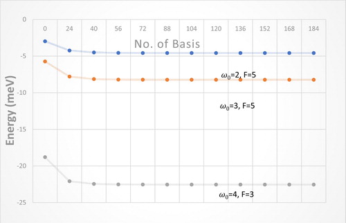
Table 1. The values of the Ground state energy and the number of basis involved in the diagonalization process, for different values of F and ω₀.

No. of basis	Ground state energy (meV)
	F = 5R*	F = 5R*	F = 3R*
No. of basis	ω0 = 2R*	ω0 = 3R*	ω0 = 4R*
0	−2.97591	−2.75044	−13.0569
24	−4.23069	−3.56145	−14.2875
40	−4.4962	−3.63935	−14.3127
56	−4.55723	−3.64566	−14.3131
72	−4.57217	−3.64607	−14.3131
88	−4.57634	−3.64609	−14.3131
104	−4.57758	−3.64609	−14.3131
120	−4.57795	−3.64609	−14.3131
136	−4.57801	−3.64609	−14.3131
152	−4.57807	−3.64609	−14.3131
168	−4.57808	−3.64609	−14.3131
184	−4.57808	−3.64609	−14.3131

We have used in these calculations a Hamiltonian matrix of dimension: 72 × 72 where we have obtained a numerical stability in the ground state energy values as shown in Figure 1. This choice for the dimension of the Hamiltonian matrix: 72 × 72 guarantees that the calculated statistical average energy of the QD system at high temperature is also convergent, as shown in Table 1 of Ref. [38] and Figure 12 of Ref. [39].

Now, we will present the effects of electric field strength (F), temperature (T), confinement frequency (ω₀), tilt angle (θ), and the presence of donor impurity on the statistical energy, magnetization and susceptibility.

In order to obtain our desired results for the magnetic properties of the QD, we computed the statistical energy as an important quantity, from which we can derive all the magneto-thermodynamic quantities, like M and χ, defined in Equations (25) and (26).

The effect of electric field on the statistical energy is plotted in Figure 2. The figure shows that as the electric field strength gets higher, the statistical energy gets lower, because the electric field tries to separate the electron from the donor impurity, thereby, the binding energy gets lower, and so, the statistical energy decreases.

Figure 2. Statistical energy against ω_c for different values of F (F = 4.8R* for solid line, = 7R* for dashed line), ω₀= 2R*, T = 0.01 K, θ = 60°.

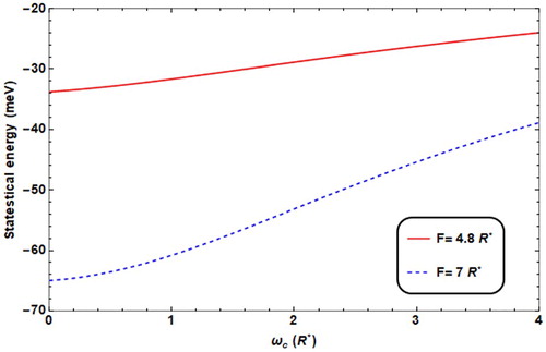
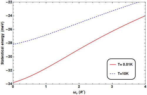
Figure 3 shows the variation of the statistical energy as function of the magnetic field for two different temperatures. The plotted average energy curves show the following behaviour: as the magnetic field strength increases, the statistical energy increases too, and that is due to the additional confinement of the electron by the magnetic field, and for different values of temperature. We can also see from the figure that for higher temperature, the statistical energy is higher, and that is consistent with Reference [40]

Figure 3. Statistical energy against ω_c for different values of T (T = 0.01 K for solid line, =10 K for dashed line), ω₀= 2R*, F = 4.8R*, θ = 60°.

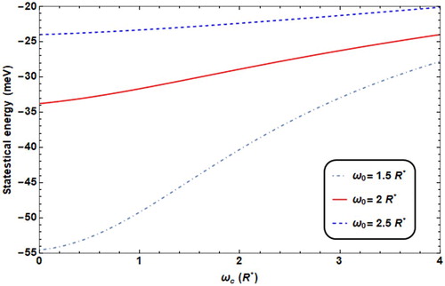
The effect of the parabolic confinement strength ω₀ on the average energy is presented in Figure 4, where we can figure out that ω_c has more profound effect on the statistical energy when ω₀ is lower, on the other hand, when ω₀ is higher, the effect of ω_c is minor. In general, as ω₀ increases, the effective frequency ω_eff enhances the statistical energy.

Figure 4. Statistical energy against ω_c for different values of ω₀ (ω₀ = 2R* for solid line, = 2.5R* for dashed line, = 1.5R* for dot dashed), T = 0.01 K, F = 4.8R*, θ = 60°.

In Figure 5, we have displayed the influence of changing the tilt angle θ on the energy values. As the angle θ increases, the strength of the electric field term also increases, which leads to quite large separation of the electron from the donor impurity. In this case, the binding energy of the donor impurity decreases since the Coulomb attractive energy reduces, (V_c ∼ e²/r) also. In this case, the presence of donor impurity enhances the average statistical energy values. The influence of the donor impurity on the average energy is shown in Figure 6.

Figure 5. Statistical energy against ω_c for different values of θ (θ = 60° for solid line, =36° for thick line, = 0 for dot dashed line), ω₀= 2R*, F = 4.8R*, T = 0.01 K.

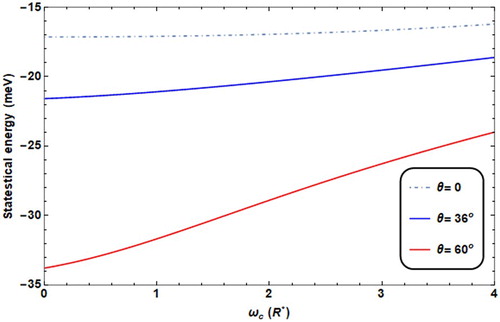
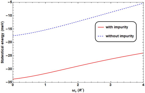
Figure 6. Statistical energy against ω_c with (dashed line)/without (solid line) impurity, ω₀= 2R*, F = 4.8 K, θ = 60°, T = 0.01 K.

To investigate the magnetic quantities of the QD, we present the computed results for the magnetic quantities, M and χ, making use of the corresponding statistical energy $⟨E⟩$ figures shown previously.

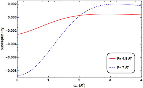
The variation of M as a function of ω_c at various values of F is shown in Figure 7. For both values of electric field strengths F, we have noticed that, as ω_c increases, M decreases (or |M| increases) till ω_c reaches critical value, then it starts to increase. This change means that transition occurs in the magnetic type of the QD material: from -ve χ-value (diamagnetic material) to +ve χ-value (paramagnetic material) as shown in the susceptibility related curves, plotted in Figure 8. For fixed values of ω_c, the magnetization decreases as the electric field strength increases. This result is consistent with the donor energy behaviour against the electric field shown and discussed previously.

Figure 7. Magnetization versus ω_c with different F values (F = 4.8R* for solid line, = 7R* for dashed line), with ω₀= 2R*, T = 0.01 K, θ = 60°.

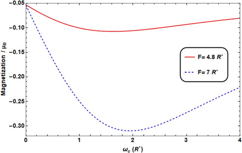
Figure 8. Susceptibility versus ω_c with different F values (F = 4.8R* for solid line, = 7R* for dashed line), with w₀= 2R*, T = 0.01 K, θ = 60°.

The change in the behaviour of M is due to the electric field effect, which leads to the flipping in the sign of χ from diamagnetic (-χ) to paramagnetic material (+χ).

As a result, the electric field strength allows us to tune and control the magnetic type of the QD material.

It is quite the same behaviour of M and consequently of χ that appears when M and χ are plotted against ω_c, as shown in Figures 9 and 10. We observe that for low temperature, the transition from decreasing M case (i.e. diamagnetic region) to the increasing M case (paramagnetic region) occurs at low value of ω_c, while the effect of T appears at high temperature range, where the transition occurs at high magnetic field strength ω_c.

Figure 9. Magnetization versus ω_c with different T values (T = 0.01 K for solid line, = 10K* for dashed line) with ω₀= 2R*, F = 4.8R*, θ = 60°.

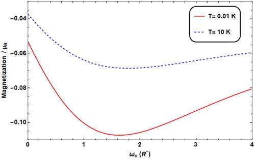
Figure 10. Susceptibility versus ω_c with different T values (T = 0.01 K for solid line, = 10K* for dashed line) with ω₀= 2R*, F = 4.8R*, θ = 60°.

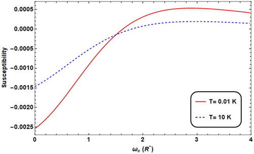
At low magnetic field, the thermal energy is becoming more significant, and it enhances χ as the temperature increases. However, as the magnetic field increases, χ decreases with increasing temperature as expected.

The effects of the parabolic confinement ω₀ on M and χ are presented in Figures 11 and 12, respectively. The transition occurs more quickly for low confinement, while at higher confinement the transition gets slower.

Figure 11. Magnetization versus ω_c with different ω₀ values (ω₀= 2R* for solid line, = 2.5R* for dashed line, = 1.5R* for dot dashed) with T = 0.01 K, F = 4.8R*, θ = 60°.

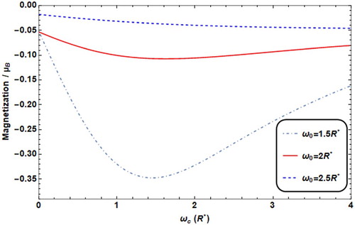
Figure 12. Susceptibility versus ω_c with different ω₀ values (ω₀= 2R* for solid line, = 2.5R* for dashed line, = 1.5R* for dot dashed) with T = 0.01 K, F = 4.8R*, θ = 60°.

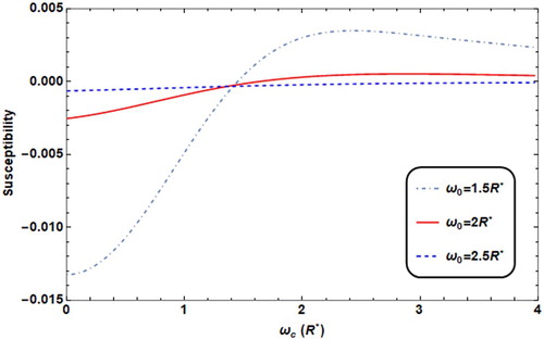
For quite high magnetic field, (ω_c >> 1.5R*), χ is higher for a corresponding high values of ω₀, due to the large confinement of the electron in the QD.

In Figures 13 and 14, the effect of the tilt angle θ on the M and χ is presented. Where increasing θ, this enhances the resultant electric field strength F. So, the behaviour is similar to that in Figures 7 and 8. Noticing that in the absence of electric field (θ = 0), the change in M is smooth and with no peak and χ remains approximately constant in the diamagnetic regime.

Figure 13. Magnetization versus ω_c with different θ values (θ = 60° for solid line, = 36° for thick line, = 0° for dot dashed) with T = 0.01 K, F = 4.8R*, ω₀ = 2R*.

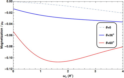
Figure 14. Susceptibility versus ω_c with different θ values (θ = 60° for solid line, = 36° for thick line, = 0° for dot dashed) with T = 0.01 K, F = 4.8R*, ω₀ = 2R*.

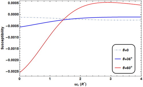
For quite high magnetic field range: (ω_c: 1.5R*-4R*), the susceptibility χ increases as the tilt angle (θ) increases. The increment in (θ) enhances the strength of the electric field, and thus, decreases the donor energy. In this case M decreases while χ increases.

Again, the tilt angle θ is an efficient controlling parameter to the sign of χ.

In addition, we plotted M and χ against ω_c in the presence and absence of donor impurity, and the results are as presented in Figures 15 and 16, respectively. In the presence of donor impurity, the magnetization, M, changes from decreasing into increasing (phase transition from diamagnetic type to paramagnetic one at about ω_c= 1.6R*), however, in the absence of impurity, M decreases until it reaches a saturation limit at about ω_c = 2.5R*, where χ becomes constant. The attractive Coulomb energy due to the electron impurity term lowers the average energy of the confined electron in the QD, which results in reducing the magnetization of the QD, as plotted in Figure 15.

Figure 15. Magnetization versus ω_c with the presence/absence of impurity (solid/dashed) with T = 0.01 K, F = 4.8R*, ω₀ = 2R*, θ = 60°.

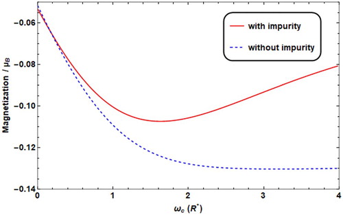
Figure 16. Susceptibility versus ω_c with the presence/absence of impurity (solid/dashed) with T = 0.01 K, F = 4.8R*, ω₀= 2R*, θ = 60°.

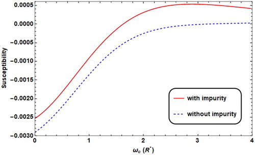
The effect of the impurity on M is very important. The calculations show that the donor impurity decreases the magnetization as we explained in Figure 15, and in this case, the magnetic susceptibility enhances as the magnetic field increases (Figure 16).

4. Conclusion

In conclusion, the Hamiltonian of donor impurity in QD, based on the effective mass approximation, has been solved in the presence of magnetic field and tilted electric field, in addition parabolic confinement potential, using the numerical diagonalization method. We have studied the dependence of the energy levels of the QD as a function of: tilt angle (θ), electric field strength (F) and confinement frequency (ω₀). Our results are in good agreement with reported works. Moreover, the statistical average energy (E) spectra, the magnetization (M) and susceptibility (χ) were computed as a function of our controllable parameters (T, $\theta$, F, ω_c). It was found that increasing F lowers the values of the statistical energy values, which in turn affects M, making it decreases at lower ω_c and increases at higher ω_c more rapidly, which leads to a transition from diamagnetic type to paramagnetic one at lower value of ω_c. The calculation shows that this magnetic phase transition for GaAs material occurs at magnetic field strength $B\approx 5-6.6T$, electric field strength $F\approx 1\text{kV/cm}$, confinement frequency ${\omega }_0\approx 11.5\text{meV}$ angle $\theta$= 60 degrees and temperature T = 0.01 K. Decreasing temperature diminishes E, and the transition from diamagnetic to paramagnetic is more obvious and faster for lower temperature. But for high values of ω₀, the effect of those parameters is minor, where the influence of ω₀ will be dominant.

Disclosure statement

No potential conflict of interest was reported by the authors.

ORCID

Amal Abu Alia http://orcid.org/0000-0003-0734-1433

Mohammad K. Elsaid http://orcid.org/0000-0002-1392-3192

Ayham Shaer http://orcid.org/0000-0002-6518-6470

References

- Harrison P. Quantum wells, wires and dots. Chichester: John Wiley & Sons; 2005.
- Tiwari S, Rana F, Chan K, et al. Single charge and confinement effects in nano-crystal memories. Appl Phys Lett. 1996;69(9):1232–1234. doi: 10.1063/1.117421
- Schwarz JA, Contescu CI, Putyera K. Dekker encyclopedia of nanoscience and nanotechnology. Vol. 3. Boca Raton (FL): CRC Press; 2004.
- Bahramiyan H, Khordad R. Effect of various factors on binding energy of pyramid quantum dot: pressure, temperature and impurity position. Opt Quantum Electron. 2014;46(5):719–729. doi: 10.1007/s11082-013-9782-1
- Xu YB, Hassan SSA, Wong PKJ, et al. Hybrid spintronic structures with magnetic oxides and Heusler alloys. IEEE Trans Magn. 2008;44(11):2959–2965. doi: 10.1109/TMAG.2008.2002188
- Li S-S, Xia J-B. Binding energy of a hydrogenic donor impurity in a rectangular parallelepiped-shaped quantum dot: quantum confinement and stark effects. J Appl Phys. 2007;101(9):093716. doi: 10.1063/1.2734097
- Bose C, Sarkar CK. Effect of a parabolic potential on the impurity binding energy in spherical quantum dots. Phys B Condens Matter. 1998;253(3-4):238–241. doi: 10.1016/S0921-4526(98)00407-4
- Kırak M, Yılmaz S, Shahin M, et al. The electric field effects on the binding energies and the nonlinear optical properties of a donor impurity in a spherical quantum. J Appl Phys. 2011;109(9):094309. doi: 10.1063/1.3582137
- Murillo G, Porras-Montenegro N. Effects of an electric field on the binding energy of a donor impurity in a spherical GaAs quantum dot with parabolic confinement. Phys Stat Solid B. 2000;220(1):187–190. doi: 10.1002/1521-3951(200007)220:1<187::AID-PSSB187>3.0.CO;2-D
- Zeng Z, Garoufalis CS, Baskoutas S. Combination effects of tilted electric and magnetic fields on donor binding energy in a GaAs/AlGaAs cylindrical quantum. J Phys D Appl Phys. 2012;45(23):235102. doi: 10.1088/0022-3727/45/23/235102
- Li YX, Liu JJ, Kong XJ. The effect of a spatially dependent effective mass on hydrogenic impurity binding energy in a finite parabolic quantum well with a magnetic field. J Appl Phys. 2000;88(5):2588–2592. doi: 10.1063/1.1286244
- Wang YJ, Leem YA, McCombe BD, et al. Strong three-level resonant magnetopolaron effect due to the intersubband coupling in heavily modulation-doped GaAs/AlxGa1−xAs single quantum wells at high magnetic fields. Phys Rev B. 2001;64(16):161303. doi: 10.1103/PhysRevB.64.161303
- Niculescu E, Gearba A, Cone G, et al. Magnetic field dependence of the binding energy of shallow donors in GaAs quantum-well wires. Superlattices Microstruct. 2001;29(5):319–328. doi: 10.1006/spmi.2000.0895
- Ham H, Spector HN. Photoionization cross section of hydrogenic impurities in cylindrical quantum wires: finite well model. J Appl Phys. 2006;100(2):024304. doi: 10.1063/1.2211311
- Ham H, Lee CJ, Spector HN. Photoionization cross section of hydrogenic impurities in cylindrical quantum wires: infinite well model. J Appl Phys. 2004;96(1):335–339. doi: 10.1063/1.1759394
- Aktas S, Boz FK, Dalgic SS. Electric and magnetic field effects on the binding energy of a hydrogenic donor impurity in a coaxial quantum well wire. Phys E Low-Dimensional Syst Nanostruct. 2005;28(1):96–105. doi: 10.1016/j.physe.2005.02.002
- An XT, Liu JJ. Hydrogenic impurities in parabolic quantum-well wires in a magnetic field. J Appl Phys. 2006;99(12):123713. doi: 10.1063/1.2206415
- Barati M, Rezaei G, Vahdani MRK. Binding energy of a hydrogenic donor impurity in an ellipsoidal finite-potential quantum dot. Phys Stat Solid B. 2007;244(7):2605–2610. doi: 10.1002/pssb.200642543
- Li SS, Xia JB. Electronic structure and binding energy of a hydrogenic impurity in a hierarchically self-assembled GaAsAlxGa1−x As quantum. J Appl Phys. 2006;100(8):083714. doi: 10.1063/1.2358406
- Jiang L, Wang H, Wu H, et al. External electric field effect on the hydrogenic donor impurity in zinc-blende GaN/AlGaN cylindrical quantum. J Appl Phys. 2009;105(5):053710. doi: 10.1063/1.3080175
- Xia C, Zeng Z, Wei S. Electron and impurity states in GaN/AlGaN coupled quantum dots: effects of electric field and hydrostatic pressure. J Appl Phys. 2010;108(5):054307. doi: 10.1063/1.3481437
- John Peter A. The effect of hydrostatic pressure on binding energy of impurity states in spherical quantum dots. Phys E Low-Dimensional Syst Nanostruct. 2005;28(3):225–229. doi: 10.1016/j.physe.2005.03.018
- Qu F, Santos Jr DR, Azevedo RB, et al. Tunable magnetic property of lateral quantum dot molecules. J Phys Conf Ser. 2011;334:012064. doi: 10.1088/1742-6596/334/1/012064
- Ciftja O. Generalized description of few-electron quantum dots at zero and non-zero magnetic fields. Journal of Physics: Condensed Matter. 2007;19(4):046220.
- Tanaka K. Semiclassical study of the magnetization of a quantum. Ann Phys (N Y). 1998;268(1):31–60. doi: 10.1006/aphy.1998.5824
- Soylu A. The influence of external fields on the energy of two interacting electrons in a quantum. Ann Phys (N Y). 2012;327(12):3048–3062. doi: 10.1016/j.aop.2012.06.008
- Karimi MJ, Rezaei G. Effects of external electric and magnetic fields on the linear and nonlinear intersubband optical properties of finite semi-parabolic quantum dots. Phys B Condens Matter. 2011;406(23):4423–4428. doi: 10.1016/j.physb.2011.08.105
- Wang D, Jin G, Zhang Y, et al. Effect of a tilted electric field on the magnetoexciton ground state in a semiconductor quantum. J Appl Phys. 2009;105(6):063716. doi: 10.1063/1.3088886
- Shaer A, Elsaid M, Elhasan M. The magnetic properties of a quantum dot in a magnetic field. Turkish J Phys. 2016;40(3):209–218. doi: 10.3906/fiz-1510-4
- Hwang T-M, Lin W-W, Wang W-C, et al. Numerical simulation of three-dimensional pyramid quantum. J Comput Phys. 2004;196(1):208–232. doi: 10.1016/j.jcp.2003.10.026
- Johnson HT, Freund LB, Akyuz CD, et al. Finite element analysis of strain effects on electronic and transport properties in quantum dots and wires. J Appl Phys. 1998;84(7):3714–3725. doi: 10.1063/1.368549
- Boda A, Chatterjee A. Transition energies and magnetic properties of a neutral donor complex in a Gaussian GaAs quantum. Superlattices Microstruct. 2016;97:268–276. doi: 10.1016/j.spmi.2016.06.009
- Tojo T, Inui M, Ooi R, et al. Effect of isotropy and anisotropy of the confinement potential on the Rashba spin–orbit interaction for an electron in a two-dimensional quantum dot system. Jpn J Appl Phys. 2017;56(7):075201. doi: 10.7567/JJAP.56.075201
- Sanjeev Kumar D, Mukhopadhyay S, Chatterjee A. Magnetization and susceptibility of a parabolic InAs quantum dot with electron–electron and spin–orbit interactions in the presence of a magnetic field at finite temperature. J Magn Magn Mater. 2016;418:169–174. doi: 10.1016/j.jmmm.2016.02.071
- Weng-Fang X. A two-electron quantum ring under magnetic fields. Commun Theor Phys. 2008;49:1619–1621. doi: 10.1088/0253-6102/49/6/58
- Hao J, Liu J-l. A numerical method for exact diagonalization of semiconductor quantum dot model. Comput Phys Commun. 2010;181:937–949. doi: 10.1016/j.cpc.2010.01.006
- Sharma HK, Boda A, Boyacioglu B, et al. Electronic and magnetic properties of two-electron Gaussian GaAs quantum dot with spin-Zemann term. J Magn Magn Mater. 2019;469:171–177. doi: 10.1016/j.jmmm.2018.07.070
- Baghdasaryan DA, Hayrapetyan DB, Kazaryan EM, et al. Thermal and magnetic properties of electron gas in toroidal quantum. Phys E. 2018;101:1–4. doi: 10.1016/j.physe.2018.03.009
- Nammas FS. Thermodynamic properties of two electron quantum dot with harmonic interaction. Physica. 2018;A508:187–198. doi: 10.1016/j.physa.2018.05.116
- Ghaltaghchyan HT, Kazaryan EM, Sarkisyan A. Diamagnetism in the cylindrical quantum dot with parabolic confinement potential. J Phys Sci. 2016;3:20–24.