Global dynamical properties of two discrete-time exponential systems

Abstract

We explore the global dynamics of following three directional discrete-time exponential systems of difference equations: $x_{n+1}=\frac{{\alpha }_{19}+{\beta }_{19}{e}^{-y_n}}{{\gamma }_{19}+z_{n-1}},y_{n+1}=\frac{{\alpha }_{20}+{\beta }_{20}{e}^{-z_n}}{{\gamma }_{20}+x_{n-1}},z_{n+1}=\frac{{\alpha }_{21}+{\beta }_{21}{e}^{-x_n}}{{\gamma }_{21}+y_{n-1}},$ $x_{n+1}=\frac{{\alpha }_{22}+{\beta }_{22}{e}^{-z_n}}{{\gamma }_{22}+x_{n-1}},y_{n+1}=\frac{{\alpha }_{23}+{\beta }_{23}{e}^{-x_n}}{{\gamma }_{23}+y_{n-1}},z_{n+1}=\frac{{\alpha }_{24}+{\beta }_{24}{e}^{-y_n}}{{\gamma }_{24}+z_{n-1}},$where ${\alpha }_i,{\beta }_i,{\gamma }_i$, $i=19,20,\cdots ,24$ and $x_i,y_i,z_i,i=0,-1$ are belonging to ${\text{R}}^{\ge 0}$. Precisely, we explore the boundedness and persistence of positive solution, existence of invariant rectangle, existence and uniqueness of positive equilibrium point, local and global dynamics about the unique positive equilibrium, and rate of convergence of these discrete-time exponential systems. Finally, theoretical results are verified numerically.

KEYWORDS:

• Difference equations
• stability
• numerical simulations

Mathematics Subject Classifications:

• 39A10
• 40A05

1. Introduction

Global dynamical properties of discrete-time exponential difference equations or systems of difference equations have widely investigated in the recent years. For instance, Ozturk et al. [1] have explored the dynamical properties of following exponential difference equation: (1) $x_{n+1}=\frac{{\alpha }_1+{\alpha }_2{e}^{-x_n}}{{\alpha }_3+x_{n-1}},n=0,1,\cdots ,$(1)

where ${\alpha }_i,i=1,2,3$ and $x_i,i=0,-1$ are belonging to ${\mathbb{R}}^{\ge 0}$. Papaschinopoulos et al. [2] have explored the dynamical properties of following discrete-time exponential systems: (2) $\left.\begin{array}{c}{x}_{n+1}=\frac{{\alpha }_1+{\alpha }_2{e}^{-y_n}}{{\alpha }_3+y_{n-1}},y_{n+1}=\frac{{\alpha }_4+{\alpha }_5{e}^{-x_n}}{{\alpha }_6+x_{n-1}}\\ x_{n+1}=\frac{{\alpha }_1+{\alpha }_2{e}^{-y_n}}{{\alpha }_3+x_{n-1}},y_{n+1}=\frac{{\alpha }_4+{\alpha }_5{e}^{-x_n}}{{\alpha }_6+y_{n-1}}\\ x_{n+1}=\frac{{\alpha }_1+{\alpha }_2{e}^{-x_n}}{{\alpha }_3+y_{n-1}},y_{n+1}=\frac{{\alpha }_4+{\alpha }_5{e}^{-y_n}}{{\alpha }_6+x_{n-1}}\end{array}\right\},$(2)

where ${\alpha }_i,i=1,2,\cdots ,6$ and $x_i,y_i,i=0,-1$ are belonging to ${\mathbb{R}}^{\ge 0}$. Motivated from above studies, we explore the global dynamics of following two three-species discrete-time models which are extension of the work of [1,2]: (3) $\begin{array}{rl}{x}_{n+1}& =\frac{{\alpha }_{19}+{\beta }_{19}{e}^{-y_n}}{{\gamma }_{19}+z_{n-1}},y_{n+1}=\frac{{\alpha }_{20}+{\beta }_{20}{e}^{-z_n}}{{\gamma }_{20}+x_{n-1}},\\ z_{n+1}& =\frac{{\alpha }_{21}+{\beta }_{21}{e}^{-x_n}}{{\gamma }_{21}+y_{n-1}},\end{array}$(3) (4) $\begin{array}{rl}{x}_{n+1}& =\frac{{\alpha }_{22}+{\beta }_{22}{e}^{-z_n}}{{\gamma }_{22}+x_{n-1}},y_{n+1}=\frac{{\alpha }_{23}+{\beta }_{23}{e}^{-x_n}}{{\gamma }_{23}+y_{n-1}},\\ z_{n+1}& =\frac{{\alpha }_{24}+{\beta }_{24}{e}^{-y_n}}{{\gamma }_{24}+z_{n-1}},\end{array}$(4) where ${\alpha }_i,{\beta }_i,{\gamma }_i$, $i=19,20,\cdots ,24$ and $x_i,y_i,z_i,i=0,-1$ are belonging to ${\text{R}}^{\ge 0}$. Discrete-time systems (3) and (4) viewed as models in mathematical biology where biological interpretation of parameters ${\alpha }_i,{\beta }_i,{\gamma }_i$, $i=19,20,\cdots ,24$ are depicted in Table 1:

Table 1. Parameters of the discrete-time models (3) and (4) along their Biological interpretations.

Parameters	Biological interpretations
${\alpha }_{19},{\alpha }_{22}$	Immigration rate of species $x_n$
${\alpha }_{20},{\alpha }_{23}$	Immigration rate of $y_n$
${\alpha }_{21},{\alpha }_{24}$	Immigration rate of $z_n$
${\beta }_{19},{\beta }_{22}$	Growth rate of $x_n$
${\beta }_{20},{\beta }_{23}$	Growth rate of $y_n$
${\beta }_{21},{\beta }_{24}$	Growth rate of $z_n$
${\gamma }_{19},{\gamma }_{22}$	Carrying capacity of $x_n$
${\gamma }_{20},{\gamma }_{23}$	Carrying capacity of $y_n$
${\gamma }_{21},{\gamma }_{24}$	Carrying capacity of $z_n$

Our main contribution in this paper is to explore the global dynamical properties for discrete-time systems (3) and (4). Global dynamics and rate of convergence of (3) are explored in Section 2. This includes the study of boundedness and persistence, existence of invariant rectangle, existence of the unique $+\text{ve}$ equilibrium, global dynamics, and Rate of convergence. Same analysis for system (4) is explored in Section 3. Theoretical results are verified numerically in Section 4. Conclusion is given in Section 5.

2. Dynamics of the system (3)

2.1. Boundedness and persistence

In the following theorem, we explore that every $+ve$ solution $\{\left(x_n,y_n,z_n\right){\}}_{n=-1}^{\mathrm{\infty }}$ of (3) is bounded and persists (see [3,4]).

Theorem 2.1:

The $+ve$ solution $\{\left(x_n,y_n,z_n\right){\}}_{n=-1}^{\mathrm{\infty }}$ of (3) is bounded and persists.

Proof:

If the $+ve$ solution of (3) is $\{\left(x_n,y_n,z_n\right){\}}_{n=-1}^{\mathrm{\infty }}$ then (5) $\begin{array}{rl}{x}_n\le \frac{{\alpha }_{19+}{\beta }_{19}}{{\gamma }_{19}}& =U_{19},y_n\le \frac{{\alpha }_{20+}{\beta }_{20}}{{\gamma }_{20}}\\ & =U_{20},z_n\le \frac{{\alpha }_{21+}{\beta }_{21}}{{\gamma }_{21}}\\ & =U_{21},n=0,1,\cdots .\end{array}$(5) From (3) and (5), one gets (6) $\left.\begin{array}{c}{x}_n\ge \frac{{\alpha }_{19}+{\beta }_{19}{e}^{-\frac{{\alpha }_{20}+{\beta }_{20}}{{\gamma }_{20}}}}{{\gamma }_{19}+{\displaystyle \frac{{\alpha }_{21}+{\beta }_{21}}{{\gamma }_{21}}}}=L_{19}\\ y_n\ge \frac{{\alpha }_{20+}{\beta }_{20}{e}^{-{\displaystyle \frac{{\alpha }_{21}+{\beta }_{21}}{{\gamma }_{21}}}}}{{\gamma }_{20}+{\displaystyle \frac{{\alpha }_{19}+{\beta }_{19}}{{\gamma }_{19}}}}=L_{20}\\ z_n\ge \frac{{\alpha }_{21}+{\beta }_{21}{e}^{-{\displaystyle \frac{{\alpha }_{19}+{\beta }_{19}}{{\gamma }_{19}}}}}{{\gamma }_{21}+{\displaystyle \frac{{\alpha }_{20}+{\beta }_{20}}{{\gamma }_{20}}}}=L_{21}\end{array}\right\},$(6) $n=2,3,\cdots$. Finally from (5) and (6), one gets

$L_{19}\le x_n\le U_{19},L_{20}\le y_n\le U_{20},L_{21}\le z_n\le U_{21},\text{n}=3,4,\cdots$.

2.2. Existence of invariant rectangle

Theorem 2.2:

If $\{\left(x_n,y_n,z_n\right){\}}_{n=-1}^{\mathrm{\infty }}$ is a $+ve$ solution of (3) then its corresponding invariant rectangle is $\left[L_{19},U_{19}\right]\times [L_{20},U_{20}\left]\times \right[L_{21},U_{21}]$ where $\begin{array}{rl}{L}_{19}& =\frac{{\alpha }_{19}+{\beta }_{19}{e}^{-\frac{{\alpha }_{20}+{\beta }_{20}}{{\gamma }_{20}}}}{{\gamma }_{19}+\frac{{\alpha }_{21}+{\beta }_{21}}{{\gamma }_{21}}},U_{19}=\frac{{\alpha }_{19}+{\beta }_{19}}{{\gamma }_{19}},\\ L_{20}& =\frac{{\alpha }_{20}+{\beta }_{20}{e}^{-\frac{{\alpha }_{21}+{\beta }_{21}}{{\gamma }_{21}}}}{{\gamma }_{20}+\frac{{\alpha }_{19}+{\beta }_{19}}{{\gamma }_{19}}},U_{20}=\frac{{\alpha }_{20}+{\beta }_{20}}{{\gamma }_{20}},\\ L_{21}& =\frac{{\alpha }_{21}+{\beta }_{21}{e}^{-\frac{{\alpha }_{19}+{\beta }_{19}}{{\gamma }_{19}}}}{{\gamma }_{21}+\frac{{\alpha }_{20}+{\beta }_{20}}{{\gamma }_{20}}}\mathrm{a}\mathrm{n}\mathrm{d}{U}_{21}=\frac{{\alpha }_{21+}{\beta }_{21}}{{\gamma }_{21}}.\end{array}$

Proof:

Follows by induction.

2.3. Existence of unique $+\text{ve}$ equilibrium, global and local dynamics

Hereafter we will study existence of the $+\text{ve}$ equilibrium, global and local dynamics of (3). It is worthwhile to mentioned that in more general setting, system (3) can also be written as (7) $\begin{array}{rl}{x}_{n+1}& =f\left(y_n,z_{n-1}\right)y_{n+1}=g\left(z_n,x_{n-1}\right),\\ z_{n+1}& =h\left(x_n,y_{n-1}\right).\end{array}$(7)

Lemma 2.1:

Let $\left[a_1,b_1\right],\left[a_2,b_2\right],$ and $\left[a_3,b_3\right]$ be intervals of real numbers, s.t., (8) $\left.\begin{array}{c}f:\left[a_1,b_1\right]\times \left[a_2,b_2\right]\times \left[a_3,b_3\right]\to \left[a_1,b_1\right]\\ g:\left[a_1,b_1\right]\times \left[a_2,b_2\right]\times \left[a_3,b_3\right]\to \left[a_2,b_2\right]\\ h:\left[a_1,b_1\right]\times \left[a_2,b_2\right]\times \left[a_3,b_3\right]\to \left[a_3,b_3\right]\end{array}\right\},$(8) where $f,g$ and $h$ are continuous functions that satisfy the following conditions:

1. Let $f\left(y,z\right)$ is non-increasing $w.r.t.$ $y$(resp.$z$) $\mathrm{\forall }z$(resp.$y$); $g\left(z,x\right)$ is non-increasing $w.r.t$. $z$(resp.$x$) $\mathrm{\forall }x$(resp.$z$) and $h\left(x,y\right)$ is non-increasing $w.r.t.$ $x$(resp.$y$) $\mathrm{\forall }y$(resp.$x$).

2. If$\left(m_1,M_1,m_2,M_2,m_3,M_3\right)\in [a_1,b_1{]}^2\times [a_2,b_2{]}^2\times [a_3,b_3{]}^2$ is a solution of (9) $\left.\begin{array}{cc}{m}_1=f\left(M_2,M_3\right)& M_1=f\left(m_2,m_3\right)\\ m_2=g\left(M_1,M_3\right)& M_2=g\left(m_1,m_3\right)\\ m_3=h\left(M_1,M_2\right)& M_3=h\left(m_1,m_2\right)\end{array}\right\},$(9)

then $m_1=M_1,m_2=M_2,m_3=M_3$. Then (7) has a unique $+ve$ equilibrium $\left(\overline{x},\overline{y},\overline{z}\right)\in \left[a_1,b_1\right]\times \left[a_2,b_2\right]\times \left[a_3,b_3\right]$ and every $+ve$ solution of (7) satisfies (10) $\left.\begin{array}{c}{x}_{n_0}\in \left[a_1,b_1\right],x_{n_0+1}\in \left[a_1,b_1\right]\\ y_{n_0}\in \left[a_2,b_2\right],y_{n_0+1}\in \left[a_2,b_2\right]\\ z_{n_0}\in \left[a_3,b_3\right],z_{n_0+1}\in \left[a_3,b_3\right]\end{array}\right\},$(10) $n_0\in \mathbb{N}$ tends to unique $+ve$ equilibrium $\left(\overline{x},\overline{y},\overline{z}\right)\in \left[a_1,b_1\right]\times \left[a_2,b_2\right]\times \left[a_3,b_3\right]$.

Proof:

Set (11) $\left.\begin{array}{c}{m}_1^{\left(0\right)}=a_1,m_2^{\left(0\right)}=a_2,m_3^{\left(0\right)}=a_3\\ M_1^{\left(0\right)}=b_1,M_2^{\left(0\right)}=b_2,M_3^{\left(0\right)}=b_3\end{array}\right\}.$(11) And for $i=1,2,3,\cdots$, define (12) $\left.\begin{array}{c}{m}_1^{\left(i\right)}=f\left(M_2^{\left(i-1\right)},M_3^{\left(i-1\right)}\right),M_1^{\left(i\right)}\\ =f\left(m_2^{\left(i-1\right)},m_3^{\left(i-1\right)}\right)\\ m_2^{\left(i\right)}=g\left(M_1^{\left(i-1\right)},M_3^{\left(i-1\right)}\right),M_2^{\left(i\right)}\\ =g\left(m_1^{\left(i-1\right)},m_3^{\left(i-1\right)}\right)\\ m_3^{\left(i\right)}=h\left(M_1^{\left(i-1\right)},M_2^{\left(i-1\right)}\right),M_3^{\left(i\right)}\\ =h\left(m_1^{\left(i-1\right)},m_2^{\left(i-1\right)}\right)\end{array}\right\}.$(12) Clearly (13) $\left.\begin{array}{c}{m}_1^{\left(0\right)}\le m_1^{\left(1\right)},m_2^{\left(0\right)}\le m_2^{\left(1\right)},m_3^{\left(0\right)}\le m_3^{\left(1\right)}\\ M_1^{\left(0\right)}\ge M_1^{\left(1\right)},M_2^{\left(0\right)}\ge M_2^{\left(1\right)},M_3^{\left(0\right)}\ge M_3^{\left(1\right)}\end{array}\right\}.$(13) Using the monotonicity of $f,g$ and $h$ one gets (14) $\left.\begin{array}{c}{m}_1^{\left(1\right)}=f\left(M_2^{\left(0\right)},M_3^{\left(0\right)}\right)\le f\left(M_2^{\left(1\right)},M_3^{\left(1\right)}\right)=m_1^{\left(2\right)}\\ m_2^{\left(1\right)}=g\left(M_1^{\left(0\right)},M_3^{\left(0\right)}\right)\le g\left(M_1^{\left(1\right)},M_3^{\left(1\right)}\right)=m_2^{\left(2\right)}\\ m_3^{\left(1\right)}=h\left(M_1^{\left(0\right)},M_2^{\left(0\right)}\right)\le h\left(M_1^{\left(1\right)},M_2^{\left(1\right)}\right)=m_3^{\left(2\right)}\\ M_1^{\left(1\right)}=f\left(m_2^{\left(0\right)},m_3^{\left(0\right)}\right)\ge f\left(m_2^{\left(1\right)},m_3^{\left(1\right)}\right)=M_1^{\left(2\right)}\\ M_2^{\left(1\right)}=g\left(m_1^{\left(0\right)},m_3^{\left(0\right)}\right)\ge g\left(m_1^{\left(1\right)},m_3^{\left(1\right)}\right)=M_2^{\left(2\right)}\\ M_3^{\left(1\right)}=h\left(m_1^{\left(0\right)},m_2^{\left(0\right)}\right)\ge h\left(m_1^{\left(1\right)},m_2^{\left(1\right)}\right)=M_3^{\left(2\right)}\end{array}\right\}.$(14) By induction, we obtain for $i=1,2,3,\cdots$, (15) $\left.\begin{array}{c}{a}_1=m_1^{\left(0\right)}\le m_1^{\left(1\right)}\le \cdots \le m_1^{\left(i\right)}\le \cdots \le \\ M_1^{\left(i\right)}\le \cdots \le M_1^{\left(1\right)}\le M_1^{\left(0\right)}=b_1\\ a_2=m_2^{\left(0\right)}\le m_2^{\left(1\right)}\le \cdots \le m_2^{\left(i\right)}\le \cdots \le \\ M_2^{\left(i\right)}\le \cdots \le M_2^{\left(1\right)}\le M_2^{\left(0\right)}=b_2\\ a_3=m_3^{\left(0\right)}\le m_3^{\left(1\right)}\le \cdots \le m_3^{\left(i\right)}\le \cdots \le \\ M_3^{\left(i\right)}\le \cdots \le M_3^{\left(1\right)}\le M_3^{\left(0\right)}=b_3\end{array}\right\}.$(15) Clearly (16) $\left.\begin{array}{c}{m}_1^{\left(0\right)}\le x_{n_0}\le M_1^{\left(0\right)}\\ m_2^{\left(0\right)}\le y_{n_0}\le M_2^{\left(0\right)}\\ m_3^{\left(0\right)}\le z_{n_0}\le M_3^{\left(0\right)}\end{array}\right\},$(16) which by the monotonicity of $f,g$ and $h$ Implies (17) $\left.\begin{array}{c}{m}_1^{\left(1\right)}=f\left(M_2^{\left(0\right)},M_3^{\left(0\right)}\right)\le x_{n_0+1}=f\left(y_0,z_0\right)\\ \le f\left(m_2^{\left(0\right)},m_3^{\left(0\right)}\right)=M_1^{\left(1\right)}\\ m_2^{\left(1\right)}=g\left(M_1^{\left(0\right)},M_3^{\left(0\right)}\right)\le y_{n_0+1}=g\left(x_0,z_0\right)\\ \le g\left(m_1^{\left(0\right)},m_3^{\left(0\right)}\right)=M_2^{\left(1\right)}\\ m_3^{\left(1\right)}=h\left(M_1^{\left(0\right)},M_2^{\left(0\right)}\right)\le z_{n_0+1}=h\left(x_0,y_0\right)\\ \le h\left(m_1^{\left(0\right)},m_2^{\left(0\right)}\right)=M_3^{\left(1\right)}\\ m_1^{\left(2\right)}=f\left(M_2^{\left(1\right)},M_3^{\left(1\right)}\right)\le x_{n_0+2}=f\left(y_1,z_1\right)\\ \le f\left(m_2^{\left(1\right)},m_3^{\left(1\right)}\right)=M_1^{\left(2\right)}\\ m_2^{\left(2\right)}=g\left(M_1^{\left(1\right)},M_3^{\left(1\right)}\right)\le y_{n_0+2}=g\left(x_1,z_1\right)\\ \le g\left(m_1^{\left(1\right)},m_3^{\left(1\right)}\right)=M_2^{\left(2\right)}\\ m_3^{\left(2\right)}=h\left(M_1^{\left(1\right)},M_2^{\left(1\right)}\right)\le z_{n_0+2}=h\left(x_1,y_1\right)\\ \le h\left(m_1^{\left(1\right)},m_2^{\left(1\right)}\right)=M_3^{\left(2\right)}\end{array}\right\}.$(17) By induction it follows that (18) $\left.\begin{array}{c}{m}_1^{\left(k\right)}\le x_k\le M_1^{\left(k\right)}\\ m_2^{\left(k\right)}\le y_k\le M_2^{\left(k\right)}\\ m_3^{\left(k\right)}\le z_k\le M_3^{\left(k\right)}\end{array}\right\}.$(18) Thus for every $k=0,1,\cdots$, there exist numbers $m_1,m_2,m_3,M_1,M_2,M_3$, $s.t.$, (19) $\left.\begin{array}{c}{m}_1=\underset{k\to \mathrm{\infty }}{lim}{m}_1^{\left(k\right)},m_2=\underset{k\to \mathrm{\infty }}{lim}{m}_2^{\left(k\right)},\\ m_3=\underset{k\to \mathrm{\infty }}{lim}{m}_3^{\left(k\right)}\\ M_1=\underset{k\to \mathrm{\infty }}{lim}{M}_1^{\left(k\right)},M_2=\underset{k\to \mathrm{\infty }}{lim}{M}_2^{\left(k\right)},\\ M_3=\underset{k\to \mathrm{\infty }}{lim}{M}_3^{\left(k\right)}\end{array}\right\}.$(19) Clearly (20) $\left.\begin{array}{c}{m}_1\le \underset{k\to \mathrm{\infty }}{\underset{\_}{\text{lim}}}{x}_k\le \underset{k\to \mathrm{\infty }}{\overline{\text{lim}}}{x}_k\le M_1\\ m_2\le \underset{k\to \mathrm{\infty }}{\underset{\_}{\text{lim}}}{y}_k\le \underset{k\to \mathrm{\infty }}{\overline{\text{lim}}}{y}_k\le M_2\\ m_3\le \underset{k\to \mathrm{\infty }}{\underset{\_}{\text{lim}}}{z}_k\le \underset{k\to \mathrm{\infty }}{\overline{\text{lim}}}{z}_k\le M_3\end{array}\right\}.$(20) Using the continuity of $f,g$ and $h$, equation (12) then implies that (21) $\left.\begin{array}{c}{m}_1=f\left(M_2,M_3\right),M_1=f\left(m_2,m_3\right)\\ m_2=g\left(M_1,M_3\right),M_2=g\left(m_1,m_3\right)\\ m_3=h\left(M_1,M_2\right),M_3=h(m_1,m_2\end{array}\right\}.$(21) By assumption (b) one gets: $m_1=M_1=\overline{x},m_2=M_2=\overline{y},m_3=M_3=\overline{z}$.

Hereafter based on Lemma 2.1, we will prove the following Theorem:

Theorem 2.3:

If (22) ${\beta }_{19}{\beta }_{20}{\beta }_{21}<{\gamma }_{19}{\gamma }_{20}{\gamma }_{21},$(22) then ${\mathrm{\Gamma }}_1=\left(\overline{x},\overline{y},\overline{z}\right)\in \left[L_{19},U_{19}\right]\times [L_{20},U_{20}\left]\times \right[L_{21},U_{21}]$ is the unique $+ve$ equilibrium of (3) and every $+ve$ solution of (3) tends to ${\mathrm{\Gamma }}_1$ of (3) as $n\to \mathrm{\infty }$.

Proof:

From (3) one has (23) $\begin{array}{rl}f\left(y,z\right)& =\frac{{\alpha }_{19}+{\beta }_{19}{e}^{-y}}{{\gamma }_{19}+z},g\left(x,z\right)=\frac{{\alpha }_{20}+{\beta }_{20}{e}^{-z}}{{\gamma }_{20}+x},\\ h\left(x,y\right)& =\frac{{\alpha }_{21}+{\beta }_{21}{e}^{-x}}{{\gamma }_{21}+y}.\end{array}$(23) It is clear that $f,g$ and $h$ satisfies the hypothesis of Lemma 2.1 and let $m_1,m_2,m_3,M_1,M_2,M_3$ be positive numbers, s.t., (24) $\left.\begin{array}{c}{m}_1=\frac{{\alpha }_{19}+{\beta }_{19}{e}^{-M_2}}{{\gamma }_{19}+M_3},M_1=\frac{{\alpha }_{19}+{\beta }_{19}{e}^{-m_2}}{{\gamma }_{19}+m_3}\\ m_2=\frac{{\alpha }_{20}+{\beta }_{20}{e}^{-M_3}}{{\gamma }_{20}+M_1},M_2=\frac{{\alpha }_{20}+{\beta }_{20}{e}^{-m_3}}{{\gamma }_{20}+m_1}\\ m_3=\frac{{\alpha }_{21}+{\beta }_{21}{e}^{-M_1}}{{\gamma }_{21}+M_2},M_3=\frac{{\alpha }_{21}+{\beta }_{21}{e}^{-m_1}}{{\gamma }_{21}+m_2}\end{array}\right\}.$(24) From (24) one gets (25) $\left.\begin{array}{cc}{e}^{-M_2}& =\frac{m_1\left({\gamma }_{19}+M_3\right)-{\alpha }_{19}}{{\beta }_{19}},e^{-m_2}\\ & =\frac{M_1\left({\gamma }_{19}+m_3\right)-{\alpha }_{19}}{{\beta }_{19}}\\ e^{-M_3}& =\frac{m_2\left({\gamma }_{20}+M_1\right)-{\alpha }_{20}}{{\beta }_{20}},e^{-m_3}\\ & =\frac{M_2\left({\gamma }_{20}+m_1\right)-{\alpha }_{20}}{{\beta }_{20}}\\ e^{-M_1}& =\frac{m_3\left({\gamma }_{21}+M_2\right)-{\alpha }_{21}}{{\beta }_{21}},e^{-m_1}\\ & =\frac{M_3\left({\gamma }_{21}+m_2\right)-{\alpha }_{21}}{{\beta }_{21}}\end{array}\right\},$(25) which implies that (26) $\left.\begin{array}{c}{m}_1-M_1=\frac{{\beta }_{19}}{{\gamma }_{19}}\left(e^{-M_2}-e^{-m_2}\right)\\ =\frac{{\beta }_{19}}{{\gamma }_{19}}{e}^{-M_2-m_2}\left(e^{m_2}-e^{M_2}\right)\\ m_2-M_2=\frac{{\beta }_{20}}{{\gamma }_{20}}\left(e^{-M_3}-e^{-m_3}\right)\\ =\frac{{\beta }_{20}}{{\gamma }_{20}}{e}^{-M_3-m_3}\left(e^{m_3}-e^{M_3}\right)\\ m_3-M_3=\frac{{\beta }_{21}}{{\gamma }_{21}}\left(e^{-M_1}-e^{-m_1}\right)\\ =\frac{{\beta }_{21}}{{\gamma }_{21}}{e}^{-M_1-m_1}\left(e^{m_1}-e^{M_1}\right)\end{array}\right\}.$(26) Moreover one gets (27) $\left.\begin{array}{c}{e}^{m_2}-e^{M_2}=e^{\zeta }\left(m_2-M_2\right),\\ \text{min}\left\{m_2,M_2\right\}\le \zeta \le max\left\{m_2,M_2\right\}\\ e^{m_3}-e^{M_3}=e^{\theta }\left(m_3-M_3\right),\\ \text{min}\left\{m_3,M_3\right\}\le \theta \le max\left\{m_3,M_3\right\}\\ e^{m_1}-e^{M_1}=e^{\eta }\left(m_1-M_1\right),\\ \text{min}\left\{m_1,M_1\right\}\le \eta \le max\left\{m_1,M_1\right\}\end{array}\right\}.$(27) In view of (27), equation (26) then implies that (28) $\left.\begin{array}{c}{m}_1-M_1=\frac{{\beta }_{19}}{{\gamma }_{19}}{e}^{-M_2-m_2+\zeta }\left(m_2-M_2\right)\\ m_2-M_2=\frac{{\beta }_{20}}{{\gamma }_{20}}{e}^{-M_3-m_3+\theta }\left(m_3-M_3\right)\\ m_3-M_3=\frac{{\beta }_{21}}{{\gamma }_{21}}{e}^{-M_1-m_1+\eta }\left(m_1-M_1\right)\end{array}\right\}.$(28) From (28) one gets (29) $\left.\begin{array}{c}|m_1-M_1|\le \frac{{\beta }_{19}}{{\gamma }_{19}}|m_2-M_2|\\ |m_2-M_2|\le \frac{{\beta }_{20}}{{\gamma }_{20}}|m_3-M_3|\\ |m_3-M_3|\le \frac{{\beta }_{21}}{{\gamma }_{21}}|m_1-M_1|\end{array}\right\}.$(29) From (22) and (29) one gets (30) $\left.\begin{array}{c}\left(1-\frac{{\beta }_{19}{\beta }_{20}{\beta }_{21}}{{\gamma }_{19}{\gamma }_{20}{\gamma }_{21}}\right)|m_1-M_1|\le 0\\ \left(1-\frac{{\beta }_{19}{\beta }_{20}{\beta }_{21}}{{\gamma }_{19}{\gamma }_{20}{\gamma }_{21}}\right)|m_2-M_2|\le 0\\ \left(1-\frac{{\beta }_{19}{\beta }_{20}{\beta }_{21}}{{\gamma }_{19}{\gamma }_{20}{\gamma }_{21}}\right)|m_3-M_3|\le 0\end{array}\right\}.$(30) Finally equation (30) then implies that $m_1=M_1,m_2=M_2$ and $m_3=M_3$. Therefore from (5) and (6) and statement (b) of Lemma 2.1, (3) has a unique $+ve$ equilibrium ${\mathrm{\Gamma }}_1$ and every $+ve$ solution of (3) tends to ${\mathrm{\Gamma }}_1$ as $n\to \mathrm{\infty }$.

Hereafter global dynamics of (3) about ${\mathrm{\Gamma }}_1$ is investigated.

Theorem 2.4:

Assume that (22) hold and if (31) $\begin{array}{rl}& \frac{1}{{\gamma }_{19}+L_{21}}\left(\frac{{\beta }_{19}{e}^{-L_{20}}\left({\alpha }_{20}+{\beta }_{20}{e}^{-L_{21}}\right)}{{({\gamma }_{20}+L_{19})}^2}\right.\\ & \left.+\frac{{\beta }_{21}{e}^{-L_{19}}\left({\alpha }_{19}+{\beta }_{19}{e}^{-L_{20}}\right)}{\left({\gamma }_{19}+L_{21}\right)\left({\gamma }_{21}+L_{20}\right)}\right)\\ & +\frac{{\beta }_{20}{e}^{-L_{21}}\left({\alpha }_{21}+{\beta }_{21}{e}^{-L_{19}}\right)}{\left({\gamma }_{20}+L_{19}\right){({\gamma }_{21}+L_{20})}^2}\\ & +\frac{1}{\left({\gamma }_{19}+L_{21}\right)\left({\gamma }_{20}+L_{19}\right)\left({\gamma }_{21}+L_{20}\right)}\\ & \left(\begin{array}{c}{\beta }_{19}{\beta }_{20}{\beta }_{21}{e}^{-L_{19}-L_{20}-L_{21}}+\\ \times \frac{\begin{array}{c}\left({\alpha }_{19}+{\beta }_{19}{e}^{-L_{20}}\right)\left({\alpha }_{20}+{\beta }_{20}{e}^{-L_{21}}\right)\\ \left({\alpha }_{21}+{\beta }_{21}{e}^{-L_{19}}\right)\end{array}}{\left({\gamma }_{19}+L_{21}\right)\left({\gamma }_{20}+L_{19}\right)\left({\gamma }_{21}+L_{20}\right)}\end{array}\right)<1,\end{array}$(31) then ${\mathrm{\Gamma }}_1$ of (3) is globally asymptotically stable.

Proof:

Jacobian matrix $J_{{\mathrm{\Gamma }}_1}$ about ${\mathrm{\Gamma }}_1$ is (32) $J_{{\mathrm{\Gamma }}_1}=\left(\begin{array}{cccccc}0& 0& A_1& 0& 0& A_2\\ 1& 0& 0& 0& 0& 0\\ 0& B_1& 0& 0& B_2& 0\\ 0& 0& 1& 0& 0& 0\\ C_1& 0& 0& C_2& 0& 0\\ 0& 0& 0& 0& 1& 0\end{array}\right),$(32) where (33) $\left.\begin{array}{c}{A}_1=\frac{-{\beta }_{19}{e}^{-\overline{y}}}{{\gamma }_{19}+\overline{z}},A_2=-\frac{{\alpha }_{19}+{\beta }_{19}{e}^{-\overline{y}}}{{({\gamma }_{19}+\overline{z})}^2},\\ B_1=-\frac{{\alpha }_{20}+{\beta }_{20}{e}^{-\overline{z}}}{{({\gamma }_{20}+\overline{x})}^2},B_2=-\frac{{\beta }_{20}{e}^{-\overline{z}}}{{\gamma }_{20}+\overline{x}},\\ C_1=-\frac{{\beta }_{21}{e}^{-\overline{x}}}{{\gamma }_{21}+\overline{y}},C_2=-\frac{{\alpha }_{21}+{\beta }_{21}{e}^{-\overline{x}}}{{({\gamma }_{21}+\overline{y})}^2}\end{array}\right\}.$(33) Moreover Characteristic equation of $J_{{\mathrm{\Gamma }}_1}$ about ${\mathrm{\Gamma }}_1$ is given by (34) ${\lambda }^6+{\mu }_1{\lambda }^3+{\mu }_2=0,$(34) where (35) $\begin{array}{rl}{\mu }_1& =-\left(A_1{B}_1+A_2{C}_1+A_1{B}_2{C}_1+B_2{C}_2\right),\\ {\mu }_2& =-A_2{B}_1{C}_2.\end{array}$(35) Now (36) $\begin{array}{rl}& \sum _{i=1}^2|{\mu }_i|\\ & =\frac{{\beta }_{19}{e}^{-\overline{y}}\left({\alpha }_{20}+{\beta }_{20}{e}^{-\overline{z}}\right)}{\left({\gamma }_{19}+\overline{z}\right){({\gamma }_{20}+\overline{x})}^2}\\ & +\frac{{\beta }_{19}{\beta }_{20}{\beta }_{21}{e}^{-\overline{x}-\overline{y}-\overline{z}}}{\left({\gamma }_{19}+\overline{z}\right)\left({\gamma }_{20}+\overline{x}\right)\left({\gamma }_{21}+\overline{y}\right)}\\ & +\frac{{\beta }_{21}{e}^{-\overline{x}}\left({\alpha }_{19}+{\beta }_{19}{e}^{-\overline{y}}\right)}{{({\gamma }_{19}+\overline{z})}^2\left({\gamma }_{21}+\overline{y}\right)}\\ & +\frac{{\beta }_{20}{e}^{-\overline{z}}\left({\alpha }_{21}+{\beta }_{21}{e}^{-\overline{x}}\right)}{\left({\gamma }_{20}+\overline{x}\right){({\gamma }_{21}+\overline{y})}^2}\\ & \times \frac{\begin{array}{c}\left({\alpha }_{19}+{\beta }_{19}{e}^{-\overline{y}}\right)\left({\alpha }_{20}+{\beta }_{20}{e}^{-\overline{z}}\right)\\ \left({\alpha }_{21}+{\beta }_{21}{e}^{-\overline{x}}\right)\end{array}}{{({\gamma }_{19}+\overline{z})}^2{({\gamma }_{20}+\overline{x})}^2{({\gamma }_{21}+\overline{y})}^2},\\ & \le \frac{{\beta }_{19}{\beta }_{20}{\beta }_{21}{e}^{-L_{19}-L_{20}-L_{21}}}{\left({\gamma }_{19}+L_{21}\right)\left({\gamma }_{20}+L_{19}\right)\left({\gamma }_{21}+L_{20}\right)}\\ & +\frac{{\beta }_{19}{e}^{-L_{20}}\left({\alpha }_{20}+{\beta }_{20}{e}^{-L_{21}}\right)}{\left({\gamma }_{19}+L_{21}\right){({\gamma }_{20}+L_{19})}^2}\\ & +\frac{{\beta }_{21}{e}^{-L_{19}}\left({\alpha }_{19}+{\beta }_{19}{e}^{-L_{20}}\right)}{{({\gamma }_{19}+L_{21})}^2\left({\gamma }_{21}+L_{20}\right)}\\ & +\frac{{\beta }_{20}{e}^{-L_{21}}\left({\alpha }_{21}+{\beta }_{21}{e}^{-L_{19}}\right)}{\left({\gamma }_{20}+L_{19}\right){({\gamma }_{21}+L_{20})}^2}\\ & \times \frac{\begin{array}{c}\left({\alpha }_{19}+{\beta }_{19}{e}^{-L_{20}}\right)\left({\alpha }_{20}+{\beta }_{20}{e}^{-L_{21}}\right)\\ \left({\alpha }_{21}+{\beta }_{21}{e}^{-L_{19}}\right)\end{array}}{{({\gamma }_{19}+L_{21})}^2{({\gamma }_{20}+L_{19})}^2{({\gamma }_{21}+L_{20})}^2},\\ & =\frac{1}{{\gamma }_{19}+L_{21}}\left(\frac{{\beta }_{19}{e}^{-L_{20}}\left({\alpha }_{20}+{\beta }_{20}{e}^{-L_{21}}\right)}{{({\gamma }_{20}+L_{19})}^2}\right.\\ & \left.+\frac{{\beta }_{21}{e}^{-L_{19}}\left({\alpha }_{19}+{\beta }_{19}{e}^{-L_{20}}\right)}{\left({\gamma }_{19}+L_{21}\right)\left({\gamma }_{21}+L_{20}\right)}\right)\\ & +\frac{{\beta }_{20}{e}^{-L_{21}}\left({\alpha }_{21}+{\beta }_{21}{e}^{-L_{19}}\right)}{\left({\gamma }_{20}+L_{19}\right){({\gamma }_{21}+L_{20})}^2}\\ & +\frac{1}{\left({\gamma }_{19}+L_{21}\right)\left({\gamma }_{20}+L_{19}\right)\left({\gamma }_{21}+L_{20}\right)}\\ & \times \left(\begin{array}{c}{\beta }_{19}{\beta }_{20}{\beta }_{21}{e}^{-L_{19}-L_{20}-L_{21}}+\left({\alpha }_{19}+{\beta }_{19}{e}^{-L_{20}}\right)\\ \frac{\left({\alpha }_{20}+{\beta }_{20}{e}^{-L_{21}}\right)\left({\alpha }_{21}+{\beta }_{21}{e}^{-L_{19}}\right)}{\left({\gamma }_{19}+L_{21}\right)\left({\gamma }_{20}+L_{19}\right)\left({\gamma }_{21}+L_{20}\right)}\end{array}\right).\end{array}$(36) Assuming condition (31) holds then from (36) one get ${\sum }_{i=1}^2|{\mu }_i|<1$ and hence Theorem 1.5 of [5] implies that ${\mathrm{\Gamma }}_1$ of (3) is locally asymptotically stable. Moreover by Theorem 2.3, ${\mathrm{\Gamma }}_1$ of (3) is globally asymptotically stable.

Hereafter Rate of convergence about ${\mathrm{\Gamma }}_1$ of (3) is investigated motivated from the work of [6].

2.4. Rate of convergence

Theorem 2.5:

If $\{\left(x_n,y_n,z_n\right){\}}_{n=-1}^{\mathrm{\infty }}$ is a $+ve$ solution of (3), s.t.,. (37) $\left.\begin{array}{c}\underset{n\to \mathrm{\infty }}{\mathrm{l}\mathrm{i}\mathrm{m}}{x}_n=\overline{x}\\ \underset{n\to \mathrm{\infty }}{\mathrm{l}\mathrm{i}\mathrm{m}}{y}_n=\overline{y}\\ \underset{n\to \mathrm{\infty }}{\mathrm{l}\mathrm{i}\mathrm{m}}{z}_n=\overline{z}\end{array}\right\},$(37) where (38) $\left.\begin{array}{c}\overline{x}\in \left[L_{19},U_{19}\right]\\ \overline{y}\in \left[L_{20},U_{20}\right]\\ \overline{z}\in \left[L_{21},U_{21}\right]\end{array}\right\}.$(38) Then error vector $e_n=(e_n^{19},e_{n-1}^{19},e_n^{20},e_{n-1}^{20},e_n^{21},e_{n-1}^{21}{)}^T$ of every $+ve$ solution of (3) satisfying (39) $\left.\begin{array}{c}\underset{n\to \mathrm{\infty }}{\text{lim}}(\parallel e_n\parallel {)}^{\frac{1}{n}}=|{\lambda }_{1,2,3,4,5,6}{J}_{{\mathrm{\Gamma }}_1}|\\ \underset{n\to \mathrm{\infty }}{\text{lim}}\frac{\parallel e_{n+1}\parallel }{\parallel e_n\parallel }=|{\lambda }_{1,2,3,4,5,6}{J}_{{\mathrm{\Gamma }}_1}|\end{array}\right\},$(39) where $|{\lambda }_{1,2,3,4,5,6}{J}_{{\mathrm{\Gamma }}_1}|$ are the Characteristic Root of $J_{{\mathrm{\Gamma }}_1}$.

Proof:

If $\{\left(x_n,y_n,z_n\right){\}}_{n=-1}^{\mathrm{\infty }}$ is a $+ve$ solution of (3), s.t., (37) along with (38) hold. For error terms one has (40) $\begin{array}{r}\left.\begin{array}{c}{x}_{n+1}-\overline{x}=\frac{{\alpha }_{19}+{\beta }_{19}{e}^{-y_n}}{{\gamma }_{19}+z_{n-1}}-\frac{{\alpha }_{19}+{\beta }_{19}{e}^{-\overline{y}}}{{\gamma }_{19}+\overline{z}}\\ =\frac{{\beta }_{19}\left(e^{-y_n}-e^{-\overline{y}}\right)}{\left({\gamma }_{19}+z_{n-1}\right)\left(y_n-\overline{y}\right)}\left(y_n-\overline{y}\right)\\ -\frac{{\alpha }_{19}+{\beta }_{19}{e}^{-\overline{y}}}{\left({\gamma }_{19}+z_{n-1}\right)\left({\gamma }_{19}+\overline{z}\right)}\left(z_{n-1}-\overline{z}\right)\\ y_{n+1}-\overline{y}=\frac{{\alpha }_{20}+{\beta }_{20}{e}^{-z_n}}{{\gamma }_{20}+x_{n-1}}-\frac{{\alpha }_{20}+{\beta }_{20}{e}^{-\overline{z}}}{{\gamma }_{20}+\overline{x}}\\ =\frac{{\beta }_{20}\left(e^{-z_n}-e^{-\overline{z}}\right)}{\left({\gamma }_{20}+x_{n-1}\right)\left(z_n-\overline{z}\right)}\left(z_n-\overline{z}\right)\\ -\frac{{\alpha }_{20}+{\beta }_{20}{e}^{-\overline{z}}}{\left({\gamma }_{20}+x_{n-1}\right)\left({\gamma }_{20}+\overline{x}\right)}\left(x_{n-1}-\overline{x}\right)\\ z_{n+1}-\overline{z}=\frac{{\alpha }_{21}+{\beta }_{21}{e}^{-x_n}}{{\gamma }_{21}+y_{n-1}}-\frac{{\alpha }_{21}+{\beta }_{21}{e}^{-\overline{x}}}{{\gamma }_{21}+\overline{y}}\\ =\frac{{\beta }_{21}\left(e^{-x_n}-e^{-\overline{x}}\right)}{\left({\gamma }_{21}+y_{n-1}\right)\left(x_n-\overline{x}\right)}\left(x_n-\overline{x}\right)\\ -\frac{{\alpha }_{21}+{\beta }_{21}{e}^{-\overline{x}}}{\left({\gamma }_{21}+y_{n-1}\right)\left({\gamma }_{21}+\overline{y}\right)}\left(y_{n-1}-\overline{y}\right)\end{array}\right\},\end{array}$(40) that is (41) $\left.\begin{array}{c}{x}_{n+1}-\overline{x}=\frac{{\beta }_{19}\left(e^{-y_n}-e^{-\overline{y}}\right)}{\left({\gamma }_{19}+z_{n-1}\right)\left(y_n-\overline{y}\right)}\left(y_n-\overline{y}\right)\\ -\frac{{\alpha }_{19}+{\beta }_{19}{e}^{-\overline{y}}}{\left({\gamma }_{19}+z_{n-1}\right)\left({\gamma }_{19}+\overline{z}\right)}\left(z_{n-1}-\overline{z}\right)\\ y_{n+1}-\overline{y}=\frac{{\beta }_{20}\left(e^{-z_n}-e^{-\overline{z}}\right)}{\left({\gamma }_{20}+x_{n-1}\right)\left(z_n-\overline{z}\right)}\left(z_n-\overline{z}\right)\\ -\frac{{\alpha }_{20}+{\beta }_{20}{e}^{-\overline{z}}}{\left({\gamma }_{20}+x_{n-1}\right)\left({\gamma }_{20}+\overline{x}\right)}\left(x_{n-1}-\overline{x}\right)\\ z_{n+1}-\overline{z}=\frac{{\beta }_{21}\left(e^{-x_n}-e^{-\overline{x}}\right)}{\left({\gamma }_{21}+y_{n-1}\right)\left(x_n-\overline{x}\right)}\left(x_n-\overline{x}\right)\\ -\frac{{\alpha }_{21}+{\beta }_{21}{e}^{-\overline{x}}}{\left({\gamma }_{21}+y_{n-1}\right)\left({\gamma }_{21}+\overline{y}\right)}\left(y_{n-1}-\overline{y}\right)\end{array}\right\}.$(41) Set (42) $\left.\begin{array}{c}{e}_n^{19}=x_n-\overline{x}\\ e_n^{20}=y_n-\overline{y}\\ e_n^{21}=z_n-\overline{z}\end{array}\right\}.$(42) By (42), (41) gives (43) $\left.\begin{array}{c}{e}_{n+1}^{19}=a_n{e}_n^{20}+b_n{e}_{n-1}^{21}\\ e_{n+1}^{20}=c_n{e}_{n-1}^{19}+d_n{e}_n^{21}\\ e_{n+1}^{21}=e_n{e}_n^{19}+f_n{e}_{n-1}^{20}\end{array}\right\},$(43) where (44) $\left.\begin{array}{c}{a}_n=\frac{{\beta }_{19}\left(e^{-y_n}-e^{-\overline{y}}\right)}{\left({\gamma }_{19}+z_{n-1}\right)\left(y_n-\overline{y}\right)},\\ b_n=-\frac{{\alpha }_{19}+{\beta }_{19}{e}^{-\overline{y}}}{\left({\gamma }_{19}+z_{n-1}\right)\left({\gamma }_{19}+\overline{z}\right)},\\ c_n=-\frac{{\alpha }_{20}+{\beta }_{20}{e}^{-\overline{z}}}{\left({\gamma }_{20}+x_{n-1}\right)\left({\gamma }_{20}+\overline{x}\right)},\\ d_n=\frac{{\beta }_{20}\left(e^{-z_n}-e^{-\overline{z}}\right)}{\left({\gamma }_{20}+x_{n-1}\right)\left(z_n-\overline{z}\right)},\\ e_n=\frac{{\beta }_{21}\left(e^{-x_n}-e^{-\overline{x}}\right)}{\left({\gamma }_{21}+y_{n-1}\right)\left(x_n-\overline{x}\right)},\\ f_n=-\frac{{\alpha }_{21}+{\beta }_{21}{e}^{-\overline{x}}}{\left({\gamma }_{21}+y_{n-1}\right)\left({\gamma }_{21}+\overline{y}\right)}\end{array}\right\}.$(44) Taking the limits of $a_n,b_n,c_n,d_n,e_{n}and{f}_n$ one gets (45) $\left.\begin{array}{c}\underset{n\to \mathrm{\infty }}{\text{lim}}{a}_n=-\frac{{\beta }_{19}{e}^{-\overline{y}}}{{\gamma }_{19}+\overline{z}},\underset{n\to \mathrm{\infty }}{\text{lim}}{b}_n=-\frac{{\alpha }_{19}+{\beta }_{19}{e}^{-\overline{y}}}{{\left({\gamma }_{19}+\overline{z}\right)}^2},\\ \underset{n\to \mathrm{\infty }}{\text{lim}}{c}_n=-\frac{{\alpha }_{20}+{\beta }_{20}{e}^{-\overline{z}}}{{\left({\gamma }_{20}+\overline{x}\right)}^2},\underset{n\to \mathrm{\infty }}{\text{lim}}{d}_n=-\frac{{\beta }_{20}{e}^{-\overline{z}}}{{\gamma }_{20}+\overline{x}},\\ \underset{n\to \mathrm{\infty }}{\text{lim}}{e}_n=-\frac{{\beta }_{21}{e}^{-\overline{x}}}{{\gamma }_{21}+\overline{y}},\underset{n\to \mathrm{\infty }}{\text{lim}}{f}_n=-\frac{{\alpha }_{21}+{\beta }_{21}{e}^{-\overline{x}}}{{\left({\gamma }_{21}+\overline{y}\right)}^2}\end{array}\right\},$(45) that is (46) $\left.\begin{array}{c}{a}_n=-\frac{{\beta }_{19}{e}^{-\overline{y}}}{{\gamma }_{19}+\overline{z}}+\alpha {20}_n,b_n=-\frac{{\alpha }_{19}+{\beta }_{19}{e}^{-\overline{y}}}{{\left({\gamma }_{19}+\overline{z}\right)}^2}\\ +\alpha {21}_{n-1},c_n=-\frac{{\alpha }_{20}+{\beta }_{20}{e}^{-\overline{z}}}{{\left({\gamma }_{20}+\overline{x}\right)}^2}+\alpha {19}_{n-1}\\ d_n=-\frac{{\beta }_{20}{e}^{-\overline{z}}}{{\gamma }_{20}+\overline{x}}+\alpha {21}_n,e_n=-\frac{{\beta }_{21}{e}^{-\overline{x}}}{{\gamma }_{21}+\overline{y}}\\ +\alpha {19}_n,f_n=-\frac{{\alpha }_{21}+{\beta }_{21}{e}^{-\overline{x}}}{{\left({\gamma }_{21}+\overline{y}\right)}^2}+\alpha {20}_{n-1}\end{array}\right\},$(46) where $\alpha {19}_n,\alpha {19}_{n-1},\alpha {20}_n,\alpha {20}_{n-1},\alpha {21}_n,\alpha {21}_{n-1}\to 0$ as $n\to \mathrm{\infty }$. Now we have system (1.10) of [7], where (47) $\begin{array}{r}A=\left(\begin{array}{ccc}0& 0& -\frac{{\beta }_{19}{e}^{-\overline{y}}}{{\gamma }_{19}+\overline{z}}\\ 1& 0& 0\\ 0& -\frac{{\alpha }_{20}+{\beta }_{20}{e}^{-\overline{z}}}{{\left({\gamma }_{20}+\overline{x}\right)}^2}& 0\\ 0& 0& 1\\ -\frac{{\beta }_{21}{e}^{-\overline{x}}}{{\gamma }_{21}+\overline{y}}& 0& 0\\ 0& 0& 0\end{array}\right.\\ \left.\begin{array}{ccc}0& 0& -\frac{{\alpha }_{19}+{\beta }_{19}{e}^{-\overline{y}}}{{\left({\gamma }_{19}+\overline{z}\right)}^2}\\ 0& 0& 0\\ 0& -\frac{{\beta }_{20}{e}^{-\overline{z}}}{{\gamma }_{20}+\overline{x}}& 0\\ 0& 0& 0\\ -\frac{{\alpha }_{21}+{\beta }_{21}{e}^{-\overline{x}}}{{\left({\gamma }_{21}+\overline{y}\right)}^2}& 0& 0\\ 0& 1& 0\end{array}\right),\end{array}$(47) and (48) $B\left(n\right)=\left(\begin{array}{cccccc}0& 0& \alpha {20}_n& 0& 0& \alpha {21}_{n-1}\\ 1& 0& 0& 0& 0& 0\\ 0& \alpha {19}_{n-1}& 0& 0& \alpha {21}_n& 0\\ 0& 0& 1& 0& 0& 0\\ \alpha {19}_n& 0& 0& \alpha {20}_{n-1}& 0& 0\\ 0& 0& 0& 0& 1& 0\end{array}\right),$(48)

and $B\left(n\right)\to 0$, $n\to \mathrm{\infty }$. Thus error terms about ${\mathrm{\Gamma }}_1$ similar to (32) is (49) $\begin{array}{rl}& \left(\begin{array}{c}\begin{array}{c}{e}_{n+1}^{19}\\ e_n^{19}\\ e_{n+1}^{20}\end{array}\\ \begin{array}{c}{e}_n^{20}\\ e_{n+1}^{21}\\ e_n^{21}\end{array}\end{array}\right)=\left(\begin{array}{ccc}0& 0& -\frac{{\beta }_{19}{e}^{-\overline{y}}}{{\gamma }_{19}+\overline{z}}\\ 1& 0& 0\\ 0& -\frac{{\alpha }_{20}+{\beta }_{20}{e}^{-\overline{z}}}{{\left({\gamma }_{20}+\overline{x}\right)}^2}& 0\\ 0& 0& 1\\ -\frac{{\beta }_{21}{e}^{-\overline{x}}}{{\gamma }_{21}+\overline{y}}& 0& 0\\ 0& 0& 0\end{array}\right.\\ & =\left.\begin{array}{ccc}0& 0& -\frac{{\alpha }_{19}+{\beta }_{19}{e}^{-\overline{y}}}{{\left({\gamma }_{19}+\overline{z}\right)}^2}\\ 0& 0& 0\\ & 0& -\frac{{\beta }_{20}{e}^{-\overline{z}}}{{\gamma }_{20}+\overline{x}}& 0\\ 0& 0& 0\\ -\frac{{\alpha }_{21}+{\beta }_{21}{e}^{-\overline{x}}}{{\left({\gamma }_{21}+\overline{y}\right)}^2}& 0& 0\\ 0& 1& 0\end{array}\right)\left(\begin{array}{c}\begin{array}{c}{e}_n^{19}\\ e_{n-1}^{19}\\ e_n^{20}\end{array}\\ \begin{array}{c}{e}_{n-1}^{20}\\ e_n^{21}\\ e_{n-1}^{21}\end{array}\end{array}\right).\end{array}$(49)

3. Dynamics of the system (4)

3.1. Boundedness and persistence

Theorem 3.1:

The $+ve$ solution $\{\left(x_n,y_n,z_n\right){\}}_{n=-1}^{\mathrm{\infty }}$ of (4) is bounded and persists.

Proof:

If the $+ve$ solution of (4) is $\{\left(x_n,y_n,z_n\right){\}}_{n=-1}^{\mathrm{\infty }}$then (50) $\begin{array}{rl}{x}_n& \le \frac{{\alpha }_{22+}{\beta }_{22}}{{\gamma }_{22}}=U_{22},y_n\le \frac{{\alpha }_{23+}{\beta }_{23}}{{\gamma }_{23}}\\ & =U_{23},z_n\le \frac{{\alpha }_{24+}{\beta }_{24}}{{\gamma }_{24}}=U_{24},n=0,1,\cdots .\end{array}$(50) In addition from (4) and (50), one gets (51) $\left.\begin{array}{c}{x}_n\ge \frac{{\alpha }_{22}+{\beta }_{22}{e}^{-{\displaystyle \frac{{\alpha }_{24}+{\beta }_{24}}{{\gamma }_{24}}}}}{{\gamma }_{22}+{\displaystyle \frac{{\alpha }_{22}+{\beta }_{22}}{{\gamma }_{22}}}}=L_{22}\\ y_n\ge \frac{{\alpha }_{23+}{\beta }_{23}{e}^{-{\displaystyle \frac{{\alpha }_{22}+{\beta }_{22}}{{\gamma }_{22}}}}}{{\gamma }_{23}+{\displaystyle \frac{{\alpha }_{23}+{\beta }_{23}}{{\gamma }_{23}}}}=L_{23}\\ z_n\ge \frac{{\alpha }_{24}+{\beta }_{24}{e}^{-{\displaystyle \frac{{\alpha }_{23}+{\beta }_{23}}{{\gamma }_{23}}}}}{{\gamma }_{24}+{\displaystyle \frac{{\alpha }_{24}+{\beta }_{24}}{{\gamma }_{24}}}}=L_{24}\end{array}\right\},$(51) $n=2,3,\cdots$. Finally from (50) and (51), one gets $\begin{array}{rl}{L}_{22}& \le x_n\le U_{22},L_{23}\le y_n\le U_{23},L_{24}\le z_n\\ & \le U_{24},\text{n}=3,4,\cdots .\end{array}$

3.2. Existence of invariant rectangle

Theorem 3.2:

If $\{\left(x_n,y_n,z_n\right){\}}_{n=-1}^{\mathrm{\infty }}$ is a $+ve$ solution of (4) then its corresponding invariant rectangle is $\left[L_{22},U_{22}\right]\times [L_{23},U_{23}\left]\times \right[L_{24},U_{24}]$ where $\begin{array}{rl}{L}_{22}& =\frac{{\alpha }_{22}+{\beta }_{22}{e}^{-\frac{{\alpha }_{24}+{\beta }_{24}}{{\gamma }_{24}}}}{{\gamma }_{22}+\frac{{\alpha }_{22}+{\beta }_{22}}{{\gamma }_{22}}},U_{22}=\frac{{\alpha }_{22}+{\beta }_{22}}{{\gamma }_{22}},\\ L_{23}& =\frac{{\alpha }_{23+}{\beta }_{23}{e}^{-\frac{{\alpha }_{22}+{\beta }_{22}}{{\gamma }_{22}}}}{{\gamma }_{23}+\frac{{\alpha }_{23}+{\beta }_{23}}{{\gamma }_{23}}},U_{23}=\frac{{\alpha }_{23}+{\beta }_{23}}{{\gamma }_{23}},\\ L_{24}& =\frac{{\alpha }_{24}+{\beta }_{24}{e}^{-\frac{{\alpha }_{23}+{\beta }_{23}}{{\gamma }_{23}}}}{{\gamma }_{24}+\frac{{\alpha }_{24}+{\beta }_{24}}{{\gamma }_{24}}}\text{and}{U}_{24}=\frac{{\alpha }_{24+}{\beta }_{24}}{{\gamma }_{24}}.\end{array}$

3.3. Existence of the unique $+\mathit{v}\mathit{e}$ equilibrium, global and local dynamics

We will study existence of the $+\text{ve}$ equilibrium, local and global dynamics of (4). It is also noted that in more general notation (4) can also be written as (52) $\begin{array}{rl}{x}_{n+1}& =f\left(x_{n-1},z_n\right),y_{n+1}=g\left(x_n,y_{n-1}\right),\\ z_{n+1}& =h\left(y_n,z_{n-1}\right).\end{array}$(52)

Lemma 3.1:

Let $\left[a_1,b_1\right],\left[a_2,b_2\right]$ and $\left[a_3,b_3\right]$ be intervals of real numbers, s.t., (53) $\left.\begin{array}{c}f:\left[a_1,b_1\right]\times \left[a_2,b_2\right]\times \left[a_3,b_3\right]\to \left[a_1,b_1\right]\\ g:\left[a_1,b_1\right]\times \left[a_2,b_2\right]\times \left[a_3,b_3\right]\to \left[a_2,b_2\right]\\ h:\left[a_1,b_1\right]\times \left[a_2,b_2\right]\times \left[a_3,b_3\right]\to \left[a_3,b_3\right]\end{array}\right\},$(53) where $f,g$ and $h$ are differentiable functions that satisfy the following conditions:

1. Let $f\left(x,z\right)$ is non-increasing $w.r.t.$ $x$(resp.$z$) $\mathrm{\forall }z$(resp.$x$); $g\left(x,y\right)$ is non-increasing $w.r.t.$ $x$(resp.$y$) $\mathrm{\forall }y$(resp.$x$) and $h\left(y,z\right)$ is non-increasing $w.r.t.y$(resp.$z$) $\mathrm{\forall }z$(resp.$y$.);

2. If $\left(m_1,M_1,m_2,M_2,m_3,M_3\right)\in [a_1,b_1{]}^2\times [a_2,b_2{]}^2\times [a_3,b_3{]}^2$ is a solution of (54) $\left.\begin{array}{cc}{m}_1=f\left(M_1,M_3\right),& M_1=f\left(m_1,m_3\right)\\ m_2=g\left(M_1,M_2\right),& M_2=g\left(m_1,m_2\right)\\ m_3=h\left(M_2,M_3\right),& M_3=h\left(m_2,m_3\right)\end{array}\right\},$(54)

then $m_1=M_1,m_2=M_2,m_3=M_3$. Then $\left(\overline{x},\overline{y},\overline{z}\right)\in \left[a_1,b_1\right]\times \left[a_2,b_2\right]\times \left[a_3,b_3\right]$ is the unique $+ve$ equilibrium of (52) and $+ve$ solution of (52) satisfies (55) $\left.\begin{array}{c}{x}_{n_0}\in \left[a_1,b_1\right],x_{n_0+1}\in \left[a_1,b_1\right]\\ y_{n_0}\in \left[a_2,b_2\right],y_{n_0+1}\in \left[a_2,b_2\right]\\ z_{n_0}\in \left[a_3,b_3\right],z_{n_0+1}\in \left[a_3,b_3\right]\end{array}\right\},$(55) $n_0\in \mathbb{N}$ tends to $\left(\overline{x},\overline{y},\overline{z}\right)\in \left[a_1,b_1\right]\times \left[a_2,b_2\right]\times \left[a_3,b_3\right]$.

Proof:

Set (56) $\left.\begin{array}{c}{m}_1^{\left(0\right)}=a_1,m_2^{\left(0\right)}=a_2,m_3^{\left(0\right)}=a_3\\ M_1^{\left(0\right)}=b_1,M_2^{\left(0\right)}=b_2,M_3^{\left(0\right)}=b_3\end{array}\right\}.$(56) And for $i=1,2,3,\cdots ,$ define (57) $\left.\begin{array}{c}{m}_1^{\left(i\right)}=f\left(M_1^{\left(i-1\right)},M_3^{\left(i-1\right)}\right),M_1^{\left(i\right)}\\ =f\left(m_1^{\left(i-1\right)},m_3^{\left(i-1\right)}\right)\\ m_2^{\left(i\right)}=g\left(M_1^{\left(i-1\right)},M_2^{\left(i-1\right)}\right),M_2^{\left(i\right)}\\ =g\left(m_1^{\left(i-1\right)},m_2^{\left(i-1\right)}\right)\\ m_3^{\left(i\right)}=h\left(M_2^{\left(i-1\right)},M_3^{\left(i-1\right)}\right),M_3^{\left(i\right)}\\ =h\left(m_2^{\left(i-1\right)},m_3^{\left(i-1\right)}\right)\end{array}\right\}.$(57) Clearly (58) $\left.\begin{array}{c}{m}_1^{\left(0\right)}\le m_1^{\left(1\right)},m_2^{\left(0\right)}\le m_2^{\left(1\right)},m_3^{\left(0\right)}\le m_3^{\left(1\right)}\\ M_1^{\left(0\right)}\ge M_1^{\left(1\right)},M_2^{\left(0\right)}\ge M_2^{\left(1\right)},M_3^{\left(0\right)}\ge M_3^{\left(1\right)}\end{array}\right\}.$(58) Using the monotonicity of $f,g$ and $h$ one gets: (59) $\left.\begin{array}{c}{m}_1^{\left(1\right)}=f\left(M_1^{\left(0\right)},M_3^{\left(0\right)}\right)\le f\left(M_1^{\left(1\right)},M_3^{\left(1\right)}\right)=m_1^{\left(2\right)}\\ m_2^{\left(1\right)}=g\left(M_1^{\left(0\right)},M_2^{\left(0\right)}\right)\le g\left(M_1^{\left(1\right)},M_2^{\left(1\right)}\right)=m_2^{\left(2\right)}\\ m_3^{\left(1\right)}=h\left(M_2^{\left(0\right)},M_3^{\left(0\right)}\right)\le h\left(M_2^{\left(1\right)},M_3^{\left(1\right)}\right)=m_3^{\left(2\right)}\\ M_1^{\left(1\right)}=f\left(m_1^{\left(0\right)},m_3^{\left(0\right)}\right)\ge f\left(m_1^{\left(1\right)},m_3^{\left(1\right)}\right)=M_1^{\left(2\right)}\\ M_2^{\left(1\right)}=g\left(m_1^{\left(0\right)},m_2^{\left(0\right)}\right)\ge g\left(m_1^{\left(1\right)},m_2^{\left(1\right)}\right)=M_2^{\left(2\right)}\\ M_3^{\left(1\right)}=h\left(m_2^{\left(0\right)},m_3^{\left(0\right)}\right)\ge h\left(m_2^{\left(1\right)},m_3^{\left(1\right)}\right)=M_3^{\left(2\right)}\end{array}\right\}.$(59) By induction, we obtain for $i=1,2,3,\cdots ,$ (60) $\left.\begin{array}{c}{a}_1=m_1^{\left(0\right)}\le m_1^{\left(1\right)}\le \cdots \le m_1^{\left(i\right)}\le \cdots \le M_1^{\left(i\right)}\\ \le \cdots \le M_1^{\left(1\right)}\le M_1^{\left(0\right)}=b_1\\ a_2=m_2^{\left(0\right)}\le m_2^{\left(1\right)}\le \cdots \le m_2^{\left(i\right)}\le \cdots \le M_2^{\left(i\right)}\\ \le \cdots \le M_2^{\left(1\right)}\le M_2^{\left(0\right)}=b_2\\ a_3=m_3^{\left(0\right)}\le m_3^{\left(1\right)}\le \cdots \le m_3^{\left(i\right)}\le \cdots \le M_3^{\left(i\right)}\\ \le \cdots \le M_3^{\left(1\right)}\le M_3^{\left(0\right)}=b_3\end{array}\right\}.$(60) Moreover it is clear that (61) $\left.\begin{array}{c}{m}_1^{\left(0\right)}\le x_{n_0}\le M_1^{\left(0\right)}\\ m_2^{\left(0\right)}\le y_{n_0}\le M_2^{\left(0\right)}\\ m_3^{\left(0\right)}\le z_{n_0}\le M_3^{\left(0\right)}\end{array}\right\}.$(61) Now monotonicity of $f,g$ and $h$ then implies that (62) $\left.\begin{array}{c}{m}_1^{\left(1\right)}=f\left(M_1^{\left(0\right)},M_3^{\left(0\right)}\right)\le x_{n_0+1}=f\left(x_0,z_0\right)\\ \le f\left(m_1^{\left(0\right)},m_3^{\left(0\right)}\right)=M_1^{\left(1\right)}\\ m_2^{\left(1\right)}=g\left(M_1^{\left(0\right)},M_2^{\left(0\right)}\right)\le y_{n_0+1}=g\left(x_0,y_0\right)\\ \le g\left(m_1^{\left(0\right)},m_2^{\left(0\right)}\right)=M_2^{\left(1\right)}\\ m_3^{\left(1\right)}=h\left(M_2^{\left(0\right)},M_3^{\left(0\right)}\right)\le z_{n_0+1}=h\left(y_0,z_0\right)\\ \le h\left(m_2^{\left(0\right)},m_3^{\left(0\right)}\right)=M_3^{\left(1\right)}\\ m_1^{\left(2\right)}=f\left(M_1^{\left(1\right)},M_3^{\left(1\right)}\right)\le x_{n_0+2}=f\left(x_1,z_1\right)\\ \le f\left(m_1^{\left(1\right)},m_3^{\left(1\right)}\right)=M_1^{\left(2\right)}\\ m_2^{\left(2\right)}=g\left(M_1^{\left(1\right)},M_2^{\left(1\right)}\right)\le y_{n_0+2}=g\left(x_1,y_1\right)\\ \le g\left(m_1^{\left(1\right)},m_2^{\left(1\right)}\right)=M_2^{\left(2\right)}\\ m_3^{\left(2\right)}=h\left(M_2^{\left(1\right)},M_3^{\left(1\right)}\right)\le z_{n_0+2}=h\left(y_1,z_1\right)\\ \le h\left(m_2^{\left(1\right)},m_3^{\left(1\right)}\right)=M_3^{\left(2\right)}\end{array}\right\}.$(62) By induction it follows that (63) $\left.\begin{array}{c}{m}_1^{\left(k\right)}\le x_k\le M_1^{\left(k\right)}\\ m_2^{\left(k\right)}\le y_k\le M_2^{\left(k\right)}\\ m_3^{\left(k\right)}\le z_k\le M_3^{\left(k\right)}\end{array}\right\}.$(63) Thus for every $k=0,1,\cdots ,$ there exist numbers $m_1,m_2,m_3,M_1,M_2,M_3,$ s.t., (64) $\left.\begin{array}{c}{m}_1=\underset{k\to \mathrm{\infty }}{lim}{m}_1^{\left(k\right)},m_2=\underset{k\to \mathrm{\infty }}{lim}{m}_2^{\left(k\right)},\\ m_3=\underset{k\to \mathrm{\infty }}{lim}{m}_3^{\left(k\right)}\\ M_1=\underset{k\to \mathrm{\infty }}{lim}{M}_1^{\left(k\right)},M_2=\underset{k\to \mathrm{\infty }}{lim}{M}_2^{\left(k\right)},\\ M_3=\underset{k\to \mathrm{\infty }}{lim}{M}_3^{\left(k\right)}\end{array}\right\}.$(64) Clearly, (65) $\left.\begin{array}{c}{m}_1\le \underset{k\to \mathrm{\infty }}{\underset{\_}{\text{lim}}}{x}_k\le \underset{k\to \mathrm{\infty }}{\overline{\text{lim}}}{x}_k\le M_1\\ m_2\le \underset{k\to \mathrm{\infty }}{\underset{\_}{\text{lim}}}{y}_k\le \underset{k\to \mathrm{\infty }}{\overline{\text{lim}}}{y}_k\le M_2\\ m_3\le \underset{k\to \mathrm{\infty }}{\underset{\_}{\text{lim}}}{z}_k\le \underset{k\to \mathrm{\infty }}{\overline{\text{lim}}}{z}_k\le M_3\end{array}\right\}.$(65) Using the continuity of $f,g$ and $h$, equation (57) then implies that (66) $\left.\begin{array}{c}{m}_1=f\left(M_1,M_3\right),M_1=f\left(m_1,m_3\right)\\ m_2=g\left(M_1,M_2\right),M_2=g\left(m_1,m_2\right)\\ m_3=h\left(M_2,M_3\right),M_3=h\left(m_2,m_3\right)\end{array}\right\}.$(66) By assumption (b) one gets (67) $\left.\begin{array}{c}{m}_1=M_1=\overline{x}\\ m_2=M_2=\overline{y}\\ m_3=M_3=\overline{z}\end{array}\right\}.$(67)

Theorem 3.3:

If (68) ${\beta }_{22}{\beta }_{23}{\beta }_{24}<{\gamma }_{22}{\gamma }_{23}{\gamma }_{24},$(68) then ${\mathrm{\Gamma }}_2=\left(\overline{x},\overline{y},\overline{z}\right)\in )\in [L_{22},U_{22}]\times [L_{23},U_{23}\left]\times \right[L_{24},U_{24}]$  is the unique $+ve$ equilibrium and $+ve$ solution of (4) tends to ${\mathrm{\Gamma }}_2$ of (4) as $n\to \mathrm{\infty }$.

Proof:

From (4), we have (69) $\begin{array}{rl}f\left(x,z\right)& =\frac{{\alpha }_{22}+{\beta }_{22}{e}^{-z}}{{\gamma }_{22}+x},g\left(x,y\right)=\frac{{\alpha }_{23}+{\beta }_{23}{e}^{-x}}{{\gamma }_{23}+y},\\ h\left(y,z\right)& =\frac{{\alpha }_{24}+{\beta }_{24}{e}^{-y}}{{\gamma }_{24}+z}.\end{array}$(69) It is clear that $f,g$ and $h$ satisfies the hypothesis of Lemma 3.1 and let $m_1,m_2,m_3,M_1,M_2,M_3$ be positive numbers such that (70) $\left.\begin{array}{c}{m}_1=\frac{{\alpha }_{22}+{\beta }_{22}{e}^{-M_3}}{{\gamma }_{22}+M_1},M_1=\frac{{\alpha }_{22}+{\beta }_{22}{e}^{-m_3}}{{\gamma }_{22}+m_1}\\ m_2=\frac{{\alpha }_{23}+{\beta }_{23}{e}^{-M_1}}{{\gamma }_{23}+M_2},M_2=\frac{{\alpha }_{23}+{\beta }_{23}{e}^{-m_1}}{{\gamma }_{23}+m_2}\\ m_3=\frac{{\alpha }_{24}+{\beta }_{24}{e}^{-M_2}}{{\gamma }_{24}+M_3},M_3=\frac{{\alpha }_{24}+{\beta }_{24}{e}^{-m_2}}{{\gamma }_{24}+m_3}\end{array}\right\}.$(70) From (70) one gets (71) $\left.\begin{array}{c}{e}^{-M_3}=\frac{m_1\left({\gamma }_{22}+M_1\right)-{\alpha }_{22}}{{\beta }_{22}},e^{-m_3}\\ =\frac{M_1\left({\gamma }_{22}+m_1\right)-{\alpha }_{22}}{{\beta }_{22}}\\ e^{-M_1}=\frac{m_2\left({\gamma }_{23}+M_2\right)-{\alpha }_{23}}{{\beta }_{23}},e^{-m_1}\\ =\frac{M_2\left({\gamma }_{23}+m_2\right)-{\alpha }_{23}}{{\beta }_{23}}\\ e^{-M_2}=\frac{m_3\left({\gamma }_{24}+M_3\right)-{\alpha }_{24}}{{\beta }_{24}},e^{-m_2}\\ =\frac{M_3\left({\gamma }_{24}+m_3\right)-{\alpha }_{24}}{{\beta }_{24}}\end{array}\right\},$(71) which implies that (72) $\left.\begin{array}{c}{m}_1-M_1=\frac{{\beta }_{22}}{{\gamma }_{22}}\left(e^{-M_3}-e^{-m_3}\right)\\ =\frac{{\beta }_{22}}{{\gamma }_{22}}{e}^{-M_3-m_3}\left(e^{m_3}-e^{M_3}\right)\\ m_2-M_2=\frac{{\beta }_{23}}{{\gamma }_{23}}\left(e^{-M_1}-e^{-m_1}\right)\\ =\frac{{\beta }_{23}}{{\gamma }_{23}}{e}^{-M_1-m_1}\left(e^{m_1}-e^{M_1}\right)\\ m_3-M_3=\frac{{\beta }_{24}}{{\gamma }_{24}}\left(e^{-M_2}-e^{-m_2}\right)\\ =\frac{{\beta }_{24}}{{\gamma }_{24}}{e}^{-M_2-m_2}\left(e^{m_2}-e^{M_2}\right)\end{array}\right\}.$(72) Moreover (73) $\left.\begin{array}{c}{e}^{m_3}-e^{M_3}=e^{\zeta }\left(m_3-M_3\right),\\ \text{min}\left\{m_3,M_3\right\}\le \zeta \le max\left\{m_3,M_3\right\}\\ e^{m_1}-e^{M_1}=e^{\theta }\left(m_1-M_1\right),\\ \text{min}\left\{m_1,M_1\right\}\le \theta \le max\left\{m_1,M_1\right\}\\ e^{m_2}-e^{M_2}=e^{\eta }\left(m_2-M_2\right),\\ \text{min}\left\{m_2,M_2\right\}\le \eta \le max\left\{m_2,M_2\right\}\end{array}\right\}.$(73) In view of (73), equation (72) then implies that (74) $\left.\begin{array}{c}{m}_1-M_1=\frac{{\beta }_{22}}{{\gamma }_{22}}{e}^{-M_3-m_3+\zeta }\left(m_3-M_3\right)\\ m_2-M_2=\frac{{\beta }_{23}}{{\gamma }_{23}}{e}^{-M_1-m_1+\theta }\left(m_1-M_1\right)\\ m_3-M_3=\frac{{\beta }_{24}}{{\gamma }_{24}}{e}^{-M_2-m_2+\eta }\left(m_2-M_2\right)\end{array}\right\}.$(74) And so (75) $\left.\begin{array}{c}|m_1-M_1|\le \frac{{\beta }_{22}}{{\gamma }_{22}}|m_3-M_3|\\ |m_2-M_2|\le \frac{{\beta }_{23}}{{\gamma }_{23}}|m_1-M_1|\\ |m_3-M_3|\le \frac{{\beta }_{24}}{{\gamma }_{24}}|m_2-M_2|\end{array}\right\}.$(75) In addition from (68) and (75) one gets (76) $\left.\begin{array}{c}\left(1-\frac{{\beta }_{22}{\beta }_{23}{\beta }_{24}}{{\gamma }_{22}{\gamma }_{23}{\gamma }_{24}}\right)|m_1-M_1|\le 0\\ \left(1-\frac{{\beta }_{22}{\beta }_{23}{\beta }_{24}}{{\gamma }_{22}{\gamma }_{23}{\gamma }_{24}}\right)|m_2-M_2|\le 0\\ \left(1-\frac{{\beta }_{22}{\beta }_{23}{\beta }_{24}}{{\gamma }_{22}{\gamma }_{23}{\gamma }_{24}}\right)|m_3-M_3|\le 0\end{array}\right\}.$(76) From which one can see that $m_1=M_1,m_2=M_2$ and $m_3=M_3$. Therefore from (50) and (51) and statement (b) of Lemma 3.1, (4) has a unique $+ve$ equilibrium point ${\mathrm{\Gamma }}_2$ and every $+ve$ solution of (4) tends to ${\mathrm{\Gamma }}_2$ as $n\to \mathrm{\infty }$.

Theorem 3.4:

Assume that (68) hold and if (77) $\begin{array}{rl}& \frac{{\alpha }_{22}+{\beta }_{22}{e}^{-L_{24}}}{{({\gamma }_{22}+L_{22})}^2}\left(1+\frac{{\alpha }_{23}+{\beta }_{23}{e}^{-L_{22}}}{{({\gamma }_{23}+L_{23})}^2}\right)\\ & +\frac{{\alpha }_{23}+{\beta }_{23}{e}^{-L_{22}}}{{({\gamma }_{23}+L_{23})}^2}\\ & \times \left(1+\frac{{\alpha }_{24}+{\beta }_{24}{e}^{-L_{23}}}{{({\gamma }_{24}+L_{24})}^2}\right)+\frac{{\alpha }_{24}+{\beta }_{24}{e}^{-L_{23}}}{{({\gamma }_{24}+L_{24})}^2}\\ & \times \left(1+\frac{{\alpha }_{22}+{\beta }_{22}{e}^{-L_{24}}}{{({\gamma }_{22}+L_{22})}^2}\right)\\ & +\frac{1}{\left({\gamma }_{22}+L_{22}\right)\left({\gamma }_{23}+L_{23}\right)\left({\gamma }_{24}+L_{24}\right)}\\ & \times \left(\begin{array}{c}{\beta }_{22}{\beta }_{23}{\beta }_{24}{e}^{-L_{22}-L_{23}-L_{24}}+\\ \frac{\begin{array}{c}\left({\alpha }_{22}+{\beta }_{22}{e}^{-L_{24}}\right)\left({\alpha }_{23}+{\beta }_{23}{e}^{-L_{22}}\right)\\ \left({\alpha }_{24}+{\beta }_{24}{e}^{-L_{23}}\right)\end{array}}{\left({\gamma }_{22}+L_{22}\right)\left({\gamma }_{23}+L_{23}\right)\left({\gamma }_{24}+L_{24}\right)}\end{array}\right)<1,\end{array}$(77) then ${\mathrm{\Gamma }}_2$ of (4) is globally asymptotically stable.

Proof:

Jacobian matrix $J_{{\mathrm{\Gamma }}_2}$ about ${\mathrm{\Gamma }}_2$ is (78) $J_{{\mathrm{\Gamma }}_2}=\left(\begin{array}{cccccc}0& A_1& 0& 0& A_2& 0\\ 1& 0& 0& 0& 0& 0\\ B_1& 0& 0& B_2& 0& 0\\ 0& 0& 1& 0& 0& 0\\ 0& 0& C_1& 0& 0& C_2\\ 0& 0& 0& 0& 1& 0\end{array}\right),$(78) where (79) $\left.\begin{array}{c}{A}_1=-\frac{{\alpha }_{22+}{\beta }_{22}{e}^{-\overline{z}}}{{({\gamma }_{22}+\overline{x})}^2},A_2=-\frac{{\beta }_{22}{e}^{-\overline{z}}}{{\gamma }_{22}+\overline{x}}\\ B_1=-\frac{{\beta }_{23}{e}^{-\overline{x}}}{{\gamma }_{23}+\overline{y}},B_2=-\frac{{\alpha }_{23+}{\beta }_{23}{e}^{-\overline{x}}}{{({\gamma }_{23}+\overline{y})}^2}\\ C_1=-\frac{{\beta }_{24}{e}^{-\overline{y}}}{{\gamma }_{24}+\overline{z}},C_2=-\frac{{\alpha }_{24}+{\beta }_{24}{e}^{-\overline{y}}}{{({\gamma }_{24}+\overline{z})}^2}\end{array}\right\}.$(79) Moreover the Characteristic equation of $J_{{\mathrm{\Gamma }}_2}$ about ${\mathrm{\Gamma }}_2$ is (80) ${\lambda }^6+{\mu }_1{\lambda }^4+{\mu }_2{\lambda }^3+{\mu }_3{\lambda }^2+{\mu }_4=0,$(80) where (81) $\left.\begin{array}{c}{\mu }_1=-\left(A_1+B_2+C_2\right)\\ {\mu }_2=-A_2{B}_1{C}_1\\ {\mu }_3=A_1{B}_2+A_1{C}_2+B_2{C}_2\\ {\mu }_4=-A_1{B}_2{C}_2\end{array}\right\}.$(81) Now (82) $\begin{array}{rl}\sum _{i=1}^4|{\mu }_i|& =\frac{{\alpha }_{22}+{\beta }_{22}{e}^{-\overline{z}}}{{({\gamma }_{22}+\overline{x})}^2}+\frac{{\alpha }_{23}+{\beta }_{23}{e}^{-\overline{x}}}{{({\gamma }_{23}+\overline{y})}^2}\\ & +\frac{{\alpha }_{24}+{\beta }_{24}{e}^{-\overline{y}}}{{({\gamma }_{24}+\overline{z})}^2}+\frac{{\beta }_{22}{\beta }_{23}{\beta }_{24}{e}^{-\overline{x}-\overline{y}-\overline{z}}}{\left({\gamma }_{22}+\overline{x}\right)\left({\gamma }_{23}+\overline{y}\right)\left({\gamma }_{24}+\overline{z}\right)}\\ & +\frac{\left({\alpha }_{22}+{\beta }_{22}{e}^{-\overline{z}}\right)\left({\alpha }_{23}+{\beta }_{23}{e}^{-\overline{x}}\right)}{{({\gamma }_{22}+\overline{x})}^2{({\gamma }_{23}+\overline{y})}^2}\\ & +\frac{\left({\alpha }_{22}+{\beta }_{22}{e}^{-\overline{z}}\right)\left({\alpha }_{24}+{\beta }_{24}{e}^{-\overline{y}}\right)}{{({\gamma }_{22}+\overline{x})}^2{({\gamma }_{24}+\overline{z})}^2}\\ & +\frac{\left({\alpha }_{23}+{\beta }_{23}{e}^{-\overline{x}}\right)\left({\alpha }_{24}+{\beta }_{24}{e}^{-\overline{y}}\right)}{{({\gamma }_{23}+\overline{y})}^2{({\gamma }_{24}+\overline{z})}^2}\\ & +\frac{\left({\alpha }_{22}+{\beta }_{22}{e}^{-\overline{z}}\right)\left({\alpha }_{23}+{\beta }_{23}{e}^{-\overline{x}}\right)({\alpha }_{24}+{\beta }_{24}{e}^{-\overline{y}})}{{({\gamma }_{22}+\overline{x})}^2{({\gamma }_{23}+\overline{y})}^2{({\gamma }_{24}+\overline{z})}^2},\\ & \le \frac{{\alpha }_{22}+{\beta }_{22}{e}^{-L_{24}}}{{({\gamma }_{22}+L_{22})}^2}+\frac{{\alpha }_{23}+{\beta }_{23}{e}^{-L_{22}}}{{({\gamma }_{23}+L_{23})}^2}\\ & +\frac{{\alpha }_{24}+{\beta }_{24}{e}^{-L_{23}}}{{({\gamma }_{24}+L_{24})}^2}\\ & +\frac{{\beta }_{22}{\beta }_{23}{\beta }_{24}{e}^{-L_{22}-L_{23}-L_{24}}}{\left({\gamma }_{22}+L_{22}\right)\left({\gamma }_{23}+L_{23}\right)\left({\gamma }_{24}+L_{24}\right)}\\ & +\frac{({\alpha }_{22}+{\beta }_{22}{e}^{-L_{24}})\left({\alpha }_{23}+{\beta }_{23}{e}^{-L_{22}}\right)}{{({\gamma }_{22}+L_{22})}^2{({\gamma }_{23}+L_{23})}^2}\\ & +\frac{({\alpha }_{22}+{\beta }_{22}{e}^{-L_{24}})\left({\alpha }_{24}+{\beta }_{24}{e}^{-L_{23}}\right)}{{({\gamma }_{22}+L_{22})}^2{({\gamma }_{24}+L_{24})}^2}\\ & +\frac{({\alpha }_{23}+{\beta }_{23}{e}^{-L_{22}})\left({\alpha }_{24}+{\beta }_{24}{e}^{-L_{23}}\right)}{{({\gamma }_{23}+L_{23})}^2{({\gamma }_{24}+L_{24})}^2}\\ & +\frac{\begin{array}{c}({\alpha }_{22}+{\beta }_{22}{e}^{-L_{24}})\left({\alpha }_{23}+{\beta }_{23}{e}^{-L_{22}}\right)\\ ({\alpha }_{24}+{\beta }_{24}{e}^{-L_{23}}\end{array}}{{({\gamma }_{22}+L_{22})}^2{({\gamma }_{23}+L_{23})}^2{({\gamma }_{24}+L_{24})}^2},\\ & =\frac{{\alpha }_{22}+{\beta }_{22}{e}^{-L_{24}}}{{({\gamma }_{22}+L_{22})}^2}\left(1+\frac{{\alpha }_{23}+{\beta }_{23}{e}^{-L_{22}}}{{({\gamma }_{23}+L_{23})}^2}\right)\\ & +\frac{{\alpha }_{23}+{\beta }_{23}{e}^{-L_{22}}}{{({\gamma }_{23}+L_{23})}^2}\left(1+\frac{{\alpha }_{24}+{\beta }_{24}{e}^{-L_{23}}}{{({\gamma }_{24}+L_{24})}^2}\right)\\ & +\frac{{\alpha }_{24}+{\beta }_{24}{e}^{-L_{23}}}{{({\gamma }_{24}+L_{24})}^2}\left(1+\frac{{\alpha }_{22}+{\beta }_{22}{e}^{-L_{24}}}{{({\gamma }_{22}+L_{22})}^2}\right)\\ & +\frac{1}{\left({\gamma }_{22}+L_{22}\right)\left({\gamma }_{23}+L_{23}\right)\left({\gamma }_{24}+L_{24}\right)}\\ & \cdot \left(\begin{array}{c}{\beta }_{22}{\beta }_{23}{\beta }_{24}{e}^{-L_{22}-L_{23}-L_{24}}+\\ \frac{\begin{array}{c}\left({\alpha }_{22}+{\beta }_{22}{e}^{-L_{24}}\right)\left({\alpha }_{23}+{\beta }_{23}{e}^{-L_{22}}\right)\\ \left({\alpha }_{24}+{\beta }_{24}{e}^{-L_{23}}\right)\end{array}}{\left({\gamma }_{22}+L_{22}\right)\left({\gamma }_{23}+L_{23}\right)\left({\gamma }_{24}+L_{24}\right)}\end{array}\right).\end{array}$(82) Assuming condition (77) holds then from (82) one get ${\sum }_{i=1}^4|{\mu }_i|<1$ and hence Theorem 1.5 of [5] implies that ${\mathrm{\Gamma }}_2$ of (4) is locally asymptotically stable. Moreover by Theorem 3.3, one can see that ${\mathrm{\Gamma }}_2$ of (4) is globally asymptotically stable.

3.4. Rate of convergence

Theorem 3.5:

If $\{\left(x_n,y_n,z_n\right){\}}_{n=-1}^{\mathrm{\infty }}$ is a $+ve$ solution of (4) such that (37) along with following relation hold: (83) $\left.\begin{array}{c}\overline{x}\in \left[L_{22},U_{22}\right]\\ \overline{y}\in \left[L_{23},U_{23}\right]\\ \overline{z}\in \left[L_{24},U_{24}\right]\end{array}\right\}.$(83) Then $e_n=(e_n^{22},e_{n-1}^{22},e_n^{23},e_{n-1}^{23},e_n^{24},e_{n-1}^{24}{)}^T$ of every $+ve$ solution of (4) satisfying (84) $\left.\begin{array}{c}\underset{n\to \mathrm{\infty }}{\text{lim}}(\parallel e_n\parallel {)}^{\frac{1}{n}}=|{\lambda }_{1,2,3,4,5,6}{J}_{{\mathrm{\Gamma }}_2}|\\ \underset{n\to \mathrm{\infty }}{\text{lim}}\frac{\parallel e_{n+1}\parallel }{\parallel e_n\parallel }=|{\lambda }_{1,2,3,4,5,6}{J}_{{\mathrm{\Gamma }}_2}|\end{array}\right\},$(84) where $|{\lambda }_{1,2,3,4,5,6}{J}_{{\mathrm{\Gamma }}_2}|$ are Characteristic root of $J_{{\mathrm{\Gamma }}_2}$.

Proof:

If $\{\left(x_n,y_n,z_n\right){\}}_{n=-1}^{\mathrm{\infty }}$ is a $+ve$ solution of (4), s.t., (37) along with (83) hold. For error terms, one has (85) $\left.\begin{array}{cc}{x}_{n+1}-\overline{x}& =\frac{{\alpha }_{22}+{\beta }_{22}{e}^{-z_n}}{{\gamma }_{22}+x_{n-1}}-\frac{{\alpha }_{22}+{\beta }_{22}{e}^{-\overline{z}}}{{\gamma }_{22}+\overline{x}}\\ & =\frac{{\beta }_{22}\left(e^{-z_n}-e^{-\overline{z}}\right)}{\left({\gamma }_{22}+x_{n-1}\right)\left(z_n-\overline{z}\right)}\left(z_n-\overline{z}\right)\\ & -\frac{{\alpha }_{22}+{\beta }_{22}{e}^{-\overline{z}}}{\left({\gamma }_{22}+x_{n-1}\right)\left({\gamma }_{22}+\overline{x}\right)}\left(x_{n-1}-\overline{x}\right)\\ y_{n+1}-\overline{y}& =\frac{{\alpha }_{23}+{\beta }_{23}{e}^{-x_n}}{{\gamma }_{23}+y_{n-1}}-\frac{{\alpha }_{23}+{\beta }_{23}{e}^{-\overline{x}}}{{\gamma }_{23}+\overline{y}}\\ & =\frac{{\beta }_{23}\left(e^{-x_n}-e^{-\overline{x}}\right)}{\left({\gamma }_{23}+y_{n-1}\right)\left(x_n-\overline{x}\right)}\left(x_n-\overline{x}\right)\\ & -\frac{{\alpha }_{23}+{\beta }_{23}{e}^{-\overline{x}}}{\left({\gamma }_{23}+y_{n-1}\right)\left({\gamma }_{23}+\overline{y}\right)}\left(y_{n-1}-\overline{y}\right)\\ z_{n+1}-\overline{z}& =\frac{{\alpha }_{24}+{\beta }_{24}{e}^{-y_n}}{{\gamma }_{24}+z_{n-1}}-\frac{{\alpha }_{24}+{\beta }_{24}{e}^{-\overline{y}}}{{\gamma }_{24}+\overline{z}}\\ & =\frac{{\beta }_{24}\left(e^{-y_n}-e^{-\overline{y}}\right)}{\left({\gamma }_{24}+z_{n-1}\right)\left(y_n-\overline{y}\right)}\left(y_n-\overline{y}\right)\\ & -\frac{{\alpha }_{24}+{\beta }_{24}{e}^{-\overline{y}}}{\left({\gamma }_{24}+z_{n-1}\right)\left({\gamma }_{24}+\overline{z}\right)}\left(z_{n-1}-\overline{z}\right)\end{array}\right\},$(85) that is (86) $\left.\begin{array}{cc}{x}_{n+1}-\overline{x}& =\frac{{\beta }_{22}\left(e^{-z_n}-e^{-\overline{z}}\right)}{\left({\gamma }_{22}+x_{n-1}\right)\left(z_n-\overline{z}\right)}\left(z_n-\overline{z}\right)\\ & -\frac{{\alpha }_{22}+{\beta }_{22}{e}^{-\overline{z}}}{\left({\gamma }_{22}+x_{n-1}\right)\left({\gamma }_{22}+\overline{x}\right)}\left(x_{n-1}-\overline{x}\right)\\ y_{n+1}-\overline{y}& =\frac{{\beta }_{23}\left(e^{-x_n}-e^{-\overline{x}}\right)}{\left({\gamma }_{23}+y_{n-1}\right)\left(x_n-\overline{x}\right)}\left(x_n-\overline{x}\right)\\ & -\frac{{\alpha }_{23}+{\beta }_{23}{e}^{-\overline{x}}}{\left({\gamma }_{23}+y_{n-1}\right)\left({\gamma }_{23}+\overline{y}\right)}\left(y_{n-1}-\overline{y}\right)\\ z_{n+1}-\overline{z}& =\frac{{\beta }_{24}\left(e^{-y_n}-e^{-\overline{y}}\right)}{\left({\gamma }_{24}+z_{n-1}\right)\left(y_n-\overline{y}\right)}\left(y_n-\overline{y}\right)\\ & -\frac{{\alpha }_{24}+{\beta }_{24}{e}^{-\overline{y}}}{\left({\gamma }_{24}+z_{n-1}\right)\left({\gamma }_{24}+\overline{z}\right)}\left(z_{n-1}-\overline{z}\right)\end{array}\right\}.$(86) Set (87) $\left.\begin{array}{c}{e}_n^{22}=x_n-\overline{x}\\ e_n^{23}=y_n-\overline{y}\\ e_n^{24}=z_n-\overline{z}\end{array}\right\}.$(87) By (87), (86) gives (88) $\left.\begin{array}{c}{e}_{n+1}^{22}=a_n{e}_{n-1}^{22}+b_n{e}_n^{24}\\ e_{n+1}^{23}=c_n{e}_n^{22}+d_n{e}_{n-1}^{23}\\ e_{n+1}^{24}=e_n{e}_n^{23}+f_n{e}_{n-1}^{24}\end{array}\right\},$(88) where (89) $\left.\begin{array}{c}{a}_n=-\frac{{\alpha }_{22}+{\beta }_{22}{e}^{-\overline{z}}}{\left({\gamma }_{22}+x_{n-1}\right)\left({\gamma }_{22}+\overline{x}\right)}\\ b_n=\frac{{\beta }_{22}\left(e^{-z_n}-e^{-\overline{z}}\right)}{\left({\gamma }_{22}+x_{n-1}\right)\left(z_n-\overline{z}\right)}\\ c_n=\frac{{\beta }_{23}\left(e^{-x_n}-e^{-\overline{x}}\right)}{\left({\gamma }_{23}+y_{n-1}\right)\left(x_n-\overline{x}\right)}\\ d_n=-\frac{{\alpha }_{23}+{\beta }_{23}{e}^{-\overline{x}}}{\left({\gamma }_{23}+y_{n-1}\right)\left({\gamma }_{23}+\overline{y}\right)}\\ e_n=\frac{{\beta }_{24}\left(e^{-y_n}-e^{-\overline{y}}\right)}{\left({\gamma }_{24}+z_{n-1}\right)\left(y_n-\overline{y}\right)}\\ f_n=-\frac{{\alpha }_{24}+{\beta }_{24}{e}^{-\overline{y}}}{\left({\gamma }_{24}+z_{n-1}\right)\left({\gamma }_{24}+\overline{z}\right)}\end{array}\right\}.$(89) Taking the limits of $a_n,b_n,c_n,d_n,e_n$ and $f_n$ one gets (90) $\left.\begin{array}{c}\underset{n\to \mathrm{\infty }}{\text{lim}}{a}_n=-\frac{{\alpha }_{22}+{\beta }_{22}{e}^{-\overline{z}}}{{\left({\gamma }_{22}+\overline{x}\right)}^2},\underset{n\to \mathrm{\infty }}{\text{lim}}{b}_n=-\frac{{\beta }_{22}{e}^{-\overline{z}}}{{\gamma }_{22}+\overline{x}}\\ \underset{n\to \mathrm{\infty }}{\text{lim}}{c}_n=-\frac{{\beta }_{23}{e}^{-\overline{x}}}{{\gamma }_{23}+\overline{y}},\underset{n\to \mathrm{\infty }}{\text{lim}}{d}_n=-\frac{{\alpha }_{23}+{\beta }_{23}{e}^{-\overline{x}}}{{\left({\gamma }_{23}+\overline{y}\right)}^2}\\ \underset{n\to \mathrm{\infty }}{\text{lim}}{e}_n=-\frac{{\beta }_{24}{e}^{-\overline{y}}}{{\gamma }_{24}+\overline{z}},\underset{n\to \mathrm{\infty }}{\text{lim}}{f}_n=-\frac{{\alpha }_{24}+{\beta }_{24}{e}^{-\overline{y}}}{{\left({\gamma }_{24}+\overline{z}\right)}^2}\end{array}\right\},$(90) that is (91) $\left.\begin{array}{c}{a}_n=-\frac{{\alpha }_{22}+{\beta }_{22}{e}^{-\overline{z}}}{{\left({\gamma }_{22}+\overline{x}\right)}^2}+\alpha {22}_{n-1},\\ b_n=-\frac{{\beta }_{22}{e}^{-\overline{z}}}{{\gamma }_{22}+\overline{x}}+\alpha {24}_n,c_n=-\frac{{\beta }_{23}{e}^{-\overline{x}}}{{\gamma }_{23}+\overline{y}}+\alpha {22}_n\\ d_n=-\frac{{\alpha }_{23}+{\beta }_{23}{e}^{-\overline{x}}}{{\left({\gamma }_{23}+\overline{y}\right)}^2}+\alpha {23}_{n-1},e_n=-\frac{{\beta }_{24}{e}^{-\overline{y}}}{{\gamma }_{24}+\overline{z}}\\ +\alpha {23}_n,f_n=-\frac{{\alpha }_{24}+{\beta }_{24}{e}^{-\overline{y}}}{{\left({\gamma }_{24}+\overline{z}\right)}^2}+\alpha {24}_{n-1}\end{array}\right\},$(91) where $\alpha {22}_n,\alpha {22}_{n-1},\alpha {23}_n,\alpha {23}_{n-1},\alpha {24}_n,\alpha {24}_{n-1}\to 0$ as $n\to \mathrm{\infty }$. Now we have system (1.10) of [7], where (92) $\begin{array}{rl}A& =\left(\begin{array}{ccc}0& -\frac{{\alpha }_{22}+{\beta }_{22}{e}^{-\overline{z}}}{{\left({\gamma }_{22}+\overline{x}\right)}^2}& 0\\ 1& 0& 0\\ -\frac{{\beta }_{23}{e}^{-\overline{x}}}{{\gamma }_{23}+\overline{y}}& 0& 0\\ 0& 0& 1\\ 0& 0& -\frac{{\beta }_{24}{e}^{-\overline{y}}}{{\gamma }_{24}+\overline{z}}\\ 0& 0& 0\end{array}\right.\\ & \left.\begin{array}{ccc}0& -\frac{{\beta }_{22}{e}^{-\overline{z}}}{{\gamma }_{22}+\overline{x}}& 0\\ 0& 0& 0\\ -\frac{{\alpha }_{23}+{\beta }_{23}{e}^{-\overline{x}}}{{\left({\gamma }_{23}+\overline{y}\right)}^2}& 0& 0\\ 0& 0& 0\\ 0& 0& -\frac{{\alpha }_{24}+{\beta }_{24}{e}^{-\overline{y}}}{{\left({\gamma }_{24}+\overline{z}\right)}^2}\\ 0& 1& 0\end{array}\right),\end{array}$(92) and (93) $\begin{array}{rl}& B\left(n\right)=\left(\begin{array}{cccc}0& \alpha {22}_{n-1}& 0& 0\\ 1& 0& 0& 0\\ \alpha {22}_n& 0& 0& \alpha {23}_{n-1}\\ 0& 0& 1& 0\\ 0& 0& \alpha {23}_n& 0& \\ 0& 0& 0& 0\end{array}\right.\\ & \left.\begin{array}{cc}\alpha {24}_n& 0\\ 0& 0\\ 0& 0\\ 0& 0\\ 0& \alpha {24}_{n-1}\\ 1& 0\end{array}\right),\end{array}$(93) and $B\left(n\right)\to 0$, $n\to \mathrm{\infty }$. Thus error terms about ${\mathrm{\Gamma }}_2$ similar to Linearized system of (4) is (94) $\begin{array}{rl}& \left(\begin{array}{c}\begin{array}{c}{e}_{n+1}^{22}\\ e_n^{22}\\ e_{n+1}^{23}\end{array}\\ \begin{array}{c}{e}_n^{23}\\ e_{n+1}^{24}\\ e_n^{24}\end{array}\end{array}\right)=\left(\begin{array}{ccc}0& -\frac{{\alpha }_{22}+{\beta }_{22}{e}^{-\overline{z}}}{{\left({\gamma }_{22}+\overline{x}\right)}^2}& 0\\ 1& 0& 0\\ -\frac{{\beta }_{23}{e}^{-\overline{x}}}{{\gamma }_{23}+\overline{y}}& 0& 0\\ 0& 0& 1\\ 0& 0& -\frac{{\beta }_{24}{e}^{-\overline{y}}}{{\gamma }_{24}+\overline{z}}\\ 0& 0& 0\end{array}\right.\\ & \left.\begin{array}{ccc}0& -\frac{{\beta }_{22}{e}^{-\overline{z}}}{{\gamma }_{22}+\overline{x}}& 0\\ 0& 0& 0\\ -\frac{{\alpha }_{23}+{\beta }_{23}{e}^{-\overline{x}}}{{\left({\gamma }_{23}+\overline{y}\right)}^2}& 0& 0\\ 0& 0& 0\\ 0& 0& -\frac{{\alpha }_{24}+{\beta }_{24}{e}^{-\overline{y}}}{{\left({\gamma }_{24}+\overline{z}\right)}^2}\\ 0& 1& 0\end{array}\right)\left(\begin{array}{c}\begin{array}{c}{e}_n^{22}\\ e_{n-1}^{22}\\ e_n^{23}\end{array}\\ \begin{array}{c}{e}_{n-1}^{23}\\ e_n^{24}\\ e_{n-1}^{24}\end{array}\end{array}\right).\end{array}$(94)

4. Numerical simulations

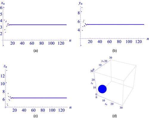
Here we will verify theoretical results obtain in Section 2–3 numerically. If ${\alpha }_{19}=45,{\beta }_{19}=4,{\gamma }_{19}=7.0,{\alpha }_{20}=39,{\beta }_{20}=3,{\gamma }_{20}=4,{\alpha }_{21}=59,{\beta }_{21}=2,{\gamma }_{21}=4$ then (3) with $x_0=0.2,x_{-1}=0.7,y_0=0.4,y_{-1}=1.9,z_0=0.4,z_{-1}=0.9$ can be written as (95) $\begin{array}{rl}{x}_{n+1}& =\frac{45+4e^{-y_n}}{7.0+z_{n-1}},y_{n+1}=\frac{39+3e^{-z_n}}{4+x_{n-1}},\\ z_{n+1}& =\frac{59+2e^{-x_n}}{48+y_{n-1}}.\end{array}$(95)

From computations it is easy to confirm that for above chosen values of parameters ${\alpha }_{19}=45,{\beta }_{19}=4,{\gamma }_{19}=7.0,{\alpha }_{20}=39,{\beta }_{20}=3,{\gamma }_{20}=4,{\alpha }_{21}=59,{\beta }_{21}=2,{\gamma }_{21}=4$ conditions under which ${\mathrm{\Gamma }}_1$ is globally asymptotically stable hold, i.e. $\begin{array}{rl}& {\beta }_{19}{\beta }_{20}{\beta }_{21}\\ & =24<{\gamma }_{19}{\gamma }_{20}{\gamma }_{21}=112\text{and}\\ & \frac{1}{{\gamma }_{19}+L_{21}}\left(\frac{{\beta }_{19}{e}^{-L_{20}}\left({\alpha }_{20}+{\beta }_{20}{e}^{-L_{21}}\right)}{{({\gamma }_{20}+L_{19})}^2}\right.\\ & \left.+\frac{{\beta }_{21}{e}^{-L_{19}}\left({\alpha }_{19}+{\beta }_{19}{e}^{-L_{20}}\right)}{\left({\gamma }_{19}+L_{21}\right)\left({\gamma }_{21}+L_{20}\right)}\right)\\ & +\frac{{\beta }_{20}{e}^{-L_{21}}\left({\alpha }_{21}+{\beta }_{21}{e}^{-L_{19}}\right)}{\left({\gamma }_{20}+L_{19}\right){({\gamma }_{21}+L_{20})}^2}\\ & +\frac{1}{\left({\gamma }_{19}+L_{21}\right)\left({\gamma }_{20}+L_{19}\right)\left({\gamma }_{21}+L_{20}\right)}.\end{array}$ $\begin{array}{rl}& \left(\frac{\begin{array}{c}{\beta }_{19}{\beta }_{20}{\beta }_{21}{e}^{-L_{19}-L_{20}-L_{21}}\\ +\left({\alpha }_{19}+{\beta }_{19}{e}^{-L_{20}}\right)\left({\alpha }_{20}+{\beta }_{20}{e}^{-L_{21}}\right)\\ \left({\alpha }_{21}+{\beta }_{21}{e}^{-L_{19}}\right)\end{array}}{\left({\gamma }_{19}+L_{21}\right)\left({\gamma }_{20}+L_{19}\right)\left({\gamma }_{21}+L_{20}\right)}\right)\\ & =0.0909986005619405595473877796<1.\end{array}$

Moreover, plot of $nvs{x}_n,nvs{y}_n,nvs{z}_n$ and its Global attractor is shown in Figure 1(a–d), respectively. Now if ${\alpha }_{19}=45,{\beta }_{19}=4,{\gamma }_{19}=27,{\alpha }_{20}=39,{\beta }_{20}=3,{\gamma }_{20}=14,{\alpha }_{21}=59,{\beta }_{21}=2,{\gamma }_{21}=4$ then (3) with $x_0=0.002,x_{-1}=0.07,y_0=0.004,y_{-1}=1.9,z_0=4,z_{-1}=0.9$ can be written as (96) $\begin{array}{rl}{x}_{n+1}& =\frac{45+4e^{-y_n}}{27+z_{n-1}},y_{n+1}=\frac{39+3e^{-z_n}}{14+x_{n-1}},\\ z_{n+1}& =\frac{59+2e^{-x_n}}{4+y_{n-1}}.\end{array}$(96) Computations show that if ${\alpha }_{19}=45,{\beta }_{19}=4,{\gamma }_{19}=27,{\alpha }_{20}=39,{\beta }_{20}=3,{\gamma }_{20}=14,{\alpha }_{21}=59,{\beta }_{21}=2,{\gamma }_{21}=4$ then conditions under which ${\mathrm{\Gamma }}_1$ is globally asymptotically stable hold, i.e. $\begin{array}{rl}{\beta }_{19}{\beta }_{20}{\beta }_{21}& =24<{\gamma }_{19}{\gamma }_{20}{\gamma }_{21}=1512\text{and}\frac{1}{{\gamma }_{19}+L_{21}}\\ & \times \left(\frac{{\beta }_{19}{e}^{-L_{20}}\left({\alpha }_{20}+{\beta }_{20}{e}^{-L_{21}}\right)}{{({\gamma }_{20}+L_{19})}^2}\right.\\ & \left.+\frac{{\beta }_{21}{e}^{-L_{19}}\left({\alpha }_{19}+{\beta }_{19}{e}^{-L_{20}}\right)}{\left({\gamma }_{19}+L_{21}\right)\left({\gamma }_{21}+L_{20}\right)}\right)\\ & +\frac{{\beta }_{20}{e}^{-L_{21}}\left({\alpha }_{21}+{\beta }_{21}{e}^{-L_{19}}\right)}{\left({\gamma }_{20}+L_{19}\right){({\gamma }_{21}+L_{20})}^2}\\ & +\frac{1}{\left({\gamma }_{19}+L_{21}\right)\left({\gamma }_{20}+L_{19}\right)\left({\gamma }_{21}+L_{20}\right)}.\end{array}$ $\begin{array}{rl}& \left(\begin{array}{c}{\beta }_{19}{\beta }_{20}{\beta }_{21}{e}^{-L_{19}-L_{20}-L_{21}}+\\ \frac{\left({\alpha }_{19}+{\beta }_{19}{e}^{-L_{20}}\right)\left({\alpha }_{20}+{\beta }_{20}{e}^{-L_{21}}\right)\left({\alpha }_{21}+{\beta }_{21}{e}^{-L_{19}}\right)}{\left({\gamma }_{19}+L_{21}\right)\left({\gamma }_{20}+L_{19}\right)\left({\gamma }_{21}+L_{20}\right)}\end{array}\right)\\ & =0.0856704522853635631846346627<1.\end{array}$

Figure 1. Graph for (95).

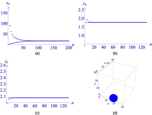
Moreover, plot of $nvs{x}_n,nvs{y}_n,nvs{z}_n$ and Global attractor is shown in Figure 2(a–d), respectively. For system (4), if we choose ${\alpha }_{22}=315,{\beta }_{22}=1.4,{\gamma }_{22}=1.7,{\alpha }_{23}=222,{\beta }_{23}=123,{\gamma }_{23}=124,{\alpha }_{24}=222,{\beta }_{24}=112,{\gamma }_{24}=114$ with $x_0=0.2,x_{-1}=0.1,y_0=0.4,y_{-1}=0.29,z_0=2,z_{-1}=0.9$ can be written as (97) $\begin{array}{rl}{x}_{n+1}& =\frac{315+1.4e^{-z_n}}{1.7+x_{n-1}},y_{n+1}=\frac{222+123e^{-x_n}}{124+y_{n-1}},\\ z_{n+1}& =\frac{222+1129e^{-y_n}}{114+z_{n-1}}.\end{array}$(97) For these values ${\alpha }_{22}=315,{\beta }_{22}=1.4,{\gamma }_{22}=1.7,{\alpha }_{23}=222,{\beta }_{23}=123,{\gamma }_{23}=124,{\alpha }_{24}=222,{\beta }_{24}=112,{\gamma }_{24}=114$ the conditions under which ${\mathrm{\Gamma }}_2$ is globally asymptotically stable satisfied, i.e. ${\beta }_{22}{\beta }_{23}{\beta }_{24}=19286.399999999998<{\gamma }_{22}{\gamma }_{23}{\gamma }_{24}=24031.199999999997$ and $\begin{array}{rl}& \frac{{\alpha }_{22}+{\beta }_{22}{e}^{-L_{24}}}{{({\gamma }_{22}+L_{22})}^2}\left(1+\frac{{\alpha }_{23}+{\beta }_{23}{e}^{-L_{22}}}{{({\gamma }_{23}+L_{23})}^2}\right)\\ & +\frac{{\alpha }_{23}+{\beta }_{23}{e}^{-L_{22}}}{{({\gamma }_{23}+L_{23})}^2}\left(1+\frac{{\alpha }_{24}+{\beta }_{24}{e}^{-L_{23}}}{{({\gamma }_{24}+L_{24})}^2}\right)\\ & +\frac{{\alpha }_{24}+{\beta }_{24}{e}^{-L_{23}}}{{({\gamma }_{24}+L_{24})}^2}\left(1+\frac{{\alpha }_{22}+{\beta }_{22}{e}^{-L_{24}}}{{({\gamma }_{22}+L_{22})}^2}\right)\\ & +\frac{1}{\left({\gamma }_{22}+L_{22}\right)\left({\gamma }_{23}+L_{23}\right)\left({\gamma }_{24}+L_{24}\right)}.\end{array}$ $\begin{array}{rl}& \left(\begin{array}{c}{\beta }_{22}{\beta }_{23}{\beta }_{24}{e}^{-L_{22}-L_{23}-L_{24}}+\\ \frac{\left({\alpha }_{22}+{\beta }_{22}{e}^{-L_{24}}\right)\left({\alpha }_{23}+{\beta }_{23}{e}^{-L_{22}}\right)\left({\alpha }_{24}+{\beta }_{24}{e}^{-L_{23}}\right)}{\left({\gamma }_{22}+L_{22}\right)\left({\gamma }_{23}+L_{23}\right)\left({\gamma }_{24}+L_{24}\right)}\end{array}\right)\\ & =0.2351437011808576519431082194520031<1.\end{array}$Moreover, plot of $nvs{x}_n,nvs{y}_n,nvs{z}_n$ and its attractor is shown in Figure 3(a–d), respectively.

Figure 2. Graph for (96).

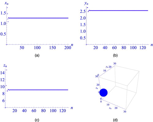
Figure 3. Graph for (97).

5. Conclusions

We have explored the global properties of exponential systems of difference equations. For both systems, we have studied the dynamics including boundedness and persistence, existence of invariant rectangle, existence of the unique $+\text{ve}$ equilibrium, global and local dynamics about the unique $+\text{ve}$ equilibrium point and conclusion are presented in Tables 2–4. Furthermore rate of convergence for each system is also demonstrated. Finally, theoretical results are verified numerically.

Table 2. Existence of invariant rectangle corresponding to system (3) and (4).

Systems	Existence of invariant rectangle
(3)	$\left[L_{19},U_{19}\right]\times [L_{20},U_{20}\left]\times \right[L_{21},U_{21}]$ where
	$L_{19}={\displaystyle \frac{{\alpha }_{19}+{\beta }_{19}{e}^{-{\displaystyle \frac{{\alpha }_{20}+{\beta }_{20}}{{\gamma }_{20}}}}}{{\gamma }_{19}+{\displaystyle \frac{{\alpha }_{21}+{\beta }_{21}}{{\gamma }_{21}}}}},U_{19}={\displaystyle \frac{{\alpha }_{19}+{\beta }_{19}}{{\gamma }_{19}}},L_{20}={\displaystyle \frac{{\alpha }_{20}+{\beta }_{20}{e}^{-{\displaystyle \frac{{\alpha }_{21}+{\beta }_{21}}{{\gamma }_{21}}}}}{{\gamma }_{20}+{\displaystyle \frac{{\alpha }_{19}+{\beta }_{19}}{{\gamma }_{19}}}}},U_{20}={\displaystyle \frac{{\alpha }_{20}+{\beta }_{20}}{{\gamma }_{20}}},$
	$L_{21}={\displaystyle \frac{{\alpha }_{21}+{\beta }_{21}{e}^{-{\displaystyle \frac{{\alpha }_{19}+{\beta }_{19}}{{\gamma }_{19}}}}}{{\gamma }_{21}+{\displaystyle \frac{{\alpha }_{20}+{\beta }_{20}}{{\gamma }_{20}}}}},U_{21}={\displaystyle \frac{{\alpha }_{21+}{\beta }_{21}}{{\gamma }_{21}}}.$
(4)	$[L_{22},U_{22}]\times [L_{23},U_{23}]\times [L_{24},U_{24}]$ where
	$L_{22}={\displaystyle \frac{{\alpha }_{22}+{\beta }_{22}{e}^{-{\displaystyle \frac{{\alpha }_{24}+{\beta }_{24}}{{\gamma }_{24}}}}}{{\gamma }_{22}+{\displaystyle \frac{{\alpha }_{22}+{\beta }_{22}}{{\gamma }_{22}}}}},U_{22}={\displaystyle \frac{{\alpha }_{22}+{\beta }_{22}}{{\gamma }_{22}}},L_{23}={\displaystyle \frac{{\alpha }_{23+}{\beta }_{23}{e}^{-{\displaystyle \frac{{\alpha }_{22}+{\beta }_{22}}{{\gamma }_{22}}}}}{{\gamma }_{23}+{\displaystyle \frac{{\alpha }_{23}+{\beta }_{23}}{{\gamma }_{23}}}}},U_{23}={\displaystyle \frac{{\alpha }_{23}+{\beta }_{23}}{{\gamma }_{23}}},$
	$L_{24}={\displaystyle \frac{{\alpha }_{24}+{\beta }_{24}{e}^{-{\displaystyle \frac{{\alpha }_{23}+{\beta }_{23}}{{\gamma }_{23}}}}}{{\gamma }_{24}+{\displaystyle \frac{{\alpha }_{24}+{\beta }_{24}}{{\gamma }_{24}}}}},U_{24}={\displaystyle \frac{{\alpha }_{24+}{\beta }_{24}}{{\gamma }_{24}}}.$

Table 3. Existence of the uniqueness $+\text{ve}$ equilibrium of system (3) and (4).

Systems	Existence of the uniqueness $+\text{ve}$ equilibrium
(3)	${\beta }_{19}{\beta }_{20}{\beta }_{21}<{\gamma }_{19}{\gamma }_{20}{\gamma }_{21}.$
(4)	${\beta }_{22}{\beta }_{23}{\beta }_{24}<{\gamma }_{22}{\gamma }_{23}{\gamma }_{24}.$

Table 4. Existence of parametric conditions under which the $+\text{ve}$ equilibrium of system (3) and (4) is globally asymptotically stable.

Systems	Existence of parametric conditions under which the $+\text{ve}$ equilibrium point is GAS
(3)	$\left(\overline{x},\overline{y},\overline{z}\right)\in \left[L_{19},U_{19}\right]\times [L_{20},U_{20}\left]\times \right[L_{21},U_{21}]$ is GAS if
	${\beta }_{19}{\beta }_{20}{\beta }_{21}<{\gamma }_{19}{\gamma }_{20}{\gamma }_{21}$ and
	${\displaystyle \frac{1}{{\gamma }_{19}+L_{21}}}\left({\displaystyle \frac{{\beta }_{19}{e}^{-L_{20}}\left({\alpha }_{20}+{\beta }_{20}{e}^{-L_{21}}\right)}{{({\gamma }_{20}+L_{19})}^2}}+{\displaystyle \frac{{\beta }_{21}{e}^{-L_{19}}\left({\alpha }_{19}+{\beta }_{19}{e}^{-L_{20}}\right)}{\left({\gamma }_{19}+L_{21}\right)\left({\gamma }_{21}+L_{20}\right)}}\right)+{\displaystyle \frac{{\beta }_{20}{e}^{-L_{21}}\left({\alpha }_{21}+{\beta }_{21}{e}^{-L_{19}}\right)}{\left({\gamma }_{20}+L_{19}\right){({\gamma }_{21}+L_{20})}^2}}+{\displaystyle \frac{1}{\left({\gamma }_{19}+L_{21}\right)\left({\gamma }_{20}+L_{19}\right)\left({\gamma }_{21}+L_{20}\right)}}\left(\begin{array}{c}{\beta }_{19}{\beta }_{20}{\beta }_{21}{e}^{-L_{19}-L_{20}-L_{21}}+\\ {\displaystyle \frac{\left({\alpha }_{19}+{\beta }_{19}{e}^{-L_{20}}\right)\left({\alpha }_{20}+{\beta }_{20}{e}^{-L_{21}}\right)\left({\alpha }_{21}+{\beta }_{21}{e}^{-L_{19}}\right)}{\left({\gamma }_{19}+L_{21}\right)\left({\gamma }_{20}+L_{19}\right)\left({\gamma }_{21}+L_{20}\right)}}\end{array}\right)<1.$
(4)	$\left(\overline{x},\overline{y},\overline{z}\right)\in \left[L_{22},U_{22}\right]\times [L_{23},U_{23}\left]\times \right[L_{24},U_{24}]$ is GAS if ${\beta }_{22}{\beta }_{23}{\beta }_{24}<{\gamma }_{22}{\gamma }_{23}{\gamma }_{24}$ and
	${\displaystyle \frac{{\alpha }_{22}+{\beta }_{22}{e}^{-L_{24}}}{{({\gamma }_{22}+L_{22})}^2}}\left(1+{\displaystyle \frac{{\alpha }_{23}+{\beta }_{23}{e}^{-L_{22}}}{{({\gamma }_{23}+L_{23})}^2}}\right)+{\displaystyle \frac{{\alpha }_{23}+{\beta }_{23}{e}^{-L_{22}}}{{({\gamma }_{23}+L_{23})}^2}}\left(1+{\displaystyle \frac{{\alpha }_{24}+{\beta }_{24}{e}^{-L_{23}}}{{({\gamma }_{24}+L_{24})}^2}}\right)+{\displaystyle \frac{{\alpha }_{24}+{\beta }_{24}{e}^{-L_{23}}}{{({\gamma }_{24}+L_{24})}^2}}\left(1+{\displaystyle \frac{{\alpha }_{22}+{\beta }_{22}{e}^{-L_{24}}}{{({\gamma }_{22}+L_{22})}^2}}\right)$
	$+{\displaystyle \frac{1}{\left({\gamma }_{22}+L_{22}\right)\left({\gamma }_{23}+L_{23}\right)\left({\gamma }_{24}+L_{24}\right)}}\left(\begin{array}{c}{\beta }_{22}{\beta }_{23}{\beta }_{24}{e}^{-L_{22}-L_{23}-L_{24}}+\\ {\displaystyle \frac{\left({\alpha }_{22}+{\beta }_{22}{e}^{-L_{24}}\right)\left({\alpha }_{23}+{\beta }_{23}{e}^{-L_{22}}\right)\left({\alpha }_{24}+{\beta }_{24}{e}^{-L_{23}}\right)}{\left({\gamma }_{22}+L_{22}\right)\left({\gamma }_{23}+L_{23}\right)\left({\gamma }_{24}+L_{24}\right)}}\end{array}\right)<1.$

Acknowledgement

The author declares that he got no funding on any part of this research.

Disclosure statement

No potential conflict of interest was reported by the author.

ORCID

A. Q. Khan http://orcid.org/0000-0002-0278-1352

References

- Ozturk I, Bozkurt F, Ozen S. On the difference equation: xn+1=(α1+α2e−xn)/α3+xn−1. Appl Math Comput. 2006;181:1387–1393.
- Papaschinopoulos G, Radin MA, Schinas CJ. Study of the asymptotic behavior of the solutions of three systems of difference equations of exponential form. Appl Math Comput. 2012;218:5310–5318.
- Grove EA, Ladas G. Periodicities in nonlinear difference equations. Boca Raton, FL: CRC Press; 2004.
- Kulenovic MRS, Ladas G. Dynamics of second-order rational difference equations. Boca Raton, FL: CRC Press; 2002.
- Sedaghat H. Nonlinear difference equations: theory with applications to social science models. Dordrecht: Kluwer Academic; 2003.
- Kalabusic S, Kulenovic MRS. Rate of convergence of solutions of rational difference equations of second-order. Adv Diff Eq. 2004;2:121–139.
- Pituk M. More on Poincare’s and Perron’s theorems for difference equations. J Diff Eq Appl. 2002;8:201–216.