Theory and application for the time fractional Gardner equation with Mittag-Leffler kernel

Abstract

In this work, the time fractional Gardner equation is presented as a new fractional model for Atangana–Baleanu fractional derivative with Mittag-Leffler kernel. The approximate consequences are analysed by applying a recurrent process. The existence and uniqueness of solution for this system is discussed. To explain the effects of several parameters and variables on the movement, the approximate results are shown in graphics and tables.

Keywords:

• The time fractional Gardner equation
• Atangana–Baleanu derivative
• Mittag-Leffler kernel
• existence and uniqueness
• series solution

1. Introduction

In the last few years, there has been considerable interest and significant theoretical developments in fractional calculus used in many fields and in fractional differential equations and its applications [1–7]. Abdeljawad and Baleanu [8] used discrete fractional differences with non-singular discrete Mittag-Leffler kernels; Owolabi and Atangana [9] investigated the mathematical analysis and numerical simulation of pattern formation in a subdiffusive multicomponent fractional-reaction diffusion system; in [10], Abdeljawad and Baleanu introduced non-local fractional derivative with Mittag-Leffler kernel; Abdeljawad [11] defined a Lyapunov type inequality for fractional operators with non-singular Mittag-Leffler kernel; Abdeljawad and Al-Mdallal studied the Caputo and Riemann–Liouville type discrete fractional in [12]; in [13], Abdeljawad and Madjidi investigated Lyapunov-type inequalities for fractional difference operators with discrete Mittag-Leffler kernel of order $2<\alpha <5/2;$ Zhang et al. [14] applied the series expansion process with local fractional operator to find the solutions of transport equations; Khan et al. investigated the advection–reaction diffusion model involving fractional-order derivatives with Mittag-Leffler kernel in [15]; Khan et al. [16] deal with two core aspects of fractional calculus in Caputo sense; Gómez-Aguilar et al. [17] considered three-dimensional cancer model using the Caputo–Fabrizio–Caputo type and with Mittag-Leffler kernel in Liouville–Caputo sense and Khan et al. [18] studied fractional order nonlinear Klein–Gordon equations with the help of the Sumudu decomposition method. Many more research studies related to fractional derivatives can be seen in [19–28].

In this study, we apply the fractional homotopy perturbation transform method (FHPTM) to find numerical solution for a fractional equation. The FHPTM is a combination of HPM and Laplace transform process [19–21]. Besides, the solution is in the form of a convergent series. An iterative process is composed for the shape of the infinite numerical solution. In [22], Kumar et al. analysed the numerical solution for fractional RLW equation by using this method, and, in [23], this method is used to find the series solutions of logarithmic KdV equation.

In this work, we analysed the time fractional Gardner equation (FGE). The Gardner equation is an advantageous example for the definition of interior solitary waves in shallow water , while Buckmaster's equation is applied in thin viscous fluid sheet flows and has been generally examined by several methods (see [24–26]).

This equation is given by [26], $\begin{array}{rl}& D_{\tau }^{\alpha }p(\varkappa ,\tau )+6\left(p\right(\varkappa ,\tau )-{\epsilon }^{2}p(\varkappa ,\tau {)}^2\left)p_{\varkappa }\right(\varkappa ,\tau )\\ & +p_{\varkappa \varkappa \varkappa }(\varkappa ,\tau )=0,\\ & \varkappa \in R,\tau >0,0<\alpha \le 1,\end{array}$ with the primary situation $p(\varkappa ,0)=\frac{1}{2}+\frac{1}{2}\tanh \frac{\varkappa }{2}.$ The analytical solution to this model, for $\epsilon =1$ and $\alpha =1$, is $p(\varkappa ,\tau )=\frac{1}{2}+\frac{1}{2}\tanh \frac{\varkappa -\tau }{2}.$ Some fractional derivatives contain singular kernels. Two of them are Riemann and Caputo and they have their own restrictions due to their singular kernels. However, recently some fractional operators such as Atangana–Baleanu (AB) have defeated these restrictions and deficiencies. In particular, AB used a new fractional derivative with non-singular, non-local and ML kernel and cleared its significant effects [27,29]. In [30], Yadav et al. investigated numerical schemes to compute ABC derivative; Chatibi et al. applied variational calculus involving non-local fractional derivative with Mittag-Leffler kernel in [31] and Koca obtained numerical solutions the fractional partial differential equations with non-singular kernel derivatives in [32].

We analyse FGE for AB fractional operator with Mittag-Leffler kernel due to the great importance of AB fractional derivative in scientific and engineering fields.

The FGE with AB fractional derivative is given as $\begin{array}{rl}& {}_a^{ABC}{D}_{\tau }^{\alpha }p(\varkappa ,\tau )+6\left(p\right(\varkappa ,\tau )-{\epsilon }^{2}p(\varkappa ,\tau {)}^2\left)p_{\varkappa }\right(\varkappa ,\tau )\\ & +p_{\varkappa \varkappa \varkappa }(\varkappa ,\tau )=0,0<\alpha \le 1.\end{array}$

The main purpose of this article is to analyse FGE with Mittag-Leffler kernel. The existence and uniqueness analysis of the solutions for FGE has been viewed by using the fixed-point theorem.

In Section 2 of this study, various basic knowledge regarding the AB fractional order derivative are defined. In the next section, FGE with AB fractional derivative is investigated and the existence and uniqueness of solutions for these systems has been investigated by using the fixed-point theorem. In the next section, the FHPTM is applied to construct the solutions of the FGE for AB fractional derivative with Mittag-Leffler kernel. In Section 5, some graphical representations of the solutions are shown to display the accuracy and efficiency of the method. Moreover, some results are pointed out in Section 6.

2. Preliminaries

In this part, we will present the basic definitions and several properties for AB fractional order derivative [8,28,29,33–35].

Definition 2.1

When $p\in H^1(\varkappa ,y),\alpha \in [0,1],$ $y>\varkappa$ and differentiable, AB fractional order derivative with arbitrary order in the case of Caputo is given as (2.1) $\begin{array}{rl}& {}_a^{ABC}{D}_{\tau }^{\alpha }\left(p\right(\tau \left)\right)\\ & =\frac{B\left(\alpha \right)}{1-\alpha }{\int }_{\varkappa }^{\tau }{p}^{\mathrm{\prime }}\left(s\right)E_{\alpha }\left[-\frac{\alpha }{1-\alpha }(\tau -s{)}^{\alpha }\right]\mathrm{d}s,\end{array}$(2.1) where $B\left(\alpha \right)$ provides the requirement $B\left(0\right)=B\left(1\right)=1$.

Definition 2.2

When $p\in H^1(\varkappa ,y),\alpha \in [0,1],$ $y>\varkappa$ and is not necessarily differentiable, the AB derivative of arbitrary order in the case of Riemann–Liouville is given as (2.2) $\begin{array}{rl}& {}_a^{ABR}{D}_{\tau }^{\alpha }\left(p\right(\tau \left)\right)\\ & =\frac{B\left(\alpha \right)}{1-\alpha }\frac{\mathrm{d}}{\mathrm{d}\tau }{\int }_{\varkappa }^{\tau }p\left(s\right)E_{\alpha }\left[-\frac{\alpha }{1-\alpha }(\tau -s{)}^{\alpha }\right]\mathrm{d}s.\end{array}$(2.2)

Definition 2.3

When $0<\alpha <1$, and $p=p\left(\tau \right)$, the fractional integral operator of order α is given as [8] (2.3) $\begin{array}{rl}& {}_a^{ABR}{I}_{\tau }^{\alpha }\left(p\right(\tau \left)\right)\\ & =\frac{1-\alpha }{B\left(\alpha \right)}p\left(\tau \right)+\frac{\alpha }{B\left(\alpha \right)\mathrm{\Gamma }\left(\alpha \right)}{\int }_{\varkappa }^{\tau }p\left(l\right)(\tau -l{)}^{\alpha -1}\mathrm{d}l.\end{array}$(2.3)

3. Analysis of the FGE with AB fractional derivative

The FGE is written as: $0<\alpha <1,$ (3.1) $\begin{array}{rl}& {}_a^{ABC}{D}_{\tau }^{\alpha }p(\varkappa ,\tau )+6\left(p\right(\varkappa ,\tau )-{\epsilon }^{2}p(\varkappa ,\tau {)}^2\left)p_{\varkappa }\right(\varkappa ,\tau )\\ & +p_{\varkappa \varkappa \varkappa }(\varkappa ,\tau )=0,\end{array}$(3.1) with the initial condition $p(\varkappa ,0)=\frac{1}{2}+\frac{1}{2}\tanh \left(\frac{\varkappa }{2}\right).$ Using the fractional integral operator produced by AB [8,35] in Equation (3.1(3.1) $\begin{array}{rl}& {}_a^{ABC}{D}_{\tau }^{\alpha }p(\varkappa ,\tau )+6\left(p\right(\varkappa ,\tau )-{\epsilon }^{2}p(\varkappa ,\tau {)}^2\left)p_{\varkappa }\right(\varkappa ,\tau )\\ & +p_{\varkappa \varkappa \varkappa }(\varkappa ,\tau )=0,\end{array}$(3.1) ), we obtain (3.2) $\begin{array}{rl}& p(\varkappa ,\tau )-p(\varkappa ,0)\\ & =\frac{1-\alpha }{B\left(\alpha \right)}K(\varkappa ,\tau ,p)\\ & +\frac{\alpha }{B\left(\alpha \right)\mathrm{\Gamma }\left(\alpha \right)}{\int }_0^{\tau }(\tau -l{)}^{\alpha -1}K(\varkappa ,l,p)\mathrm{d}l,\end{array}$(3.2) where $\begin{array}{rl}K(\varkappa ,\tau ,p)& =-6\left(p\right(\varkappa ,\tau )-{\epsilon }^{2}p(\varkappa ,\tau {)}^2\left)p_{\varkappa }\right(\varkappa ,\tau )\\ & -p_{\varkappa \varkappa \varkappa }(\varkappa ,\tau )\\ & =-6p(\varkappa ,\tau )p_{\varkappa }(\varkappa ,\tau )+6{\epsilon }^{2}p(\varkappa ,\tau {)}^2{p}_{\varkappa }(\varkappa ,\tau )\\ & -p_{\varkappa \varkappa \varkappa }(\varkappa ,\tau ).\end{array}$

The kernel $K(\varkappa ,\tau ,p)$ has the Lipschitz state, which justified that the function $p(\varkappa ,\tau )$ has upper bound. So, (3.3) $\begin{array}{rl}& ∥K(\varkappa ,\tau ,p)-K(\varkappa ,\tau ,P)∥\\ & =∥-6\left(p{p}_{\varkappa }-P{P}_{\varkappa }\right)+6{\epsilon }^2\left(p^2{p}_{\varkappa }-P^2{P}_{\varkappa }\right)\\ & -\left(p_{\varkappa \varkappa \varkappa }-P_{\varkappa \varkappa \varkappa }\right)\phantom{6{\epsilon }^2}∥.\end{array}$(3.3) By applying the triangular inequality of norm in Equation (3.3(3.3) $\begin{array}{rl}& ∥K(\varkappa ,\tau ,p)-K(\varkappa ,\tau ,P)∥\\ & =∥-6\left(p{p}_{\varkappa }-P{P}_{\varkappa }\right)+6{\epsilon }^2\left(p^2{p}_{\varkappa }-P^2{P}_{\varkappa }\right)\\ & -\left(p_{\varkappa \varkappa \varkappa }-P_{\varkappa \varkappa \varkappa }\right)\phantom{6{\epsilon }^2}∥.\end{array}$(3.3) ), (3.4) $\begin{array}{rl}& ∥K(\varkappa ,\tau ,p)-K(\varkappa ,\tau ,P)∥\\ & \le -6∥p{p}_{\varkappa }-P{P}_{\varkappa }∥+6{\epsilon }^2∥p^2{p}_{\varkappa }-P^2{P}_{\varkappa }∥\\ & -∥p_{\varkappa \varkappa \varkappa }-P_{\varkappa \varkappa \varkappa }∥\\ & \le -3∥\frac{\mathrm{\partial }}{\mathrm{\partial }\varkappa }(p^2-P^2)∥+2{\epsilon }^2∥\frac{\mathrm{\partial }}{\mathrm{\partial }\varkappa }(p^3-P^3)∥\\ & -∥\frac{{\mathrm{\partial }}^3}{\mathrm{\partial }{\varkappa }^3}(p-P)∥\\ & \le -3\delta (a+b)∥p-P∥\\ & +2{\epsilon }^2\gamma (a^2+ab+b^2)∥p-P∥-{\kappa }^3∥p-P∥\\ & \le (-3\delta (a+b)+2{\epsilon }^2\gamma (a^2+ab+b^2)-{\kappa }^3)\\ & \times ∥p-P∥.\end{array}$(3.4) Setting $\mathrm{\Phi }=-3\delta (a+b)+2{\epsilon }^2\gamma (a^2+ab+b^2)-{\kappa }^3,$ where p and P are limited functions, we can say $\parallel p\parallel \le a,\parallel P\parallel \le b$ and we have $∥K(\varkappa ,\tau ,p)-K(\varkappa ,\tau ,P)∥\le \mathrm{\Phi }∥p-P∥.$ Then, the Lipschitz state is justified for the kernel $K(\varkappa ,\tau ,p).$

3.1. Existence and uniqueness analysis for solutions

In this part, we will present the existence and uniqueness of the solution of FGE for arbitrary order (3.1(3.1) $\begin{array}{rl}& {}_a^{ABC}{D}_{\tau }^{\alpha }p(\varkappa ,\tau )+6\left(p\right(\varkappa ,\tau )-{\epsilon }^{2}p(\varkappa ,\tau {)}^2\left)p_{\varkappa }\right(\varkappa ,\tau )\\ & +p_{\varkappa \varkappa \varkappa }(\varkappa ,\tau )=0,\end{array}$(3.1) ). From Equation (3.2(3.2) $\begin{array}{rl}& p(\varkappa ,\tau )-p(\varkappa ,0)\\ & =\frac{1-\alpha }{B\left(\alpha \right)}K(\varkappa ,\tau ,p)\\ & +\frac{\alpha }{B\left(\alpha \right)\mathrm{\Gamma }\left(\alpha \right)}{\int }_0^{\tau }(\tau -l{)}^{\alpha -1}K(\varkappa ,l,p)\mathrm{d}l,\end{array}$(3.2) ), we have (3.5) $\begin{array}{rl}{p}_{n+1}(\varkappa ,\tau )& =\frac{1-\alpha }{B\left(\alpha \right)}K(\varkappa ,\tau ,p_n)\\ & +\frac{\alpha }{B\left(\alpha \right)\mathrm{\Gamma }\left(\alpha \right)}{\int }_0^{\tau }(\tau -l{)}^{\alpha -1}K(\varkappa ,l,p_n)\mathrm{d}l,\end{array}$(3.5) and $p_0(\varkappa ,\tau )=p(\varkappa ,0).$

The difference of the successive terms is represented as follows: (3.6) $\begin{array}{rl}{Y}_n(\varkappa ,\tau )& =p_n(\varkappa ,\tau )-p_{n-1}(\varkappa ,\tau )\\ & =\frac{1-\alpha }{B\left(\alpha \right)}\left\{K\right(\varkappa ,\tau ,p_{n-1})\\ & -K(\varkappa ,\tau ,p_{n-2})\}+\frac{\alpha }{B\left(\alpha \right)\mathrm{\Gamma }\left(\alpha \right)}\\ & \times {\int }_0^{\tau }(\tau -l{)}^{\alpha -1}\{K(\varkappa ,l,p_{n-1})\\ & -K(\varkappa ,l,p_{n-2})\}\mathrm{d}l,\end{array}$(3.6) where we say that, (3.7) $p_n(\varkappa ,\tau )=\sum _{k=0}^n{Y}_k(\varkappa ,\tau ).$(3.7) From Equation (3.7(3.7) $p_n(\varkappa ,\tau )=\sum _{k=0}^n{Y}_k(\varkappa ,\tau ).$(3.7) ), we get (3.8) $\begin{array}{rl}& ∥Y_n(\varkappa ,\tau )∥\\ & =∥p_n(\varkappa ,\tau )-p_{n-1}(\varkappa ,\tau )∥\\ & =∥\begin{array}{c}\frac{1-\alpha }{B\left(\alpha \right)}\left\{K\right(\varkappa ,\tau ,p_{n-1})-K(\varkappa ,\tau ,p_{n-2}\left)\right\}\\ +\frac{\alpha }{B\left(\alpha \right)\mathrm{\Gamma }\left(\alpha \right)}{\int }_0^{\tau }(\tau -l{)}^{\alpha -1}\{K(\varkappa ,l,p_{n-1})\\ -K(\varkappa ,l,p_{n-2})\}\mathrm{d}l\end{array}∥\end{array}$(3.8) Using the triangular inequality in Equation (3.8(3.8) $\begin{array}{rl}& ∥Y_n(\varkappa ,\tau )∥\\ & =∥p_n(\varkappa ,\tau )-p_{n-1}(\varkappa ,\tau )∥\\ & =∥\begin{array}{c}\frac{1-\alpha }{B\left(\alpha \right)}\left\{K\right(\varkappa ,\tau ,p_{n-1})-K(\varkappa ,\tau ,p_{n-2}\left)\right\}\\ +\frac{\alpha }{B\left(\alpha \right)\mathrm{\Gamma }\left(\alpha \right)}{\int }_0^{\tau }(\tau -l{)}^{\alpha -1}\{K(\varkappa ,l,p_{n-1})\\ -K(\varkappa ,l,p_{n-2})\}\mathrm{d}l\end{array}∥\end{array}$(3.8) ), we have (3.9) $\begin{array}{rl}& ∥Y_n(\varkappa ,\tau )∥\\ & \le \begin{array}{c}\frac{1-\alpha }{B\left(\alpha \right)}∥K(\varkappa ,\tau ,p_{n-1})-K(\varkappa ,\tau ,p_{n-2})∥\\ +\frac{\alpha }{B\left(\alpha \right)\mathrm{\Gamma }\left(\alpha \right)}{\int }_0^{\tau }(\tau -l{)}^{\alpha -1}∥\begin{array}{c}K(\varkappa ,l,p_{n-1})\\ -K(\varkappa ,l,p_{n-2})\end{array}∥\mathrm{d}l.\end{array}\end{array}$(3.9) As the kernel justifies the Lipschitz state, they give (3.10) $\begin{array}{rl}∥Y_n(\varkappa ,\tau )∥& \le \frac{1-\alpha }{B\left(\alpha \right)}\mathrm{\Phi }∥p_{n-1}-p_{n-2}∥+\frac{\alpha }{B\left(\alpha \right)\mathrm{\Gamma }\left(\alpha \right)}\\ & \times {\int }_0^{\tau }(\tau -l{)}^{\alpha -1}\mathrm{\Phi }∥p_{n-1}-p_{n-2}∥\mathrm{d}l,\end{array}$(3.10) or (3.11) $\begin{array}{rl}∥Y_n(\varkappa ,\tau )∥& \le \frac{1-\alpha }{B\left(\alpha \right)}\mathrm{\Phi }∥Y_{n-1}(\varkappa ,\tau )∥+\frac{\alpha }{B\left(\alpha \right)\mathrm{\Gamma }\left(\alpha \right)}\\ & \times \mathrm{\Phi }{\int }_0^{\tau }(\tau -l{)}^{\alpha -1}∥Y_{n-1}(\varkappa ,\tau )∥\mathrm{d}l.\end{array}$(3.11)

Theorem 3.1

The FGE given as Equation (3.1(3.1) $\begin{array}{rl}& {}_a^{ABC}{D}_{\tau }^{\alpha }p(\varkappa ,\tau )+6\left(p\right(\varkappa ,\tau )-{\epsilon }^{2}p(\varkappa ,\tau {)}^2\left)p_{\varkappa }\right(\varkappa ,\tau )\\ & +p_{\varkappa \varkappa \varkappa }(\varkappa ,\tau )=0,\end{array}$(3.1) ) has the solutions that provide the following conditions that is found with ${\xi }_0$: (3.12) $\frac{1-\alpha }{B\left(\alpha \right)}\mathrm{\Phi }+\frac{\alpha }{B\left(\alpha \right)\mathrm{\Gamma }\left(\alpha \right)}\mathrm{\Phi }{\xi }_0^{\alpha }<1.$(3.12)

Proof.

Let us consider that the function $p(\varkappa ,\tau )$ is limited. Additionally, it has already been stated that the kernel provides the Lipschitz state; hence, from Equation (3.12(3.12) $\frac{1-\alpha }{B\left(\alpha \right)}\mathrm{\Phi }+\frac{\alpha }{B\left(\alpha \right)\mathrm{\Gamma }\left(\alpha \right)}\mathrm{\Phi }{\xi }_0^{\alpha }<1.$(3.12) ), Equation (3.11(3.11) $\begin{array}{rl}∥Y_n(\varkappa ,\tau )∥& \le \frac{1-\alpha }{B\left(\alpha \right)}\mathrm{\Phi }∥Y_{n-1}(\varkappa ,\tau )∥+\frac{\alpha }{B\left(\alpha \right)\mathrm{\Gamma }\left(\alpha \right)}\\ & \times \mathrm{\Phi }{\int }_0^{\tau }(\tau -l{)}^{\alpha -1}∥Y_{n-1}(\varkappa ,\tau )∥\mathrm{d}l.\end{array}$(3.11) ) is written as follows: (3.13) $∥Y_n(\varkappa ,\tau )∥\le {\left[\frac{1-\alpha }{B\left(\alpha \right)}\mathrm{\Phi }+\frac{\alpha }{B\left(\alpha \right)\mathrm{\Gamma }\left(\alpha \right)}\mathrm{\Phi }{\xi }^{\alpha }\right]}^n∥p(\varkappa ,0)∥$(3.13) Therefore, the function (3.14) $p_n(\varkappa ,\tau )=\sum _{k=0}^n{Y}_k(\varkappa ,\tau )$(3.14) exists and is smooth. Now, we examine that the function given in the above equation is the solution of Equation (3.1(3.1) $\begin{array}{rl}& {}_a^{ABC}{D}_{\tau }^{\alpha }p(\varkappa ,\tau )+6\left(p\right(\varkappa ,\tau )-{\epsilon }^{2}p(\varkappa ,\tau {)}^2\left)p_{\varkappa }\right(\varkappa ,\tau )\\ & +p_{\varkappa \varkappa \varkappa }(\varkappa ,\tau )=0,\end{array}$(3.1) ). Let us consider $p(\varkappa ,\tau )-p(\varkappa ,0)=p_n(\varkappa ,\tau )-D_n(\varkappa ,\tau ).$ Therefore, we have (3.15) $\begin{array}{rl}∥D_n(\varkappa ,\tau )∥& =∥\begin{array}{c}\frac{1-\alpha }{B\left(\alpha \right)}\left[K(\varkappa ,\tau ,p)-K(\varkappa ,\tau ,p_{n-1})\right]\\ +\frac{\alpha }{B\left(\alpha \right)\mathrm{\Gamma }\left(\alpha \right)}{\int }_0^{\tau }(\tau -l{)}^{\alpha -1}\\ \left[\begin{array}{c}K(\varkappa ,l,p)\\ -K(\varkappa ,l,p_{n-1})\end{array}\right]\mathrm{d}l\end{array}∥\\ & \le \frac{1-\alpha }{B\left(\alpha \right)}∥K(\varkappa ,\tau ,p)-K(\varkappa ,\tau ,p_{n-1})∥\\ & +\frac{\alpha }{B\left(\alpha \right)\mathrm{\Gamma }\left(\alpha \right)}{\int }_0^{\tau }(\tau -l{)}^{\alpha -1}\\ & \times ∥\begin{array}{c}K(\varkappa ,l,p)\\ -K(\varkappa ,l,p_{n-1})\end{array}∥\mathrm{d}l\\ & \le \frac{1-\alpha }{B\left(\alpha \right)}\mathrm{\Phi }∥p-p_{n-1}∥\\ & +\frac{1}{B\left(\alpha \right)\mathrm{\Gamma }\left(\alpha \right)}\mathrm{\Phi }∥p-p_{n-1}∥{\xi }^{\alpha }.\end{array}$(3.15)

By continuing the same process, we have $∥D_n(\varkappa ,\tau )∥\le {\left(\frac{1-\alpha }{B\left(\alpha \right)}+\frac{1}{B\left(\alpha \right)\mathrm{\Gamma }\left(\alpha \right)}{\xi }^{\alpha }\right)}^{n+1}{\mathrm{\Phi }}^{n+1}d.$ Then, at $\xi ={\xi }_0,$ we have $∥D_n(\varkappa ,\tau )∥\le {\left(\frac{1-\alpha }{B\left(\alpha \right)}+\frac{1}{B\left(\alpha \right)\mathrm{\Gamma }\left(\alpha \right)}{\xi }_0^{\alpha }\right)}^{n+1}{\mathrm{\Phi }}^{n+1}d,$ where when $n\to \mathrm{\infty }$, we have $∥D_n(\varkappa ,\tau )∥\to 0.$ Then, the proof of existence is completed.

Now, we analyse the uniqueness of solution for FGE (3.1(3.1) $\begin{array}{rl}& {}_a^{ABC}{D}_{\tau }^{\alpha }p(\varkappa ,\tau )+6\left(p\right(\varkappa ,\tau )-{\epsilon }^{2}p(\varkappa ,\tau {)}^2\left)p_{\varkappa }\right(\varkappa ,\tau )\\ & +p_{\varkappa \varkappa \varkappa }(\varkappa ,\tau )=0,\end{array}$(3.1) ). Let us assume that $p(\varkappa ,\tau )$ gets another solution for Equation (3.1(3.1) $\begin{array}{rl}& {}_a^{ABC}{D}_{\tau }^{\alpha }p(\varkappa ,\tau )+6\left(p\right(\varkappa ,\tau )-{\epsilon }^{2}p(\varkappa ,\tau {)}^2\left)p_{\varkappa }\right(\varkappa ,\tau )\\ & +p_{\varkappa \varkappa \varkappa }(\varkappa ,\tau )=0,\end{array}$(3.1) ), (3.16) $\begin{array}{rl}& p(\varkappa ,\tau )-P(\varkappa ,\tau )\\ & =\frac{1-\alpha }{B\left(\alpha \right)}\left\{K(\varkappa ,\tau ,p)-K(\varkappa ,\tau ,P)\right\}\\ & +\frac{\alpha }{B\left(\alpha \right)\mathrm{\Gamma }\left(\alpha \right)}{\int }_0^{\tau }(\tau -l{)}^{\alpha -1}\left\{\begin{array}{c}K(\varkappa ,l,p)\\ -K(\varkappa ,l,P)\end{array}\right\}\mathrm{d}l.\end{array}$(3.16) Taking the norm on Equation (3.18(3.16) $\begin{array}{rl}& p(\varkappa ,\tau )-P(\varkappa ,\tau )\\ & =\frac{1-\alpha }{B\left(\alpha \right)}\left\{K(\varkappa ,\tau ,p)-K(\varkappa ,\tau ,P)\right\}\\ & +\frac{\alpha }{B\left(\alpha \right)\mathrm{\Gamma }\left(\alpha \right)}{\int }_0^{\tau }(\tau -l{)}^{\alpha -1}\left\{\begin{array}{c}K(\varkappa ,l,p)\\ -K(\varkappa ,l,P)\end{array}\right\}\mathrm{d}l.\end{array}$(3.16) ) gives $\begin{array}{rl}& ∥p(\varkappa ,\tau )-P(\varkappa ,\tau )∥\\ & \le \frac{1-\alpha }{B\left(\alpha \right)}∥K(\varkappa ,\tau ,p)-K(\varkappa ,\tau ,P)∥\\ & +\frac{\alpha }{B\left(\alpha \right)\mathrm{\Gamma }\left(\alpha \right)}{\int }_0^{\tau }(\tau -l{)}^{\alpha -1}∥\begin{array}{c}K(\varkappa ,l,p)\\ -K(\varkappa ,l,P)\end{array}∥\mathrm{d}l.\end{array}$ Since the kernel justifies the Lipschitz states, we have (3.17) $\begin{array}{rl}& ∥p(\varkappa ,\tau )-P(\varkappa ,\tau )∥\\ & \le \frac{1-\alpha }{B\left(\alpha \right)}\mathrm{\Phi }∥p(\varkappa ,\tau )-P(\varkappa ,\tau )∥\\ & +\frac{1}{B\left(\alpha \right)\mathrm{\Gamma }\left(\alpha \right)}\mathrm{\Phi }{\xi }^{\alpha }∥p(\varkappa ,\tau )-P(\varkappa ,\tau )∥.\end{array}$(3.17) This gives (3.18) $\begin{array}{rl}& ∥p(\varkappa ,\tau )-P(\varkappa ,\tau )∥\\ & \times \left(1-\frac{1-\alpha }{B\left(\alpha \right)}\mathrm{\Phi }-\frac{1}{B\left(\alpha \right)\mathrm{\Gamma }\left(\alpha \right)}\mathrm{\Phi }{\xi }^{\alpha }\right)\le 0.\end{array}$(3.18)

Theorem 3.2

If the following inequality is provided, there is a unique solution of FGE (3.1(3.1) $\begin{array}{rl}& {}_a^{ABC}{D}_{\tau }^{\alpha }p(\varkappa ,\tau )+6\left(p\right(\varkappa ,\tau )-{\epsilon }^{2}p(\varkappa ,\tau {)}^2\left)p_{\varkappa }\right(\varkappa ,\tau )\\ & +p_{\varkappa \varkappa \varkappa }(\varkappa ,\tau )=0,\end{array}$(3.1) ), (3.19) $\left(1-\frac{1-\alpha }{B\left(\alpha \right)}\mathrm{\Phi }-\frac{1}{B\left(\alpha \right)\mathrm{\Gamma }\left(\alpha \right)}\mathrm{\Phi }{\xi }^{\alpha }\right)>0.$(3.19)

Proof.

If the (3.19) condition is satisfied, then (3.20) $\begin{array}{rl}& ∥p(\varkappa ,\tau )-P(\varkappa ,\tau )∥\\ & \times \left(1-\frac{1-\alpha }{B\left(\alpha \right)}\mathrm{\Phi }-\frac{1}{B\left(\alpha \right)\mathrm{\Gamma }\left(\alpha \right)}\mathrm{\Phi }{\xi }^{\alpha }\right)\le 0\end{array}$(3.20) implies that $∥p(\varkappa ,\tau )-P(\varkappa ,\tau )∥=0.$ Then, we get $p(\varkappa ,\tau )=P(\varkappa ,\tau ).$ It completes the proof of the uniqueness of the solution for Equation (3.1(3.1) $\begin{array}{rl}& {}_a^{ABC}{D}_{\tau }^{\alpha }p(\varkappa ,\tau )+6\left(p\right(\varkappa ,\tau )-{\epsilon }^{2}p(\varkappa ,\tau {)}^2\left)p_{\varkappa }\right(\varkappa ,\tau )\\ & +p_{\varkappa \varkappa \varkappa }(\varkappa ,\tau )=0,\end{array}$(3.1) ).

4. FHPTM for the time fractional Gardner equation with AB fractional derivative

In this part, first of all, we consider the Laplace transform for FGE with AB fractional operator (3.1(3.1) $\begin{array}{rl}& {}_a^{ABC}{D}_{\tau }^{\alpha }p(\varkappa ,\tau )+6\left(p\right(\varkappa ,\tau )-{\epsilon }^{2}p(\varkappa ,\tau {)}^2\left)p_{\varkappa }\right(\varkappa ,\tau )\\ & +p_{\varkappa \varkappa \varkappa }(\varkappa ,\tau )=0,\end{array}$(3.1) ) by using FHPTM and use the following initial condition: $p(\varkappa ,0)=\frac{1}{2}\left(1+\tanh \left(\frac{\varkappa }{2}\right)\right),$ which yields (4.1) $\begin{array}{rl}L\left[p\right(\varkappa ,\tau \left)\right]& =\frac{\frac{1}{2}\left(1+\tanh \left(\frac{\varkappa }{2}\right)\right)}{s}-\left(\frac{s^{\alpha }+\alpha (1-s^{\alpha })}{s^{\alpha }}\right)\\ & L[-6p{p}_{\varkappa }+6{\epsilon }^2{p}^2{p}_{\varkappa }-p_{\varkappa \varkappa \varkappa }].\end{array}$(4.1) By using the inverse of Laplace transform in Equation (4.1(4.1) $\begin{array}{rl}L\left[p\right(\varkappa ,\tau \left)\right]& =\frac{\frac{1}{2}\left(1+\tanh \left(\frac{\varkappa }{2}\right)\right)}{s}-\left(\frac{s^{\alpha }+\alpha (1-s^{\alpha })}{s^{\alpha }}\right)\\ & L[-6p{p}_{\varkappa }+6{\epsilon }^2{p}^2{p}_{\varkappa }-p_{\varkappa \varkappa \varkappa }].\end{array}$(4.1) ), we have (4.2) $\begin{array}{rl}p(\varkappa ,\tau )& =\frac{1}{2}\left(1+\tanh \left(\frac{\varkappa }{2}\right)\right)-L^{-1}\\ & \times \left[\begin{array}{c}\left(\frac{s^{\alpha }+\alpha (1-s^{\alpha })}{s^{\alpha }}\right)\\ L\left[-6p{p}_{\varkappa }+6{\epsilon }^2{p}^2{p}_{\varkappa }-p_{\varkappa \varkappa \varkappa }\right]\end{array}\right],\end{array}$(4.2) by applying the HPM, we have (4.3) $\begin{array}{rl}\sum _{n=0}^{\mathrm{\infty }}{z}^n{p}_n& =\frac{1}{2}\left(1+\tanh \left(\frac{\varkappa }{2}\right)\right)\\ & -z\left(L^{-1}\left[\left(\frac{s^{\alpha }+\alpha (1-s^{\alpha })}{s^{\alpha }}\right)\right.\right.\\ & \times L\left[-6\sum _{n=0}^{\mathrm{\infty }}{z}^n{H}_n\left(p\right)\right.\\ & +\left.\left.\left.6{\epsilon }^2\sum _{n=0}^{\mathrm{\infty }}{z}^n{K}_n\left(p\right)-\sum _{n=0}^{\mathrm{\infty }}{z}^n{p}_{\varkappa \varkappa \varkappa }\right]\right]\right).\end{array}$(4.3) In Equation (4.3(4.3) $\begin{array}{rl}\sum _{n=0}^{\mathrm{\infty }}{z}^n{p}_n& =\frac{1}{2}\left(1+\tanh \left(\frac{\varkappa }{2}\right)\right)\\ & -z\left(L^{-1}\left[\left(\frac{s^{\alpha }+\alpha (1-s^{\alpha })}{s^{\alpha }}\right)\right.\right.\\ & \times L\left[-6\sum _{n=0}^{\mathrm{\infty }}{z}^n{H}_n\left(p\right)\right.\\ & +\left.\left.\left.6{\epsilon }^2\sum _{n=0}^{\mathrm{\infty }}{z}^n{K}_n\left(p\right)-\sum _{n=0}^{\mathrm{\infty }}{z}^n{p}_{\varkappa \varkappa \varkappa }\right]\right]\right).\end{array}$(4.3) ), $H_n\left(p\right)$ and $K_n\left(p\right)$ are He's polynomials as follows: $\sum _{n=0}^{\mathrm{\infty }}{z}^n{H}_n\left(p\right)=p{p}_{\varkappa },\sum _{n=0}^{\mathrm{\infty }}{z}^n{K}_n(p,q)=p^2{p}_{\varkappa }.$ The initial elements of the He's polynomials are described as $\begin{array}{rl}{H}_0\left(p\right)& =p_0{p}_{0_{\varkappa }},\\ H_1\left(p\right)& =p_0{p}_{1_{\varkappa }}+p_1{p}_{0_{\varkappa }},\\ H_2\left(p\right)& =p_0{p}_{2_{\varkappa }}+p_1{p}_{1_{\varkappa }}+p_2{p}_{0_{\varkappa }},\\ & ⋮\\ K_0\left(p\right)& =p_0^2{p}_{0_{\varkappa }},\\ K_1\left(p\right)& =p_0^2{p}_{1_{\varkappa }}+2p_0{p}_1{p}_{0_{\varkappa }},\\ K_2\left(p\right)& =p_0^2{p}_{2_{\varkappa }}+2p_0{p}_1{p}_{1_{\varkappa }}+2p_0{p}_2{p}_{0_{\varkappa }}+p_1^2{p}_{0_{\varkappa }}\\ & ⋮\end{array}$ Comparing the coefficients of the power of z, we obtain $\begin{array}{rl}{z}^0& :\\ p_0(\varkappa ,\tau )& =\frac{1}{2}\left(1+\tanh \frac{\varkappa }{2}\right),\\ z^1& :\\ p_1(\varkappa ,\tau )& =-\frac{1}{8\mathrm{\Gamma }(1+\alpha )}({\tau }^{\alpha }\alpha -\left(-1+\alpha \right)\mathrm{\Gamma }(1+\alpha \left)\right)\\ & \times \sec h{\left(\frac{\varkappa }{2}\right)}^4(-1+(-4+3{\epsilon }^2)\\ & \times \cosh \varkappa +3(-1+{\epsilon }^2)\sinh \varkappa ),\\ z^2& :\\ p_2(\varkappa ,\tau )& =-\frac{1}{64\mathrm{\Gamma }(1+\alpha )\mathrm{\Gamma }(1+2\alpha )}\\ & \times (-2{\tau }^{\alpha }(-1+\alpha \left)\alpha \mathrm{\Gamma }\right(1+2\alpha )\\ & +\mathrm{\Gamma }(1+\alpha )(t^{2\alpha }{\alpha }^2+(-1+\alpha {)}^2\mathrm{\Gamma }(1+2\alpha )\left)\right)\\ & \times \sec h{\left(\frac{\varkappa }{2}\right)}^7\left(-24(-1+{\epsilon }^2)\cosh \frac{\varkappa }{2}\right.\\ & -6(22-37{\epsilon }^2+15{\epsilon }^4)\cosh \frac{3\varkappa }{2}\\ & 24\cosh \frac{5\varkappa }{2}-42{\epsilon }^2\cosh \frac{5\varkappa }{2}\\ & +18{\epsilon }^4\cosh \frac{5\varkappa }{2}+206\sinh \frac{\varkappa }{2}\\ & -204{\epsilon }^2\sinh \frac{\varkappa }{2}-129\sinh \frac{3\varkappa }{2}\\ & +222{\epsilon }^2\sinh \frac{3\varkappa }{2}-90{\epsilon }^4\sinh \frac{3\varkappa }{2}\\ & +25\sinh \frac{5\varkappa }{2}-42{\epsilon }^2\sinh \frac{5\varkappa }{2}\\ & +\left.18{\epsilon }^4\sinh \frac{5\varkappa }{2}\right),\\ & ⋮\end{array}$ Continuing the same process, we obtain $p_n(\varkappa ,\tau ).$ Then, the solutions can be presented as (4.4) $p(\varkappa ,\tau )=p_0(\varkappa ,\tau )+p_1(\varkappa ,\tau )+p_2(\varkappa ,\tau )+\cdots .$(4.4)

5. Graphical representation of the solutions

The graphical illustrations of the solutions are given in the figures and tables with the aid of Mathematica.

In Table 1, we present the comparison between the approximate results for integer order FGE. The approximate results obtained are fractional AB derivative, familiar fractional Caputo–Fabrizio (CF) derivative and fractional Liouville–Caputo (LC) derivative [29].

Table 1. Comparison of numerical solutions with Liouville–Caputo (LC), Caputo–Fabrizio (CF) and fractional Atangana–Baleanu (AB) derivative at $\varkappa =2$ for $p(\varkappa ,\tau ).ϵ=1$.

		$LC$		$CF$		$AB$
τ	$\alpha =1$	$\alpha =0.85$	$\alpha =0.95$	$\alpha =0.85$	$\alpha =0.95$	$\alpha =0.85$	$\alpha =0.95$
0.01	0.879743	0.882992	0.882139	0.895462	0.886766	0.89622	0.887026
0.02	0.878681	0.884724	0.883377	0.896147	0.887678	0.897363	0.888114
0.03	0.877611	0.886301	0.884572	0.896827	0.888583	0.898404	0.889163
0.04	0.876533	0.88778	0.885736	0.897502	0.88948	0.899379	0.890185
0.05	0.875447	0.889184	0.886874	0.898172	0.890371	0.900306	0.891185
0.06	0.874352	0.89053	0.887991	0.898836	0.891255	0.901193	0.892166
0.07	0.873249	0.891826	0.889088	0.899496	0.892133	0.902048	0.89313
0.08	0.872138	0.893078	0.890168	0.90015	0.893003	0.902874	0.894078
0.09	0.871019	0.894292	0.891231	0.9008	0.893867	0.903675	0.895012
0.1	0.869892	0.895472	0.892279	0.901444	0.894725	0.904453	0.895933

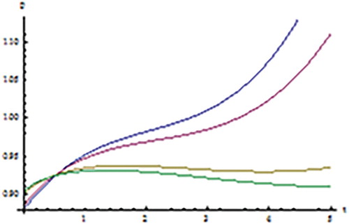
In Figure 1, we draw 3D graphic for the FGE with AB fractional operator and in Figure 2, we plot the approximate solution $p(\varkappa ,\tau )$ by using FHPTM for $\alpha =0.75,0.8,0.95,1.$ These figures show that the converging of the numerical solutions to the analytical solution connected to the exact error and the order of the solution becomes smaller as the order of the solution is increasing.

Figure 1. The 3D graphic for the FGE with AB fractional operator when $\alpha =\mathrm{0.85.}$ $ϵ=1$.

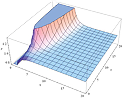
Figure 2. The 2D graphic of the FGE for different value of α when $\varkappa =2.$ $ϵ=1$.

6. Final remarks

In this study, the time fractional Gardner equation is analysed for Atangana–Baleanu fractional operator with Mittag-Leffler kernel. We applied the fractional homotopy perturbation transform method for the time fractional Gardner equation with Caputo–Fabrizio, Liouville–Caputo and Atangana–Baleanu fractional-order derivatives. We obtained approximate solutions of the equation with these different fractional-order derivatives. We showed the existence and uniqueness of the solutions for FGE. We compared these approximate solutions with each other via graphical and numerical consequences. From these conclusions, we can say that the FGE with fractional AB derivative is suitable for examining many problems in the fields of science and engineering.

Disclosure statement

No potential conflict of interest was reported by the authors.

ORCID

Zeliha Korpinar http://orcid.org/0000-0001-6658-131X

Mustafa Inc http://orcid.org/0000-0003-4996-8373

Mustafa Bayram http://orcid.org/0000-0002-2994-7201

References

- Kilbas AA, Srivastava HM, Trujillo JJ. Theory and applications of fractional differential equations. Amsterdam: Elsevier; 2006.
- Podlubny I. Fractional differential equation. San Diego, CA: Academic Press; 1999.
- Owolabi KM. Numerical analysis and pattern formation process for space-fractional superdiffusive systems. Discrete Contin Dyn Sys-S. 2019;12(3):543–566. doi: 10.3934/dcdss.2019036
- Samko SG, Kilbas AA, Marichev OI. Fractional integrals and derivatives: theory and applications. Philadelphia, Switzerland: Gordon and Breach; 1993.
- Inc M, Korpinar ZS, Al Qurashi MM, et al. A new method for approximate solution of some nonlinear equations: residual power series method. Adv Mech Engin. 2016;8(4):1–7. doi: 10.1177/1687814016644580
- Tchier F, Inc M, Korpinar ZS, et al. Solution of the time fractional reaction-diffusion equations with residual power series method. Adv Mech Engin. 2016;8(10):1–10. doi: 10.1177/1687814016670867
- Korpinar Z. On numerical solutions for the Caputo-Fabrizio fractional heat-like equation. Thermal Sci. 2018;22(1):87–95. doi: 10.2298/TSCI170614274K
- Abdeljawad T, Baleanu D. Discrete fractional differences with nonsingular discrete Mittag-Leffler kernels. Adv Differ Equ. 2016;2016:232. doi: 10.1186/s13662-016-0949-5
- Owolabi KM, Atangana A. Analysis of mathematics and numerical pattern formation in superdiffusive fractional multicomponent system. Adv Appl Math Mech. 2017;9:1438–1460. doi: 10.4208/aamm.OA-2016-0115
- Abdeljawad T, Baleanu D. Integration by parts and its applications of a new nonlocal fractional derivative with Mittag-Leffler nonsingular kernel. J Nonlinear Sci Appl. 2017;10(3):1098–1107.
- Abdeljawad T. A Lyapunov type inequality for fractional operators with nonsingular Mittag-Leffler kernel. J Inequal Appl. 2017;2017:130. doi: 10.1186/s13660-017-1400-5
- Abdeljawad T, Al-Mdallal QM. Discrete Mittag-Leffler kernel type fractional difference initial value problems and Gronwalls inequality. J Computat Appl Math. 2018;339:218–230. doi: 10.1016/j.cam.2017.10.021
- Abdeljawad T, Madjidi F. Lyapunov type inequalities for fractional difference operators with discrete Mittag-Leffler kernels of order 2<α<5/2. European Phys J Special Topic. 2017;226:3355–3368. doi: 10.1140/epjst/e2018-00004-2
- Zhang Y, Baleanu D, Yang X-J. New solutions of the transport equations in porous media within local fractional derivative. Proc Roman Academy. 2016;17:230–236.
- Khan H, Gómez-Aguilar JF, Khan A, et al. Stability analysis for fractional order advection-reaction diffusion system. Phys A. 2019;521:737–751. doi: 10.1016/j.physa.2019.01.102
- Khan H, Chen W, Sun H. Analysis of positive solution and Hyers-Ulam stability for a class of singular fractional differential equations with p-Laplacian in Banach space. Math Method Appl Sci. 2018;41(9):9321–9334.
- Gómez-Aguilar JF, López-López MG, Alvarado-Martínez VM, et al. Chaos in a cancer model via fractional derivatives with exponential decay and Mittag-Leffler law. Entropy. 2017;19:681. doi: 10.3390/e19120681
- Khan H, Khan A, Chen W, et al. Stability analysis and a numerical scheme for fractional Klein-Gordon equations. Math Meth Appl Sci. 2018;42(2):723–732. doi: 10.1002/mma.5375
- Khan Y, Wu Q. Homotopy perturbation transform method for nonlinear equations using he's polynomials. Comput Math Appl. 2011;61(8):1963–1967. doi: 10.1016/j.camwa.2010.08.022
- Goswami A, Singh J, Kumar D. A reliable algorithm for KdV equations arising in warm plasma. Nonlinear Eng. 2016;5(1):7–16. doi: 10.1515/nleng-2015-0024
- Kumar D, Singh J, Baleanu D. A new fractional model for convective straight fins with temperature-dependent thermal conductivity. Therm Sci. 2017;1:1–12.
- Kumar D, Singh J, Baleanu D, et al. Analysis of regularized long-wave equation associated with a new fractional operator with Mittag-Leffler type kernel. Physica A. 2018;492:155–167. doi: 10.1016/j.physa.2017.10.002
- Inc M. Investigation of the logarithmic-KdV equation involving Mittag-Leffler type kernel with Atangana–Baleanu derivative. Physica A. 2018;506:520–531. doi: 10.1016/j.physa.2018.04.092
- Ali M, Alquran M, Mohammad M. Solitonic solutions for homogeneous KdV systems by homotopy analysis method. J Appl Math. 2012;2012:10. Article ID 569098. doi: 10.1155/2012/569098
- Pandir Y, Duzgun HH. New exact solutions of time fractional gardner equation by using new version of F-expansion method. Commun Theor Phys. 2017;67:9–14. doi: 10.1088/0253-6102/67/1/9
- Iyiola OS, Olayinka OG. Analytical solutions of time-fractional models for homogeneous Gardner equation. Ain Shams Engin J. 2014;5:999–1004. doi: 10.1016/j.asej.2014.03.014
- Atangana A, Baleanu D. New fractional derivative with nonlocal and non-singular kernel, theory and application to heat transfer model. Therm Sci. 2016;20(2):763–769. doi: 10.2298/TSCI160111018A
- Abdeljawad T. Different type kernel h-fractional differences and their fractional hsums. Chaos Solitons Fractals. 2018;116:146156. doi: 10.1016/j.chaos.2018.09.022
- Saad KM, Atangana A, Baleanu D. New fractional derivatives with non-singular kernel applied to the Burgers equation. Chaos. 2018;28:063109. doi: 10.1063/1.5026284
- Yadav S, Pandey RK, Shukla AK. Numerical approximations of Atangana-Baleanu Caputo derivative and its application. Chaos Solitons Fractals. 2019;118:58–64. doi: 10.1016/j.chaos.2018.11.009
- Chatibi Y, El Kinani EH, Ouhadan A. Variational calculus involving nonlocal fractional derivative with Mittag-Lefler kernel. Chaos Solitons Fractals. 2019;118:117–121. doi: 10.1016/j.chaos.2018.11.017
- Koca I. Efficient numerical approach for solving fractional partial differential equations with non-singular kernel derivatives. Chaos Solitons Fractals. 2018;116:278–286. doi: 10.1016/j.chaos.2018.09.038
- Abdeljawad T, Baleanu D. On fractional derivatives with generalized Mittag-Leffler kernels. Adv Differ Equ. 2018;2018:468. doi: 10.1186/s13662-018-1914-2
- Jarad F, Abdeljawad T, Hammouch Z. On a class of ordinary differential equations in the frame of Atangana-Baleanu fractional derivative. Chaos Solitons Fractals. 2018;117:16–20. doi: 10.1016/j.chaos.2018.10.006
- Abdeljawad T. Fractional operators with generalized Mittag-Leffler kernels and their differintegrals. Chaos. 2019;29:023102. doi: 10.1063/1.5085726