
 ?Mathematical formulae have been encoded as MathML and are displayed in this HTML version using MathJax in order to improve their display. Uncheck the box to turn MathJax off. This feature requires Javascript. Click on a formula to zoom.
ABSTRACT
This paper poses the Riccati–Bernoulli sub-ODE method in order to find the exact (random) travelling wave solutions for the (2+1)-dimensional cubic nonlinear Klein–Gordon (cKG) equation and the (2+1)-dimensional nonlinear Zakharov–Kuznetsov modified equal width (ZK-MEW) equation. The obtained travelling wave solutions are expressed by the hyperbolic, trigonometric and rational functions. Indeed, these solutions reflect some interesting physical interpretation for nonlinear phenomena. We discuss our method in deterministic case and in a random case. Additionally, we can show and discuss this method under some random distributions. Finally, some three-dimensional graphics of some solutions have been illustrated.
1. Introduction
Nonlinear phenomena arise in many areas of applied science, such as fluid mechanics, biology, optical fibres, plasma physics and so on. Actually, these phenomena can be described by nonlinear partial differential equations (NPDEs), see [Citation1–13]. Due to the importance of these NPDEs, searching for exact solutions for these equations has become more and more attractive field in different branches of physics and applied mathematics. Therefore investigating new methods to solve more complicated problems. Thus, many new methods have been proposed, such as the tanh-sech method [Citation14–16], Jacobi elliptic function method [Citation17–19], exp-function method [Citation20,Citation21], sine-cosine method [Citation22–24], homogeneous balance method [Citation25,Citation26], F-expansion method [Citation27,Citation28], extended tanh-method [Citation29,Citation30], expansion method [Citation31,Citation32]. Indeed, there are recent development in analytical and numerical methods for finding solutions for NPDEs, see [Citation33–44] and references therein.
In this paper, we use the Riccati–Bernoulli sub-ODE method [Citation11,Citation12,Citation45–47], to construct exact solutions, solitary wave solutions for the (2+1)-dimensional cubic nonlinear Klein–Gordon (cKG) equation and the (2+1)-dimensional nonlinear Zakharov–Kuznetsov modified equal width (ZK-MEW) equation. If we get a solution of NPDEs, we obtain new infinite sequence of solutions of these equations by using a Bäcklund transformation. Actually, we give new solutions and show that this method is efficient, powerful and vital for solving other type of NPDEs. Moreover the Riccati–Bernoulli sub-ODE method has an interesting feature, namely it is give infinite solutions. Indeed all presented solutions have so important contribution for the explanation of some practical physical phenomena and further nonlinear problems. To the best of our knowledge, no previous research work has been done using Riccati–Bernoulli sub-ODE method for solving the cKG equation and the ZK-MEW equation.
In many recent models, studying has ensued about the role of random or noise variables that end up as basic variables in predictive models. Therefore, one might think that the randomness part or the randomness effectiveness might be a normal outcome in many models. There are several difficulties in the study of stochastic models which may be as stochastic differential equations (SDEs) [Citation48,Citation49], or stochastic partial differential equations (SPDEs) [Citation50,Citation51]. As result, we implemented the Riccati–Bernoulli sub-ODE method for finding the exact stochastic solutions of the (2+1)-dimensional stochastic cKG equation and the (2+1)-dimensional nonlinear stochastic ZK-MEW equation, when the parameters are assigned random variables. In order to find the conditions for our method in random case we will state the stability and convergence theorem.
The rest of the paper is given as follows. Section 2 describes the Riccati–Bernoulli sub-ODE method and a Bäcklund transformation of the Riccati–Bernoulli equation. In Sections 3, we apply the Riccati–Bernoulli sub-ODE method to solve the (2+1)-dimensional cGK equation and the (2+1)-dimensional nonlinear ZK-MEW equation. Additionally, in Section 4 we can discuss the Random Riccati–Bernoulli sub-RODE method. Finally, in Section 6 we give the conclusions.
2. The Riccati–Bernoulli sub-ODE method
Consider the following nonlinear evolution equation
(1)
(1) where P is a polynomial in
and its partial derivatives with even highest order derivatives and nonlinear terms.
Step 1. Let
(2)
(2) then Equation (Equation1
(1)
(1) ) reduces to a nonlinear ordinary differential equation ODE:
(3)
(3)
Step 2. Assume the solution of Equation (Equation3(3)
(3) ) takes the form
(4)
(4) where a,b,c and n are constants to be determined. From Equation (Equation4
(4)
(4) ), we get
(5)
(5)
(6)
(6)
2.1. Classification of the solutions
The solutions for the Riccati–Bernoulli Equation (Equation4(4)
(4) ) are:
Case 1: When n=1, then
(7)
(7) Case 2: When
, b=0 and c=0, then
(8)
(8) Case 3: When
,
and c=0, then
(9)
(9) Case 4: When
,
and
, then
(10)
(10) and
(11)
(11) Case 5: When
,
and
, then
(12)
(12) and
(13)
(13) Case 6: When
,
and
, then
(14)
(14) Here μ is an arbitrary constant.
Step 3. Substituting the derivatives of u into Equation(Equation3(3)
(3) ) gives an algebraic equation of u. We can determine n, by using the symmetry of the right-hand item of Equation (Equation4
(4)
(4) ) and setting the highest power exponents of u to equivalence in Equation (Equation3
(3)
(3) ). We compare the coefficients of
gives a set of algebraic equations for
. Solving these equations and superseding n,a,b,c,v, and
into Equations (Equation7
(7)
(7) )–(Equation14
(14)
(14) )), then the solutions of Equation (Equation1
(1)
(1) ) is obtained.
2.2. Bäcklund transformation
When and
are the solutions of Equation (Equation4
(4)
(4) ), we get
namely
(15)
(15) Integrating Equation (Equation15
(15)
(15) ) once with respect to ξ, we get a Bäcklund transformation of Equation (Equation4
(4)
(4) ) as follows:
(16)
(16) where
and
are arbitrary constants.
The Equation (Equation16(16)
(16) ) is used to get infinite sequence of solutions for Equation (Equation4
(4)
(4) ) and consequently Equation (Equation1
(1)
(1) ).
3. Applications
3.1. The (2+1)-dimensional cKG equation
Here we solve the (2+1)-dimensional cKG equation, see [Citation52], which given as follows:
(17)
(17) where α and β are non zero constants. This equation prescribes many problems in classical (quantum) mechanics, solitons and condensed matter physics. For example, it models the dislocations in crystals and the motion of rigid pendula attached to a stretched wire [Citation53]. Using the travelling wave transformation
(18)
(18) where α and β are real constants.
Equation (Equation17(17)
(17) ) transforms into the following ODEs, using (Equation18
(18)
(18) ):
(19)
(19) Substituting Equations (Equation5
(5)
(5) ) into Equation (Equation19
(19)
(19) ), we obtain
(20)
(20) Setting n=0, Equation (Equation20
(20)
(20) ) is reduced to
(21)
(21) Setting each coefficient of
to zero, we get
(22)
(22)
(23)
(23)
(24)
(24)
(25)
(25) Solving Equations (Equation22
(22)
(22) )–(Equation25
(25)
(25) ), we get
(26)
(26)
(27)
(27)
(28)
(28) Case I. When
, superseding Equations(Equation26
(26)
(26) )–(Equation28
(28)
(28) ) and (Equation18
(18)
(18) ) into Equations (Equation10
(10)
(10) ) and (Equation11
(11)
(11) ), then the solutions of Equation (Equation17
(17)
(17) ) is,
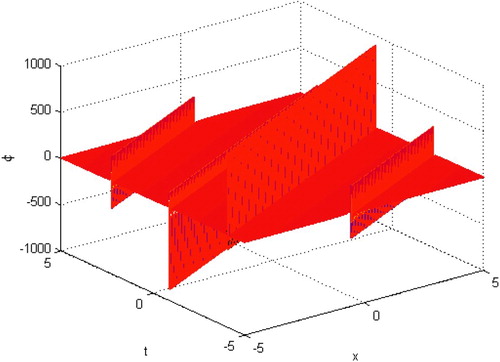
(29)
(29) and
(30)
(30) where α, β and ζ, and μ are arbitrary constants. The solution
is depicted in Figure .
Figure 1. The solution with α = 1, β = 2, λ = 2, y=n=0 and
.
Case II. When , superseding Equations (Equation26
(26)
(26) )–(Equation28
(28)
(28) ) and (Equation18
(18)
(18) ) into Equations (Equation12
(12)
(12) ) and (Equation13
(13)
(13) ), then the solutions of Equation (Equation17
(17)
(17) ) is,
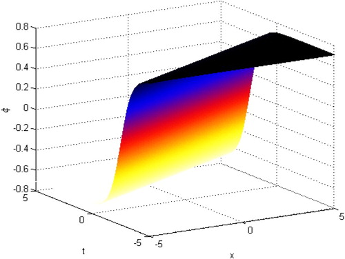
(31)
(31) and
(32)
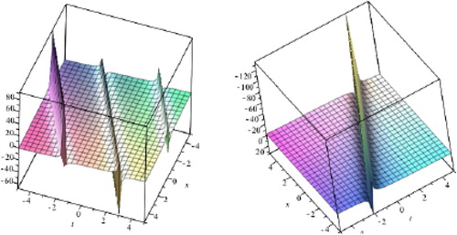
(32) where α, β and ζ and μ are arbitrary constants. The solution
is depicted in Figure .
Figure 2. The solution with α = -1, β = 2, λ = 2, y=n=0 and
.
Case III. When b=0 and c=0, the solution of Equation (Equation17(17)
(17) ) is
(33)
(33) where λ and μ are arbitrary constants.
3.1.1. Physical interpretation
Here, physical interpretations of the solutions are illustrated to show the effectiveness of the Riccati–Bernoulli sub-ODE method for seeking exact solitary wave solution and periodic travelling wave solution of Equations (Equation17(17)
(17) ). The wave speed
or
and the nonzero constants α and β play an useful role in the physical structure of the solutions obtained in Equations (Equation29
(29)
(29) )–(Equation32
(32)
(32) ) as we clarify:
If
and
If
If
If
If
If
If
If
3.2. The (2+1)-dimensional nonlinear ZK-MEW equation
Here we solve the (2+1)-dimensional nonlinear ZK-MEW equation, [Citation54]. This equation given as follows:
(34)
(34) where α, β and γ are non zero constants. Here, x is the spatial domain and t is the time.
is the evolution term,
is the nonlinear term, and
is the dispersion term. Using the travelling wave transformation
(35)
(35) where α and β are real constants.
Equation (Equation34(34)
(34) ) transforms into the following ODEs, using (Equation35
(35)
(35) ):
(36)
(36) with zero constant of integration. Substituting Equations (Equation5
(5)
(5) ) into Equation (Equation36
(36)
(36) ), we obtain
(37)
(37) Setting n=0, Equation (Equation37
(37)
(37) ) is reduced to
(38)
(38) Putting each coefficient of
to zero, we have
(39)
(39)
(40)
(40)
(41)
(41)
(42)
(42) Solving Equations (Equation39
(39)
(39) )–(Equation42
(42)
(42) ), we get
(43)
(43)
(44)
(44)
(45)
(45) Case I. When
, substituting Equations (Equation43
(43)
(43) )–(Equation45
(45)
(45) ) and (Equation35
(35)
(35) ) into Equations (Equation10
(10)
(10) ) and (Equation11
(11)
(11) ), we obtain the exact wave solutions of Equation (Equation34
(34)
(34) ),
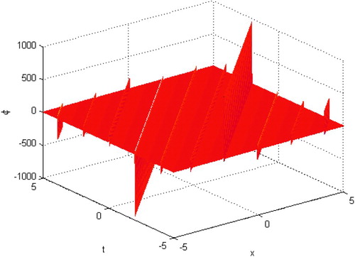
(46)
(46) and
(47)
(47) where λ, α, β, γ, ϵ, and μ are arbitrary constants. The solution
is depicted in Figure .
Figure 3. The solution with α = 2.5, λ=1, β = 0.2, γ = 0.1, ε=0.2, y=n=0 and
.
Case II. When , substituting Equations (Equation43
(43)
(43) )–(Equation45
(45)
(45) ) and (Equation35
(35)
(35) ) into Equations (Equation12
(12)
(12) ) and (Equation13
(13)
(13) ), we get exact travelling wave solutions of Equation (Equation34
(34)
(34) ),
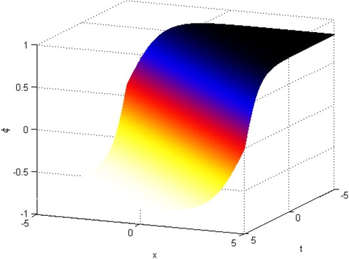
(48)
(48) and
(49)
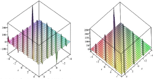
(49) where λ, α, β, γ, ε, and μ are arbitrary constants. The solution
is depicted in Figure .
Figure 4. The solution with α = -1.5, λ=1, β = 0.6, γ = 1.3, ε = 1.2, y=n=0 and
.
Case III. When b=0 and c=0, the solution of Equation (Equation34(34)
(34) ) is
(50)
(50) where ε, λ and μ are arbitrary constants.
Remark 3.1
Applying Equation (Equation16(16)
(16) ) to
and
once, we can obtain an infinite solutions of Equations (Equation17
(17)
(17) ) and (Equation34
(34)
(34) ), respictively.
4. Stochastic models
In fact, the stochastic models has many applications in our life and it can be as stochastic dynamical system so, it is important for us to discuss what is the effect when dealing with these stochastic models and how to find the control of stability or the constraints on the randomness part in order to find the solution for these models. In this section, we investigate stochastic process solution of the (2+1)-dimensional Stochastic cubic nonlinear Klein–Gordon model with two random variables input and (2+1)-dimensional nonlinear stochastic ZK-MEW model with three random variables by using the Riccati–Bernoulli sub-RODE method.
4.1. The (2+1)-dimensional cubic stochastic nonlinear Klein–Gordon model
The nonlinear stochastic Klein–Gordon equation is used to model many nonlinear phenomena. In this part of the paper, a new Riccati–Bernoulli sub-RODE method for solving the (2+1)-dimensional cubic stochastic nonlinear Klein–Gordon model is proposed as follow:
(51)
(51) where α and β are non zero random variables.
As the in deterministic case we can find the solutions as follow:
When α, β are positive bounded random variables i.e. ,
,
, we get stochastic exact travelling wave solutions as follow,
(52)
(52) and
(53)
(53) where α, β are random variables and ζ, and μ are arbitrary constants. The expected value operator of the stochastic solution
,
is depicted in Figure . The variance of the stochastic solution
,
is depicted in Figure , respectively.
Figure 5. Graph of expectation of stochastic process solutions and
on the left and right, respectively with α and β have Beta distribution
, λ = 2, y=n=0 and
for Equation (Equation51
(51)
(51) ).
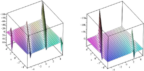
Figure 6. Graph of variance of stochastic process solutions ,
on the left and right, respectively with α and β have Beta distribution
, λ = 2, y=n=0 and
for Equation (Equation51
(51)
(51) ).
4.1.1. Theory of stability
The stochastic process solution for our problem, the (2+1)-dimensional stochastic cubic nonlinear Klein–Gordon equation is will be stable under the conditions:
α is bounded and second order random variable (
β is bounded and second order random variable (
Also, for the Riccati–Bernoulli sub-ODE method that we used must be with second order the travelling wave transformation since .
4.2. The (2+1)-dimensional stochastic nonlinear ZK-MEW equation
Stochastic nonlinear ZK-MEW equation in many areas play an important role. Therefore, solving stochastic or deterministic nonlinear ZK-MEW equation or generally, the nonlinear evolution equations has become a valuable task. For this purpose, we will try to deal with the stochastic case as follow. This equation given as follows:
(54)
(54) where α, β and γ are non zero random variables.
AS the same as in deterministic case we can find the stochastic solution relation as follow, When α, β and γ are positive bounded random variables i.e. ,
,
and
, we get stochastic exact travelling wave solutions as follow,
(55)
(55) and
(56)
(56) where α, β, γ are random variables, λ, ϵ, and μ are arbitrary constants. The expected value operator of the stochastic solution
,
is depicted in Figure . The variance of the stochastic solution
,
is depicted in Figure .
Figure 7. Graph of expectation of stochastic process solutions ,
on the left and right, respectively with α and β have Beta distribution
, λ = 1, y=n=0 and
for Equation (Equation54
(54)
(54) ).
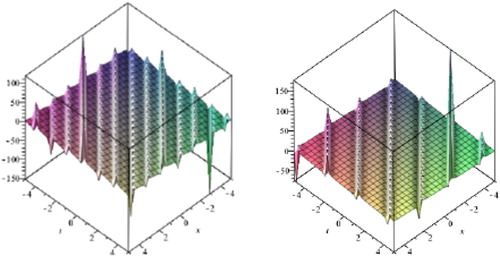
Figure 8. Graph of variance of stochastic process solutions ,
on the left and right, respectively with α and β have Beta distribution
, λ = 1, y=n=0 and
for Equation (Equation54
(54)
(54) ).
4.2.1. Theory of stability
The stochastic process solution for our problem, the (2+1)-dimensional nonlinear stochastic Zakharov–Kuznetsov modified equal width (SZK-MEW) equation is will be stable under the conditions:
α is bounded and second order random variable (
β is bounded and second order random variable (
γ is bounded and second order random variable (
Also, for the Riccati–Bernoulli sub-ODE method that we used must be with second order the travelling wave transformation since .
Remark 4.1
The Riccati–Bernoulli sub-ODE method has been successfully applied to find new travelling wave solutions for the (2+1)-dimensional cubic nonlinear Klein–Gordon equation and the (2+1)-dimensional nonlinear Zakharov–Kuznetsov modified equal width (ZK-MEW) models. As a result, we obtained many new exact solutions including rational function, hyperbolic function and trigonometric function solutions. It can be concluded that this method is a very robust and efficient technique to find the exact solutions for a large class of NPDEs. Moreover, from Remark 3.1 we find that the Riccati–Bernoulli sub-ODE method gives an infinite sequence of solutions. Moreover, we implemented the Riccati–Bernoulli sub-ODE method for finding the exact stochastic solutions of the proposed models, when the parameters are assigned random variables. We also state the stability and convergence theorem to find the conditions for the proposed method in random case.
5. Comparisons
We compare the results presented in this paper with other results in order to show that the Riccati–Bernoulli sub-ODE is powerful,efficient and adequate.
Wang et al. [Citation52] have presented only five solutions for the cKG equation, using the multi-function expansion method. Whereas Khan et al. [Citation55] given eight solutions, using the modified simple equation (MSE) method. Comparing these results with presented result in this paper, we deduce that the Riccati–Bernoulli sub-ODE method gives many new exact travelling wave solutions along with additional free parameters. Thus, the Riccati–Bernoulli sub-ODE method is more effective in providing many new solutions than these two methods.
Wazwaz [Citation54] has presented only four solutions for the ZK-MEW equation, using the sine-cosine method and has introduced four solutions, using the tanh-method. On the other hand, we give many new exact travelling wave solutions with numerous free parameters.
Thus, the Riccati–Bernoulli sub-ODE method superior to other methods.
6. Conclusions
We have introduced the (2+1)-dimensional cubic nonlinear Klein–Gordon equation and the (2+1)-dimensional nonlinear Zakharov–Kuznetsov modified equal width (ZK-MEW) models in deterministic case and also, if we have some disturbance in their coefficients. We have proposed Riccati–Bernoulli sub-ODE method in order to find the exact travelling wave solutions for these models, additionally, to find the stochastic process solution. The physical cases for the solution of the (2+1)-dimensional cKG equation is discussed. The stochastic process solutions are studied for our models by stability control on the randomness part. The statistical moments are computed.
Acknowledgments
The authors thank the editor and referees for their valuable comments and suggestions.
Disclosure statement
No potential conflict of interest was reported by the authors.
ORCID
Mahmoud A.E. Abdelrahman http://orcid.org/0000-0002-7351-2088
M. A. Sohaly http://orcid.org/0000-0001-5971-0048
Abdulghani Alharbi http://orcid.org/0000-0002-1430-4684
References
- Abdelrahman MAE, Kunik M. The interaction of waves for the ultra-relativistic Euler equations. J Math Anal Appl. 2014;409:1140–1158. doi: 10.1016/j.jmaa.2013.07.009
- Abdelrahman MAE, Kunik M. A new front tracking scheme for the ultra-relativistic Euler equations. J Comput Phys. 2014;275:213–235. doi: 10.1016/j.jcp.2014.06.051
- Abdelrahman MAE, Kunik M. The ultra-relativistic Euler equations. Math Meth Appl Sci. 2015;38:1247–1264. doi: 10.1002/mma.3141
- Abdelrahman MAE. Global solutions for the ultra-relativistic Euler equations. Nonlinear Anal. 2017;155:140–162. doi: 10.1016/j.na.2017.01.014
- Abdelrahman MAE. On the shallow water equations. Z Naturforsch. 2017;72(9a):873–879.
- Abdelrahman MAE. Numerical investigation of the wave-front tracking algorithm for the full ultra-relativistic Euler equations. Int J Nonlinear Sci Numer Simul. doi: 10.1515/ijnsns-2017-0121.
- Razborova P, Ahmed B, Biswas A. Solitons, shock waves and conservation laws of Rosenau-KdV-RLW equation with power law nonlinearity. Appl Math Inf Sci. 2014;8(2):485–491. doi: 10.12785/amis/080205
- Biswas A, Mirzazadeh M. Dark optical solitons with power law nonlinearity using G′/G-expansion. Optik. 2014;125:4603–4608. doi: 10.1016/j.ijleo.2014.05.035
- Younis M, Ali S, Mahmood SA. Solitons for compound KdV Burgers equation with variable coefficients and power law nonlinearity. Nonlinear Dyn. 2015;81:1191–1196. doi: 10.1007/s11071-015-2060-y
- Bhrawy AH. An efficient Jacobi pseudospectral approximation for nonlinear complex generalized Zakharov system. Appl Math Comput. 2014;247:30–46.
- Abdelrahman MAE, Sohaly MA. Solitary waves for the modified Korteweg-De Vries equation in deterministic case and random case. J Phys Math. 2017;8(1). doi: 10.4172/2090-0902.1000214.
- Abdelrahman MAE, Sohaly MA. Solitary waves for the nonlinear Schrödinger problem with the probability distribution function in stochastic input case. Eur Phys J Plus (2017).
- Abdelrahman MAE, Sohaly MA. The development of the deterministic nonlinear PDEs in particle physics to stochastic case. Results Phys. 2018;9:344–350. doi: 10.1016/j.rinp.2018.02.032
- Malfliet W. Solitary wave solutions of nonlinear wave equation. Am J Phys. 1992;60:650–654. doi: 10.1119/1.17120
- Malfliet W, Hereman W. The tanh method: exact solutions of nonlinear evolution and wave equations. Phys Scr. 1996;54:563–568. doi: 10.1088/0031-8949/54/6/003
- Wazwaz AM. The tanh method for travelling wave solutions of nonlinear equations. Appl Math Comput. 2004;154:714–723.
- Dai CQ, Zhang JF. Jacobian elliptic function method for nonlinear differential difference equations. Chaos Solutions Fract. 2006;27:1042–1049. doi: 10.1016/j.chaos.2005.04.071
- Fan E, Zhang J. Applications of the Jacobi elliptic function method to special-type nonlinear equations. Phys Lett A. 2002;305:383–392. doi: 10.1016/S0375-9601(02)01516-5
- Liu S, Fu Z, Liu s, et al. Jacobi elliptic function expansion method and periodic wave solutions of nonlinear wave equations. Phys Lett A. 2001;289:69–74. doi: 10.1016/S0375-9601(01)00580-1
- He JH, Wu XH. Exp-function method for nonlinear wave equations. Chaos Solitons Fractals. 2006;30:700–708. doi: 10.1016/j.chaos.2006.03.020
- Aminikhad H, Moosaei H, Hajipour M. Exact solutions for nonlinear partial differential equations via Exp-function method. Numer Methods Partial Differ Equ. 2009;26:1427–1433.
- Wazwaz AM. Exact solutions to the double sinh-Gordon equation by the tanh method and a variable separated ODE method. Comput Math Appl. 2005;50:1685–1696. doi: 10.1016/j.camwa.2005.05.010
- Wazwaz AM. A sine-cosine method for handling nonlinear wave equations. Math Comput Model. 2004;40:499–508. doi: 10.1016/j.mcm.2003.12.010
- Yan C. A simple transformation for nonlinear waves. Phys Lett A. 1996;224:77–84. doi: 10.1016/S0375-9601(96)00770-0
- Fan E, Zhang H. A note on the homogeneous balance method. Phys Lett A. 1998;246:403–406. doi: 10.1016/S0375-9601(98)00547-7
- Wang ML. Exct solutions for a compound KdV-Burgers equation. Phys Lett A. 1996;213:279–287. doi: 10.1016/0375-9601(96)00103-X
- Ren YJ, Zhang HQ. A generalized F-expansion method to find abundant families of Jacobi elliptic function solutions of the (2+1)-dimensional Nizhnik-Novikov-Veselov equation. Chaos Solitons Fract. 2006;27:959–979. doi: 10.1016/j.chaos.2005.04.063
- Zhang JL, Wang ML, Wang YM, et al. The improved F-expansion method and its applications. Phys Lett A. 2006;350:103–109. doi: 10.1016/j.physleta.2005.10.099
- Fan E. Extended tanh-function method and its applications to nonlinear equations. Phys Lett A. 2000;277:212–218. doi: 10.1016/S0375-9601(00)00725-8
- Wazwaz AM. The extended tanh method for abundant solitary wave solutions of nonlinear wave equations. Appl Math Comput. 2007;187:1131–1142.
- Wang ML, Zhang JL, Li XI. The (G′/G)- expansion method and travelling wave solutions of nonlinear evolutions equations in mathematical physics. Phys Lett A. 2008;372:417–423. doi: 10.1016/j.physleta.2007.07.051
- Zhang S, Tong JL, Wang W. A generalized (G′/G)- expansion method for the mKdv equation with variable coefficients. Phys Lett A. 2008;372:2254–2257. doi: 10.1016/j.physleta.2007.11.026
- Ferdous F, Hafez MG, Biswas A, et al. Oblique resonant optical solitons with Kerr and parabolic law nonlinearities and fractional temporal evolution by generalized exp(φ(ξ))-expansion. Optik. 2019;178:439–448. doi: 10.1016/j.ijleo.2018.10.016
- Ferdous F, Hafez MG. Nonlinear time fractional Korteweg-de Vries equations for the interaction of wave phenomena in fluid-filled elastic tubes. Eur Phys J Plus. 2018;133:384. doi: 10.1140/epjp/i2018-12195-6
- Ferdous F, Hafez MG. Oblique closed form solutions of some important fractional evolution equations via the modified Kudryashov method arising in physical problems. J Ocean Eng Sci. 2018;3:244–252. doi: 10.1016/j.joes.2018.08.005
- Hafez MG, Talukder MR, Ali MH. New analytical solutions for propagation of small but finite amplitude ion-acoustic waves in a dense plasma. Waves Random Complex Media. 2016;26(1):68–79. doi: 10.1080/17455030.2015.1111543
- Hafez MG. Exact solutions to the (3+1)-dimensional coupled Klein-Gordon-Zakharov equation using expexpansion method. Alex Eng J. 2016;55:1635–1645. doi: 10.1016/j.aej.2016.02.010
- Hafez MG. New travelling wave solutions of the (1+1)-dimensional cubic nonlinear Schrodinger equation using novel (G′/G)-expansion method. Beni-Suef Univ J Basic Appl Sci. 2016;5(2):109–118. doi: 10.1016/j.bjbas.2016.03.003
- Hafez MG, Sakthivel R, Talukder MR. Some new electrostatic potential functions used to analyze the ion-acoustic waves in a Thomas Fermi plasma with degenerate electrons. Chin J Phys. 2015;53(7):120901-1–120901-13.
- Hafez MG, Alam MN, Akbar MA. Traveling wave solutions for some important coupled nonlinear physical models via the coupled Higgs equation and the Maccari system. J King Saud Univ. 2015;27:105–112. doi: 10.1016/j.jksus.2014.09.001
- Yaslan HC, Girgin E. New exact solutions for the conformable space-time fractional KdV, CDG, (2+1)-dimensional CBS and (2+1)-dimensional AKNS equations. J Taibah Univ Sci. 2018;12:309–314. doi: 10.1080/16583655.2018.1469283
- Alam MN, Alam MM. An analytical method for solving exact solutions of a nonlinear evolution equation describing the dynamics of ionic currents along microtubules. J Taibah Univ Sci. 2017;11:939–948. doi: 10.1016/j.jtusci.2016.11.004
- Nuruddeen RI, Nass AM. Exact solitary wave solution for the fractional and classical GEW-burgers equations: an application of kudryashov method. J Taibah Univ Sci. 2018;12:309–314. doi: 10.1080/16583655.2018.1469283
- Ebrahimi Ghogdia S, Ghomanjani F, Saberi-Nadjafi J. Expansion of the Exp-function method for solving systems of two-dimensional NavierStokes equations. J Taibah Univ Sci. 2015;9:121–125. doi: 10.1016/j.jtusci.2014.07.009
- Abdelrahman MAE. A note on Riccati-Bernoulli sub-ODE method combined with complex transform method applied to fractional differential equations. Nonlinear Eng Model Appl. (2018). doi: 10.1515/nleng-2017-0145.
- Hassan SZ, Abdelrahman MAE. Solitary wave solutions for some nonlinear time-fractional partial differential equations. Pramana – J Phys. 2018;91:67. doi:10.1007/s12043-018-1636-8.
- Yang XF, Deng ZC, Wei Y. A Riccati-Bernoulli sub-ODE method for nonlinear partial differential equations and its application. Adv Differ Equ. 2015;1:117–133. doi: 10.1186/s13662-015-0452-4
- El-Tawil MA, Sohaly MA. Mean square numerical methods for initial value random differential equations. Open J Discrete Math. 2011;1.02:66. doi: 10.4236/ojdm.2011.12009
- El-Tawil MA, Sohaly MA. Mean square convergent finite difference scheme for random first order partial differential equations. The Egyptian Mathematical Society, International Conference on Mathematics. Trends and Development ICMTD12.
- Navarro-Quiles A, Romero JV, Rosell MD, Sohaly MA. Approximating the solution stochastic process of the random Cauchy one-dimensional heat model. Abs Appl Anal. 2016;2016. Article ID 5391368, 7 pages, 2016. doi:10.1155/2016/5391368.
- Sohaly MA. Mean square convergent three and five points finite difference scheme for stochastic parabolic partial differential equations. EJMAA. 2014;2(1):164–171.
- Wang Z, Zhang HQ. Many new kinds exact solutions to (2+1)-dimensional Burgers equation and Klein-Gordon equation used a new method with symbolic computation. Appl Math Comput. 2007;186:693–704.
- Yusufoglu E. The variational iteration method for studying the Klein-Gordon equation. Appl Math Lett. 2008;21:669–674. doi: 10.1016/j.aml.2007.07.023
- Wazwaz AM. Exact solutions for the ZK-MEW equation by using the tanh and sine-cosine methods. Int J Comput Math. 2005;82(6):699–708. doi: 10.1080/00207160512331329069
- Khan K, Akbar MA. Exact Solutions of the (2+1)-dimensional cubic Klein-Gordon Equation and the (3+1)-dimensional Zakharov-Kuznetsov equation using the modified simple equation method. J Assoc Arab Univ Basic Appl Sci. 2014;15:74–81.