The generalized odd Burr III family of distributions: properties, applications and characterizations

ABSTRACT

A new class of continuous distributions with two extra shape parameters is introduced named the generalized odd Burr III (GOBIII) family of distributions. The expression of density can be written as a linear combination of exponentiated densities related to baseline model. The basic properties such as ordinary moments, quantile and generating functions, two entropy measures and order statistics are derived. Three special models of proposed family are presented. Characterizations related to truncated moments and hazard function for GOBIII-G distribution are derived. Method of maximum likelihood is used to estimate the model parameters. We study the behaviour of the estimators by means of simulations. The importance of the new family is illustrated using two real data sets. The real data applications suggest that this family can provide better fits than other competitive distributions. The significance of GOBIII-G family lies in its capability to fit symmetric as well as skewed type of data.

KEYWORDS:

• G-family
• odd Burr III
• maximum likelihood
• moment
• order statistic
• Rényi entropy

1. Introduction

Burr III distribution attracts extraordinary consideration since it includes several families of distributions and it incorporates the qualities of different distributions such as exponential and logistic distributions. The Burr III distribution extensively used in various fields such as survival and reliability analysis, environmental studies, economics, meteorology and water resources, forestry among others. This distribution is also applied to wages, income and wealth datasets. A comprehensive and suitable model is always preferred throughout the literature. So many attempts are made to enhance the flexibility of the distribution by inducting one or more parameters to the parent distribution. Numerous generators are available in the literature to derive the extended forms of distribution are a mixture of two distributions. Eugene et al. [1] derived and studied the Beta-G family of distributions and using this idea many extended forms of beta distribution proposed, for example, beta normal, beta Weibull, etc. Furthermore, researchers proposed generalized families; Kumaraswamy-G [2], Marshall–Olkin-G [3], McDonald-G [4], Weibull-G [5], Lomax-G [6], Type II half logistic-G [7], exponentiated extended-G [8], odd Fréchet-G [9], moment exponential-G [10] family of distributions. A review on well-known G-classes is reported by [11].

The cumulative distribution function (cdf) and probability density function (pdf) of Burr III distribution are respectively, given by (1) $H\left(x;c,k\right)=(1+x^{-c}{)}^{-k}$(1) (2) $h\left(x;,c,k\right)=ck{x}^{-c-1}(1+x^{-c}{)}^{-k-1},x>0,c,k>0.$(2) where c and k are two shape parameters.

Recently [12] introduced the idea of T-X family of distributions and its cdf is defined as $F\left(x\right)={\int }_0^{W\left[G\left(x\right)\right]}r\left(t\right)dt,x\in R$and the cdf of Generalized Odd-G distribution is $F\left(x\right)={\int }_0^{\left[\frac{G{\left(x,\delta \right)}^{\alpha }}{1-G{\left(x,\delta \right)}^{\alpha }}\right]}r\left(t\right)dt,x\in R$Using this generator, we propose generalized odd Burr III-G (GOBIII-G) family of distributions. The suggested class is much wider and flexible.

The new family can get by integrating the Bur III density function (3) $\begin{array}{rl}F\left(x;c,k,\alpha ,\zeta \right)& =ck{\int }_0^{\frac{G{\left(x;\zeta \right)}^{\alpha }}{1-G{\left(x;\zeta \right)}^{\alpha }}}{t}^{-c-1}(1+t^{-c}{)}^{-k-1}dt\\ & ={\left\{1+{\left(\frac{1-G{\left(x;\zeta \right)}^{\alpha }}{G{\left(x;\zeta \right)}^{\alpha }}\right)}^c\right\}}^{-k}\end{array}$(3) The cdf of GOBIII-G family is obtained by (3) using baseline G. Equation (3) gives a vast family of continuous distributions and one of its special case is Odd Burr III [13].

The pdf of the GOBIII-G corresponding to Equation (3) is given by (4) $\begin{array}{rl}f\left(x;c,k,\alpha ,\zeta \right)& =ck\alpha g\left(x;\zeta \right)\frac{{\left[1-G{\left(x;\zeta \right)}^{\alpha }\right]}^{c-1}}{{\left[G\left(x;\zeta \right)\right]}^{c\alpha +1}}\\ & \times {\left\{1+{\left(\frac{1-G{\left(x;\zeta \right)}^{\alpha }}{G{\left(x;\zeta \right)}^{\alpha }}\right)}^c\right\}}^{-k-1}\end{array}$(4) where g(x; ξ) is pdf of baseline model. After this, a random variable X with density function (4) is represented by X ∼ GOBIII-G(c, k, α, $\zeta$). Or we can write simply $G\left(x\right)=G(x;\zeta )$. The density function (4) permits more flexibility and can be widely applied in numerous areas of real life. It will be manageable when baseline G(x) and g(x) are in closed-form.

The survival S(x), hazard function h(x) and reversed hazard rate τ(x) functions of X becomes (5) $S\left(x\right)=\overline{F}\left(x;c,k,\alpha ,\zeta \right)=1-{\left\{1+{\left(\frac{1-G{\left(x;\zeta \right)}^{\alpha }}{G{\left(x;\zeta \right)}^{\alpha }}\right)}^c\right\}}^{-k},$(5) (6) $\begin{array}{rl}& h\left(x;c,k,\alpha ,\zeta \right)\\ & =\frac{ck\alpha g\left(x;\zeta \right)\frac{{\left[1-G{\left(x;\zeta \right)}^{\alpha }\right]}^{c-1}}{{\left[G\left(x;\zeta \right)\right]}^{c\alpha +1}}{\left\{1+{\left(\frac{1-G{\left(x;\zeta \right)}^{\alpha }}{G{\left(x;\zeta \right)}^{\alpha }}\right)}^c\right\}}^{-k-1}}{1-{\left\{1+{\left(\frac{1-G{\left(x;\zeta \right)}^{\alpha }}{G{\left(x;\zeta \right)}^{\alpha }}\right)}^c\right\}}^{-k}},\end{array}$(6) and (7) $\tau \left(x;c,k,\alpha ,\zeta \right)=\frac{ck\alpha g\left(x;\zeta \right)\frac{{\left[1-G{\left(x;\zeta \right)}^{\alpha }\right]}^{c-1}}{{\left[G\left(x;\zeta \right)\right]}^{c\alpha +1}}}{1+{\left(\frac{1-G{\left(x;\zeta \right)}^{\alpha }}{G{\left(x;\zeta \right)}^{\alpha }}\right)}^c}.$(7)

The basic inspirations of using GOBIII-G family of distribution are:

• To extend baseline distribution, T-X family of distributions is a good generator.

• To enhance the characteristics of the baseline distribution.

• To make the shape of the proposed distribution more flexible as compared to the baseline model.

• To give special models with different trends of hazard rate function.

• To state special models having closed form of cdf and hrf.

• To provide consistently better fits than other generated distributions having the same or higher number of parameters.

2. Special models

Here, we give some special models of the GOBIII-G family of distributions, namely: the generalized odd Burr-Weibull (GOBIII-W), generalized odd Burr-Lomax (GOBIII-Lx), generalized odd Burr-Logistic (GOBIII-Log) distributions.

2.1. Generalized odd Burr III Weibull distribution

Let the Weibull distribution is the baseline distribution with probability density and cumulative distribution functions given, respectively by $\begin{array}{rl}g(x,\text{β},\gamma )& =\left(\frac{\gamma }{\text{β}}\right){\left(\frac{x}{\text{β}}\right)}^{\gamma -1}{\text{e}}^{-{\left(x/\text{β}\right)}^{\gamma }}\text{, x}\ge 0,\text{β}\text{,}\gamma >0,\\ & \mathrm{a}\mathrm{n}\mathrm{d}G(x,\text{β},\gamma )=1-{\text{e}}^{-{\left(x/\text{β}\right)}^{\gamma }}\text{.}\end{array}$Then the GOBIII–W distribution has the following cdf and pdf (8) $F\left(x\right)={\left\{1+{\left(\frac{1-{\left(\text{1 - }{\text{e}}^{-{\left(x/\text{β}\right)}^{\gamma }}\right)}^{\alpha }}{{\left(\text{1 - }{\text{e}}^{-{\left(x/\text{β}\right)}^{\gamma }}\right)}^{\alpha }}\right)}^c\right\}}^{-k},$(8) and

(9) $\begin{array}{rl}f\left(x\right)& =ck\alpha \left(\frac{\gamma }{\text{β}}\right){\left(\frac{x}{\text{β}}\right)}^{\gamma -1}\\ & \times {\text{e}}^{-{\left(x/\text{β}\right)}^{\gamma }}\frac{{\left[1-{\left(1-{\text{e}}^{-{\left(x/\text{β}\right)}^{\gamma }}\right)}^{\alpha }\right]}^{c-1}}{{\left(1-{\text{e}}^{-{\left(x/\text{β}\right)}^{\gamma }}\right)}^{c\alpha +1}}\\ & \times \left\{1+{\left(\frac{1-{\left(1-{\text{e}}^{-{\left(x/\text{β}\right)}^{\gamma }}\right)}^{\alpha }}{{(1-{\text{e}}^{-{\left(x/\text{β}\right)}^{\gamma }})}^{\alpha }}\right)}^c\right\}.\end{array}$(9)

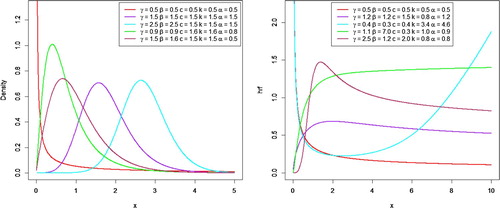
The graphs of pdf and hazard function of Generalized Odd Burr III-Weibull distribution are given in Figure 1 for specific values of parameters. The pdf of GOBIII-W is decreasing when γ < 1. The pdf curves are right-skewed when γ > 1.

Figure 1. Plots of (left) densities and (right) hazard rates of GOBIII-W distribution.

2.2. Generalized odd Burr III Lomax distribution

Let us consider the Lomax distribution with probability density and distribution functions given, respectively by $g(x,\text{β},\gamma )=\left(\gamma /\text{β}\right){\left[1+\frac{x}{\text{β}}\right]}^{-\gamma -1}\text{, }\text{β}\text{,}\gamma >0,$ and $G(x,\text{β},\gamma )=1-{\left[1+\frac{x}{\text{β}}\right]}^{-\gamma }\text{.}$

Then the GOBIII–Lx distribution has the following cdf and pdf

(10) $F\left(x\right)={\left\{1+{\left(\frac{1-{\left\{1-{\left(1+\frac{x}{\text{β}}\right)}^{-\gamma }\right\}}^{\alpha }}{{\left\{1-{\left(1+\frac{x}{\text{β}}\right)}^{-\gamma }\right\}}^{\alpha }}\right)}^c\right\}}^{-k},$(10)

and

(11) $\begin{array}{rl}f\left(x\right)& =ck\alpha \left(\gamma /\text{β}\right){\left[1+\frac{x}{\text{β}}\right]}^{-\gamma -1}\\ & \times \frac{{\left[1-{\left\{1-{\left(1+\frac{x}{\text{β}}\right)}^{-\gamma }\right\}}^{\alpha }\right]}^{c-1}}{{\left(1-{\left(1+\frac{x}{\text{β}}\right)}^{-\gamma }\right)}^{c\alpha +1}}\\ & \times {\left\{1+{\left(\frac{1-{\left\{1-{\left(1+\frac{x}{\text{β}}\right)}^{-\gamma }\right\}}^{\alpha }}{{\left\{1-{\left(1+\frac{x}{\text{β}}\right)}^{-\gamma }\right\}}^{\alpha }}\right)}^c\right\}}^{-k-1}.\end{array}$(11)

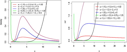
Following are the plots of density and hazard function of Generalized Odd Burr III-Lomax distribution are given below for specific values of parameters taking β = 5 (Figure 2).

Figure 2. Plots of (left) densities and (right) hazard rates of GOBIII-Lx distribution for β = 5.

2.3. Generalized odd Burr III logistic distribution

Let us consider the logistic distribution with probability density and distribution functions given, respectively by $g(x,\delta )=\delta e^{-\delta x}{(1+e^{-\delta x}{)}^{-2}}^{}\text{, }\delta >0,$ and $G(x,\delta )=(1+e^{-\delta x}{)}^{-1}\text{.}$

Then GOBIII – Log distribution has the following cdf and pdf (12) $F\left(x\right)={\left\{1+{\left(\frac{1-{\left(1+e^{-\delta x}\right)}^{-\alpha }}{{\left(1+e^{-\delta x}\right)}^{-\alpha }}\right)}^c\right\}}^{-k},$(12) and (13) $\begin{array}{rl}f\left(x\right)& =ck\alpha \delta e^{-\delta x}(1+e^{-\delta x}{)}^{-2}\frac{{\left[1-{\left(1+e^{-\delta x}\right)}^{-\alpha }\right]}^{c-1}}{{\left(1+e^{-\delta x}\right)}^{-(\alpha c+1)}}\\ & \times {\left\{1+{\left(\frac{1-{\left(1+e^{-\delta x}\right)}^{-\alpha }}{{\left(1+e^{-\delta x}\right)}^{-\alpha }}\right)}^c\right\}}^{-k-1}.\end{array}$(13)

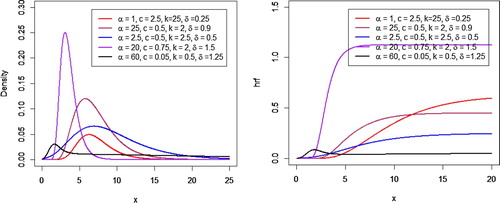
Following are the plots of density and hazard rate function of Generalized Odd Burr III-Logistic distribution for specific values of parameters (Figure 3).

Figure 3. Plots of (left) densities and (right) hazard rates of GOBIII-Log distribution.

3. Properties

In this section, we derive the expressions of some structural characteristics including ordinary, probability weighted. Further, we also derived the moment generating function, quantile function, expressions of mean deviation, order statistics, and Renyi entropy.

3.1. Quantile function

Let X denotes a random variable has the pdf (4), the quantile function; say $Q\left(u\right)$ of X is given by (14) $Q\left(u\right)=G^{-1}{\left[1+{\left(u^{\frac{-1}{k}}-1\right)}^{\frac{1}{c}}\right]}^{\frac{-1}{\alpha }},$(14) where $u$ is a uniform distribution on the interval $\left(0,1\right)$ and $G^{-1}(.)$ is the inverse function of $G(.)$.

3.2. Useful expansion

In this subsection, using binomial series expansion, the density function for GOBIII-G family is obtained. (15) $(1+z{)}^{-\text{β}}=\sum _{i=0}^{\mathrm{\infty }}(-1{)}^i\left(\begin{array}{c}\text{β}+i-1\\ i\end{array}\right)z^i,$(15) for $|z|<1,$ and β is a positive real non-integer.

Applying the binomial theorem (15) in (4), it becomes $\begin{array}{rl}f\left(x\right)& =\sum _{i=0}^{\mathrm{\infty }}ck\alpha {\left(-1\right)}^i\left(\begin{array}{c}k+i\\ i\end{array}\right)g(x,\zeta )\\ & \times \frac{{\left[1-{\left(G(x,\zeta )\right)}^{\alpha }\right]}^{c\left(i+1\right)-1}}{{\left[{\left(G(x,\zeta )\right)}^{\alpha }\right]}^{c\left(i+1\right)+\frac{1}{\alpha }}}.\end{array}$By adding and subtracting 1 we can rewrite the previous equation as follows (16) $\begin{array}{rl}f\left(x\right)& =\sum _{i=0}^{\mathrm{\infty }}ck\alpha {\left(-1\right)}^i\left(\begin{array}{c}k+i\\ i\end{array}\right)g(x,\zeta )\\ & \times \frac{{\left[1-{\left(G(x,\zeta )\right)}^{\alpha }\right]}^{c\left(i+1\right)-1}}{{\left[1-\left[1-{\left(G(x,\zeta )\right)}^{\alpha }\right]\right]}^{c\left(i+1\right)+\frac{1}{\alpha }}}.\end{array}$(16) By using the generalized binomial series (17) $(1-z{)}^{-\text{β}}=\sum _{j=0}^{\mathrm{\infty }}\left(\begin{array}{c}\text{β}+j-1\\ j\end{array}\right)z^j,$(17) where |β|>0 is a real number.

By inserting (10) in (9) the pdf become 18 $\begin{array}{rl}f\left(x\right)& =\sum _{i,j=0}^{\mathrm{\infty }}ck\alpha {\left(-1\right)}^i\left(\begin{array}{c}k+i\\ i\end{array}\right)\left(\begin{array}{c}c\left(i+1\right)+j+\frac{1}{\alpha }-1\\ j\end{array}\right)\\ & \times g(x,\zeta )[1-{\left(G(x,\zeta )\right)}^{\alpha }{]}^{c\left(i+1\right)+j-1}.\end{array}$18 18) Again using the binomial expansion (19) $(1-z{)}^{\text{β}}=\sum _{m=0}^{\mathrm{\infty }}(-1{)}^m\left(\begin{array}{c}\text{β}\\ m\end{array}\right)z^m.$(19) By inserting (19) in (18) the pdf can be written as follows (20) $f\left(x\right)=\sum _{m=0}^{\mathrm{\infty }}{\eta }_{m}g(x,\zeta )G(x,\zeta {)}^{\alpha m},$(20) where $\begin{array}{rl}{\eta }_m& =\sum _{i,j=0}^{\mathrm{\infty }}ck\alpha {\left(-1\right)}^{i+m}\left(\begin{array}{c}k+i\\ i\end{array}\right)\left(\begin{array}{c}c\left(i+1\right)+j+\frac{1}{\alpha }-1\\ j\end{array}\right)\\ & \times \left(\begin{array}{c}c\left(i+1\right)+j-1\\ m\end{array}\right),\end{array}$Another formula can be extracted from pdf (20), which gives the following infinite linear combination $f\left(x\right)=\sum _{m=0}^{\mathrm{\infty }}{W}_m{h}_{\alpha m+1}\left(x\right),$where $W_i=\frac{{\eta }_m}{\alpha m+1},$ and $h_a\left(x\right)=ag(x,\zeta )G(x,\zeta {)}^{a-1},$ is the exponentiated-generated (Exp-G) density with the power parameter $a.$

Further, an expansion for the $\left[F\right(x){]}^h$ is derived, for “h” is an integer, again, using the binomial expansion (15), (17) and (19) then $\left[F\right(x){]}^h$ becomes (21) $\left[F\right(x){]}^h=\sum _{z=0}^{\mathrm{\infty }}{s}_{z}G{(x,\zeta )}^{\alpha z},$(21) where $s_z=\sum _{i,j=0}^{\mathrm{\infty }}{\left(-1\right)}^{i+z}\left(\begin{array}{c}kh+i-1\\ i\end{array}\right)\left(\begin{array}{c}ci+j-1\\ j\end{array}\right)\left(\begin{array}{c}ci+j\\ z\end{array}\right).$

3.3. Characterizations

This section is related to the characterization of GOBIII-G family of distributions in two ways: related to truncated moments and related to hazard function. Characterization is theoretically important as it is the unique way of identifying the distribution. Characterizing a distribution is an important problem which helps the researcher to see if the proposed model is the correct one.

3.3.1. Characterization based on two truncated moments

For characterization of GOBIII-G family we use the proposition based on the ratio of two truncated moments [14] and also presented in the Appendix.

Theorem 3.1:

Let X: $\mathrm{\Omega }\to \left(0,\mathrm{\infty }\right)$ be distributed as Equation (4) and (22) $q_1\left(x\right)=[G\left(x;\zeta \right){]}^{c\alpha +\alpha }{\left\{1+{\left(\frac{1-G{\left(x;\zeta \right)}^{\alpha }}{G{\left(x;\zeta \right)}^{\alpha }}\right)}^c\right\}}^{k+1}$(22) (23) $q_2\left(x\right)=q_1\left(x\right)(1-G{\left(x;\zeta \right)}^{\alpha }{)}^c\text{for}x>0.$(23) The random variable X follows GOBIII-G distribution if and only if the function η is of the form (24) $\eta \left(x\right)=\frac{1}{2}(1-G{\left(x;\zeta \right)}^{\alpha }{)}^c$(24)

Proof:

It can be seen that $\left(1-F\left(x\right)\right)E\left[q_1\left(X\right)\text{|}X\ge x\right]=k(1-G{\left[x;\xi \right]}^{\alpha }{)}^c,x>0$ $\left(1-F\left(x\right)\right)E\left[q_2\left(X\right)\text{|}X\ge x\right]=\frac{k{\left(1-G{\left[x;\xi \right]}^{\alpha }\right)}^{2c}}{2},x>0$and so $\eta \left(x\right)=\frac{1}{2}(1-G{\left(x;\zeta \right)}^{\alpha }{)}^c$As $\eta \left(x\right)q_1\left(x\right)-q_2\left(x\right)\ne 0\text{for}\text{all}x.$the proof follows.

Conversely, given $q_1\left(x\right),q_2\left(x\right)$ and $\eta \left(x\right)$ we show that the random variable X has GOBIII-G family

Here, $s^{\mathrm{\prime }}\left(x\right)=\frac{{\eta }^{\mathrm{\prime }}\left(x\right)q_1\left(x\right)}{\eta \left(x\right)q_1\left(x\right)-q_2\left(x\right)}=\frac{{\eta }^{\mathrm{\prime }}\left(x\right)}{\eta \left(x\right)-{(1-G(x;\zeta {)}^{\alpha })}^c}$ $s^{\mathrm{\prime }}\left(x\right)=\frac{c\alpha G{\left(x;\xi \right)}^{\alpha -1}g\left(x;\xi \right)}{1-G{\left(x;\xi \right)}^{\alpha }},x>0$and so (25) $s\left(x\right)=-\ln (1-G{\left(x;\xi \right)}^{\alpha }{)}^c,x>0$(25) Now $F\left(x\right)=d{\int }_0^x\frac{{\eta }^{\mathrm{\prime }}\left(u\right)}{\eta \left(u\right)q_1\left(u\right)-q_2\left(u\right)}exp\left[-s\left(u\right)\right]du$ $=k{\int }_0^x\frac{c\alpha G{\left(u;\xi \right)}^{\alpha -1}g\left(u;\xi \right){\left(1-G{\left(x;\xi \right)}^{\alpha }\right)}^{c-1}}{G{\left(u;\xi \right)}^{c\alpha +\alpha }{\left\{1+{\left(\frac{1-G{\left(u;\xi \right)}^{\alpha }}{G{\left(u;\xi \right)}^{\alpha }}\right)}^c\right\}}^{k+1}}du$which can be simplified to ${\int }_0^x{f}_{GOBIII-G}\left(u\right)du=F_{GOBIII}\left(x\right)$

3.3.2. Characterization based on hazard function

Theorem 3.2:

The pdf of GOBIII-G family of distributions is (4) if and only if its hazard function h(x) satisfies the differential equation (26) $\begin{array}{rl}& h^{\mathrm{\prime }}\left(x;\xi \right)-\frac{g^{\mathrm{\prime }}\left(x;\xi \right)}{g\left(x;\xi \right)}h\left(x;\xi \right)\\ & =\frac{g\left(x;\xi \right)ck\alpha G{\left(x;\xi \right)}^{-c\alpha -2}{\left(1-G{\left(x;\xi \right)}^{\alpha }\right)}^{c-2}}{\begin{array}{c}{\left(1+{\left(G{\left(x;\xi \right)}^{-\alpha }-1\right)}^c\right)}^2\\ {\left(-1+{\left(1+{\left(G{\left(x;\xi \right)}^{-\alpha }-1\right)}^c\right)}^k\right)}^2\end{array}}\\ & \times \left[\begin{array}{c}1+c\alpha +{\left(G{\left(x;\xi \right)}^{-\alpha }-1\right)}^c\\ +{\left(1+{\left(G{\left(x;\xi \right)}^{-\alpha }-1\right)}^c\right)}^k\\ \left\{-1-c\alpha +\left(ck\alpha -1\right){\left(G{\left(x;\xi \right)}^{-\alpha }-1\right)}^c\right\}+\\ \left(1+\alpha \right)G{\left(x;\xi \right)}^{\alpha }\\ \left(1+{\left(G{\left(x;\xi \right)}^{-\alpha }-1\right)}^c\right)\\ \left\{{\left(1+{\left(G{\left(x;\xi \right)}^{-\alpha }-1\right)}^c\right)}^k-1\right\}\end{array}\right]\end{array}$(26)

Proof:

If X has pdf (4), then clearly (26) holds. Now if (26) holds then $\begin{array}{rl}& \frac{d}{dx}\left[{\left(g\left(x;\xi \right)\right)}^{-1}\text{h}\left(\text{x}\right)\right]=\frac{d}{dx}\\ & \times \left(\left\{ck\alpha {\left(1-G{\left(x;\xi \right)}^{\alpha }\right)}^{c-1}G{\left(x;\xi \right)}^{-c\alpha -1}\right.\right.\\ & \times \left.{\left\{1+{\left(\frac{1-G{\left(x;\xi \right)}^{\alpha }}{G{\left(x;\xi \right)}^{\alpha }}\right)}^c\right\}}^{-k-1}\right\}\\ & \times \left.{\left[1-{\left\{1+{\left(\frac{1-G{\left(x;\xi \right)}^{\alpha }}{G{\left(x;\xi \right)}^{\alpha }}\right)}^c\right\}}^{-k}\right]}^{-1}\right)\end{array}$ $h\left(x\right)=\frac{\begin{array}{c}ck\alpha {\left(1-G{\left(x;\xi \right)}^{\alpha }\right)}^{c-1}G{\left(x;\xi \right)}^{-c\alpha -1}\\ {\left\{1+{\left(\frac{1-G{\left(x;\xi \right)}^{\alpha }}{G{\left(x;\xi \right)}^{\alpha }}\right)}^c\right\}}^{-k-1}g\left(x\right)\end{array}}{\left[1-{\left\{1+{\left(\frac{1-G{\left(x;\xi \right)}^{\alpha }}{G{\left(x;\xi \right)}^{\alpha }}\right)}^c\right\}}^{-k}\right]}$

3.4. The probability-weighted moments

The power weighted moments of a random variable X is denoted by ${\tau }_{r,s}$. It can be derived using the following expression (27) ${\tau }_{r,s}=E\left[X^{r}F(x{)}^s\right]={\int }_{-\mathrm{\infty }}^{\mathrm{\infty }}{x}^{r}f\left(x\right){\left(F\right(x\left)\right)}^{s}dx.$(27) The power weighted moments of GOBIII are obtained by substituting (20) and (21) into (27), and replacing h with s, as follows ${\tau }_{r,s}={\int }_{-\mathrm{\infty }}^{\mathrm{\infty }}\sum _{m,z=0}^{\mathrm{\infty }}{s}_z{\eta }_m{x}^{r}g(x,\zeta ){\left(G\right(x,\zeta \left)\right)}^{\alpha (m+z)}dx.$Then, ${\tau }_{r,s}=\sum _{m,z=0}^{\mathrm{\infty }}{s}_z{\eta }_m{\tau }_{r,\alpha (m+z)},$where ${\tau }_{r,\alpha (m+z)}={\int }_{-\mathrm{\infty }}^{\mathrm{\infty }}{x}^{r}g(x,\zeta ){\left(G\right(x,\zeta \left)\right)}^{\alpha (m+z)}dx.$

3.5. Moments

The moments of any probability distribution play an important role in any statistical analysis, as well as in real data applications. Therefore, the expression of $rth$ moment for the GOBIII-G family is obtained. If $X$ has the pdf (20), then $rth$ moment is obtained as follows $\begin{array}{rl}{\mu }_r^{\mathrm{\prime }}& ={\int }_{-\mathrm{\infty }}^{\mathrm{\infty }}{x}^{r}f\left(x\right)dx\\ & ={\int }_{-\mathrm{\infty }}^{\mathrm{\infty }}\sum _{m=0}^{\mathrm{\infty }}{\eta }_m{x}^{r}g(x,\zeta )G{(x,\zeta )}^{\alpha m}dx.\end{array}$Then, ${\mu }_r^{\mathrm{\prime }}=\sum _{m=0}^{\mathrm{\infty }}{\eta }_m{\tau }_{r,\alpha m},$where ${\tau }_{r,\alpha m}$ is the PWMs of the $G(x,\zeta )$ distribution.

3.6. The mean deviation

The measure of variation in real data can be studied by mean deviation about the mean and mean deviation about the median. It measures the amount of dispersion in a population. For random variable X with pdf (20) $f\left(x\right)$, cdf $F\left(x\right)$, the mean deviation about the mean and mean deviation about the median, are defined by ${\delta }_1=2\mu F\left(\mu \right)-2T\left(\mu \right)\text{and}{\delta }_2=\mu -2T\left(M\right),$where $\mu =E\left(X\right),$ M = Median $\left(X\right),$ and $T\left(q\right)={\int }_{-\mathrm{\infty }}^{q}xf\left(x\right)dx$ which is the first incomplete moment.

3.7. Moment generating function

If $X,$ follows GOBIII distribution then its moment generating function is defined as $M_X\left(t\right)=\sum _{r=0}^{\mathrm{\infty }}\frac{t^r}{r!}{\mu }_r^{\mathrm{\prime }}=\sum _{r=0}^{\mathrm{\infty }}\sum _{m=0}^{\mathrm{\infty }}\frac{t^r}{r!}{\eta }_m{\tau }_{r,\alpha m}$

3.8. Order statistics

Order statistics have been broadly used in many areas of statistics including reliability analysis and real-life study. Let $X_1,X_2,\dots ,X_n$ be independent and identically distributed random variables with distribution function $F\left(x\right)$. Let $X_{\left(1\right)}<X_{\left(2\right)}<\cdots <X_{\left(n\right)}$ the corresponding ordered random sample from a population of size n.

According to [15], the pdf of the $kth$ order statistic is defined as (28) $\begin{array}{rl}{f}_{X_{\left(k\right)}}\left(x_{\left(k\right)}\right)& =\frac{f\left(x_{\left(k\right)}\right)}{B(k,n-k+1)}\sum _{v=0}^{n-k}(-1{)}^v\\ & \times \left(\begin{array}{c}n-k\\ v\end{array}\right)F(x_{\left(k\right)}{)}^{v+k-1},\end{array}$(28) The pdf of the $kth$ order statistic for GOBIII-G family is derived by substituting (20) and (21) in (28), replacing h with $v+k-1,$ (29) $\begin{array}{rl}{f}_{X_{\left(k\right)}}\left(x_{\left(k\right)}\right)& =\frac{g(x_{\left(k\right)},\zeta )}{B(k,n-k+1)}\\ & \times \sum _{v=0}^{n-k}\sum _{z,m=0}^{\mathrm{\infty }}{\eta }_m{p}_{z,v}G{(x_{\left(k\right)},\zeta )}^{\alpha (z+m)},\end{array}$(29) where $p_{z,v}=(-1{)}^v\left(\begin{array}{c}n-k\\ v\end{array}\right)s_z.$

where $g(.)$ and $G(.)$ are the pdf and cdf of the GOBIII-G family, respectively.

Further, the $rth$ moment of $kth$ order statistics for GOBIII-G is defined family by (30) $E\left({X_{\left(k\right)}}^r\right)={\int }_{-\mathrm{\infty }}^{\mathrm{\infty }}{x_{\left(k\right)}}^{r}f\left(x_{\left(k\right)}\right)d{x}_{\left(k\right)}.$(30) By substituting (29) in (30), leads to $\begin{array}{rl}E\left({X_{\left(k\right)}}^r\right)& =\frac{1}{B(k,n-k+1)}\sum _{v=0}^{n-k}\sum _{z,m=0}^{\mathrm{\infty }}{\eta }_m{p}_{z,v}\\ & \times {\int }_{-\mathrm{\infty }}^{\mathrm{\infty }}{x_{\left(k\right)}}^{r}g(x_{\left(k\right)},\zeta )G{(x_{\left(k\right)},\zeta )}^{\alpha (z+m)}d{x}_{\left(k\right)}.\end{array}$Then, (31) $E\left({X_{\left(k\right)}}^r\right)=\frac{1}{B(k,n-k+1)}\sum _{v=0}^{n-k}\sum _{z,m=0}^{\mathrm{\infty }}{\eta }_m{p}_{z,v}{\tau }_{r,\alpha (z+m)}.$(31)

3.9. Rényi entropy

The entropy has been used in many fields such as engineering, physics, finance, electronics and economics. It is a measure of variation of uncertainty. Renyi [16] stated that the entropy is defined as $I_{\delta }\left(X\right)=\frac{1}{1-\delta }\log {\int }_{-\mathrm{\infty }}^{\mathrm{\infty }}f{\left(x\right)}^{\delta }dx,\delta >0\text{and }\delta \ne \text{1}\text{.}$By applying the binomial theory (15), (17) and (6) in the pdf (29), then the pdf $f(x{)}^{\delta }$ can be expressed as follows: $f(x{)}^{\delta }=\sum _{m=0}^{\mathrm{\infty }}{t}_{m}g(x,\zeta {)}^{\delta }G(x,\zeta {)}^{\alpha m},$where $t_i=(2\lambda {)}^{\delta }(-1{)}^i\left(\begin{array}{c}2\delta +i-1\\ i\end{array}\right).$ $\begin{array}{rl}{t}_m& =\sum _{i,j=0}^{\mathrm{\infty }}{\left(ck\alpha \right)}^{\delta }{\left(-1\right)}^{i+m}\left(\begin{array}{c}\delta (k+1)+i-1\\ i\end{array}\right)\\ & \times \left(\begin{array}{c}c\left(i+\delta \right)+j+\frac{\delta }{\alpha }-1\\ j\end{array}\right)\left(\begin{array}{c}c\left(i+\delta \right)+j-\delta \\ m\end{array}\right).\end{array}$

Therefore, the Rényi entropy of GOBIII generated family of distributions is given by (32) $I_{\delta }\left(X\right)=\frac{1}{1-\delta }\log \sum _{m=0}^{\mathrm{\infty }}{t}_m{\int }_{-\mathrm{\infty }}^{\mathrm{\infty }}g{(x,\zeta )}^{\delta }G{(x,\zeta )}^{\alpha m}dx\text{.}$(32)

4. Maximum likelihood method

This section deals with the maximum likelihood estimators of the unknown parameters for the GOBIII family of distributions which are based on complete samples. Let $X_1,\dots ,X_n$ be the observed values from the GOBIII family with parameters $\mathrm{\Phi }=(c,k,\alpha ,\zeta {)}^T.$ The log-likelihood function for parameter vector $\mathrm{\Phi }=(c,k,\alpha ,\zeta {)}^T$ is obtained as follows (33) $\begin{array}{rl}\ln L\left(\mathrm{\Phi }\right)& =n\ln c+n\ln k+n\ln \alpha +\sum _{i=1}^n\ln \left[g(x_i,\zeta )\right]\\ & +(c-1)\sum _{i=1}^n\ln \left[1-G(x_i,\zeta )\right]\\ & -(c\alpha +1)\sum _{i=1}^n\ln \left[G(x_i,\zeta )\right]-(k+1)\sum _{i=1}^n\ln \\ & \times \left\{1+{\left(\frac{1-G{\left(x;\zeta \right)}^{\alpha }}{G{\left(x;\zeta \right)}^{\alpha }}\right)}^c\right\}.\end{array}$(33) The elements of the score function $U\left(\mathrm{\Phi }\right)=(U_c,U_k,U_{\alpha },U_{{\zeta }_k})$ are given by (34) $\begin{array}{rl}{U}_c& =\frac{n}{c}+\sum _{i=1}^n\ln \left[1-G(x_i,\zeta )\right]-\alpha \sum _{i=1}^n\ln \left[G(x_i,\zeta )\right]\\ & -(k+1)\sum _{i=1}^n\frac{{\left(\frac{1-G{\left(x;\zeta \right)}^{\alpha }}{G{\left(x;\zeta \right)}^{\alpha }}\right)}^c\ln \left(\frac{1-G{\left(x;\zeta \right)}^{\alpha }}{G{\left(x;\zeta \right)}^{\alpha }}\right)}{1+{\left(\frac{1-G{\left(x;\zeta \right)}^{\alpha }}{G{\left(x;\zeta \right)}^{\alpha }}\right)}^c},\end{array}$(34) (35) $U_k=\frac{n}{k}-\sum _{i=1}^n\ln \left\{1+{\left(\frac{1-G{\left(x;\zeta \right)}^{\alpha }}{G{\left(x;\zeta \right)}^{\alpha }}\right)}^c\right\},$(35) (36) $\begin{array}{rl}{U}_{\alpha }& =\frac{n}{\alpha }-c\sum _{i=1}^n\ln \left[G(x_i,\zeta )\right]+c(k+1)\\ & \times \sum _{i=1}^n\frac{{\left(\frac{1-G{\left(x;\zeta \right)}^{\alpha }}{G{\left(x;\zeta \right)}^{\alpha }}\right)}^{c-1}\left(\frac{\ln \left[G\left(x;\zeta \right)\right]}{G{\left(x;\zeta \right)}^{\alpha }}\right)}{1+{\left(\frac{1-G{\left(x;\zeta \right)}^{\alpha }}{G{\left(x;\zeta \right)}^{\alpha }}\right)}^c},\end{array}$(36)

and (37) $\begin{array}{rl}{U}_{{\zeta }_k}& =\sum _{i=1}^n\frac{\mathrm{\partial }g(x_i,\zeta )/\mathrm{\partial }{\zeta }_k}{g(x_i,\zeta )}-(c-1)\sum _{i=1}^n\frac{\mathrm{\partial }G(x_i,\zeta )/\mathrm{\partial }{\zeta }_k}{1-G(x_i,\zeta )}\\ & -(c\alpha +1)\sum _{i=1}^n\frac{\mathrm{\partial }G(x_i,\zeta )/\mathrm{\partial }{\zeta }_k}{G(x_i,\zeta )}\\ & +c(k+1)\sum _{i=1}^n\frac{\begin{array}{c}{\left(\frac{1-G{\left(x;\zeta \right)}^{\alpha }}{G{\left(x;\zeta \right)}^{\alpha }}\right)}^{c-1}\left(\frac{\ln \left[G\left(x;\zeta \right)\right]}{G{\left(x;\zeta \right)}^{\alpha }}\right)\\ \mathrm{\partial }G(x_i,\zeta )/\mathrm{\partial }{\zeta }_k\end{array}}{1+{\left(\frac{1-G{\left(x;\zeta \right)}^{\alpha }}{G{\left(x;\zeta \right)}^{\alpha }}\right)}^c}.\end{array}$(37)

Setting,$U_k$, $U_{\alpha }$ and $U_{{\zeta }_k}$ equal to zero and solving Equations (35), (36), (37) simultaneously yield the maximum likelihood estimate (MLE) $\hat{\mathrm{\Phi }}=(\hat{c},\hat{k},\hat{\alpha },\hat{\zeta })$ of $\mathrm{\Phi }=(c,k,\alpha ,\zeta {)}^T.$ The analytical solutions of these equations cannot be obtained. Therefore computer software's can be used to solve these equations numerically using iterative methods.

5. Simulation study

In this section, we assess the performance of the maximum likelihood estimators in terms of the sample size n. Numerical evaluation is carried out to examine the performance of maximum likelihood estimators for GOBIII-Lx model (a particular case from the family). The evaluation of estimates is performed based on the following quantities for each sample size; the biases and the empirical mean square errors (MSEs) using the Mathematica package. The numerical steps are listed as follows:

1. A random sample $X_1,\dots ,X_n$ of sizes; n = 50, 100 and 150 are considered, these random samples are generated from the GOBIII-G distribution by using the inversion method.

2. Six sets of the parameters are considered. The Maximum Likelihood estimates (MLEs) of GOBIII-Lx model are evaluated for the value of each parameter and for each sample size.

3. Repeat this process 3000 times and then obtain the means, biases and MSEs of the MLE for different values of parameters for both models and at each sample size.

Empirical results are reported in Tables 1–3. We can detect from these tables that the estimates are quite stable and are close to the true value of the parameters as the sample sizes increase.

Table 1. Simulation results for GOBIII-Lx and MLE, bias and MSE are reported.

		$(\alpha =0.5,c=2,k=2,\gamma =2,\text{β}=0.5)$			$(\alpha =0.5,c=0.5,k=2,\gamma =2,\text{β}=0.5)$
n	Parameter	MLE	Bias	MSE	MLE	Bias	MSE
50	α	0.5483	0.0483	0.0660	0.5039	0.0039	0.0019
	C	2.0653	0.0653	0.1622	0.5137	0.0137	0.0095
	K	2.0378	0.0378	0.0903	2.0435	0.0435	0.0901
	γ	2.1932	0.1932	1.0559	2.0155	0.0155	0.0305
	β	0.5222	0.0222	0.0157	0.5017	0.0017	0.0006
75	α	0.5213	0.0213	0.0133	0.5019	0.0019	0.0010
	C	2.0328	0.0327	0.0740	0.5079	0.0079	0.0049
	K	2.0211	0.0211	0.0434	2.0198	0.0198	0.0421
	γ	2.0851	0.0851	0.2133	2.0078	0.0077	0.0154
	β	0.5110	0.0110	0.0061	0.5006	0.0006	0.0003
300	α	0.5144	0.0144	0.0078	0.5022	0.0022	0.0007
	C	2.0234	0.0234	0.0475	0.5059	0.0059	0.0029
	K	2.0161	0.0161	0.0282	2.0186	0.0186	0.0283
	γ	2.0575	0.0575	0.1245	2.0087	0.0087	0.0105
	β	0.5076	0.0076	0.0038	0.5008	0.0008	0.0002

Table 2. Simulation results for GOBIII-Lx and MLE, bias and MSE are reported.

		$(\alpha =0.5,c=1.5,k=2,\gamma =2,\text{β}=0.5)$			$(\alpha =0.5,c=2,k=0.5,\gamma =2,\text{β}=0.5)$
n	Parameter	MLE	Bias	MSE	MLE	Bias	MSE
50	α	0.5213	0.0213	0.0148	0.5216	0.0216	0.0177
	C	1.5549	0.0549	0.0919	2.0601	0.0601	0.1360
	K	2.0356	0.0356	0.0895	0.5087	0.0087	0.0057
	γ	2.0852	0.0852	0.2374	2.0865	0.0865	0.2825
	β	0.5104	0.0104	0.0068	0.5069	0.0069	0.0049
75	α	0.5103	0.0103	0.0059	0.5116	0.0116	0.0059
	C	1.5316	0.0316	0.0431	2.0296	0.0296	0.0555
	K	2.0194	0.0194	0.0407	0.5057	0.0057	0.0025
	γ	2.0413	0.0413	0.0945	2.0466	0.0466	0.0944
	β	0.5050	0.0050	0.0030	0.5046	0.0046	0.0021
300	α	0.5088	0.0088	0.0039	0.5043	0.0043	0.0038
	C	1.5165	0.0165	0.0261	2.0111	0.0111	0.0367
	K	2.0176	0.0175	0.0276	0.5016	0.0016	0.0017
	γ	2.0352	0.0352	0.0628	2.0171	0.0171	0.0606
	β	0.5050	0.0050	0.0020	0.5010	0.0010	0.0014

Table 3. Simulation results for GOBIII-Lx and MLE, bias and MSE are reported.

		$(\alpha =0.5,c=2,k=1.5,\gamma =2,\text{β}=0.5)$			$(\alpha =0.5,c=1.5,k=1.5,\gamma =2,\text{β}=0.5)$
n	Parameter	MLE	Bias	MSE	MLE	Bias	MSE
50	α	0.5388	0.0388	0.0347	0.5173	0.0173	0.0130
	C	2.0615	0.0615	0.1485	1.5532	0.0532	0.0836
	K	1.5253	0.0253	0.0499	1.5226	0.0226	0.0497
	γ	2.1552	0.1552	0.5555	2.0692	0.0692	0.2087
	β	0.5176	0.0176	0.0123	0.5070	0.0070	0.0056
75	α	0.5167	0.0167	0.0116	0.5076	0.0076	0.0057
	C	2.0292	0.0292	0.0657	1.5277	0.0277	0.0361
	K	1.5121	0.0121	0.0243	1.5103	0.0103	0.0237
	γ	2.0668	0.0668	0.1857	2.0305	0.0305	0.0905
	β	0.5078	0.0078	0.0052	0.5027	0.0027	0.0026
300	α	0.5122	0.0122	0.0068	0.5055	0.0055	0.0036
	C	2.0222	0.0222	0.0449	1.5158	0.0158	0.0234
	K	1.5107	0.0107	0.0157	1.5075	0.0075	0.0153
	γ	2.0488	0.0488	0.1094	2.0222	0.0222	0.0571
	β	0.5061	0.0061	0.0032	0.5025	0.0025	0.0017

The performance of model parameters can be evaluated by this simulation study and we observe:

• o MSE decreases as sample size increases.

• o biases decrease as sample size increases.

• o Estimates of model parameters are closer to true values as sample sizes increases.

6. Applications

In this section, two real data sets are employed to compare the fits of the derived distributions with other known lifetime models. For both data, the parameters are estimated by the maximum likelihood method. We consider criteria like Anderson and Darling test statistic (A) and Cramer Von Mises test statistic (W). Generally, the lower values of these criteria indicate the better fit to the data. Further, the histograms of the data sets are provided.

Data Set 1:

The first data set (gauge lengths of 10 mm) is taken from [17]. This data set consists of, 63 observations. We fit the above data sets by the GOBIII-Lx model along with the other well-known lifetime distributions namely; transmuted Weibull Lomax (TWLx) [18], modified beta Weibull (MBW) [19], Macdonald Lomax (Mc-Lx) [20] and Weibull Lomax (WLx) [21] distributions. The estimates and fitting measures are obtained by fitting different models to gauge length data and recorded in Table 4.

Table 4. MLEs (standard errors in parentheses) and goodness of fit statistics for gauge length data.

						Statistics
Model	Estimates					A	W
GOBIII-Lx(c,k,α,a,b)	1.47435 (0.8552)	5.491928 (68.637)	9.498 (22.78)	20.07157 (14.707)	14.563692 (13.05)	0.4216	0.0807
TWLx(α,β,λ a,b)	0.3922 (0.339)	0. 6603 (1.174)	0.7364 (0.286)	0.5287 (3.320)	8.4451 (4.397)	0.7307	0.1072
MBW(α,β,λ,a,b)	1.8974 (0.283)	5.2354 (0.435)	17.2067 (13.115)	6.4617 (2.277)	0.0514 (0.034)	1.0436	0.1517
Mc-Lx(α,β,λ,a,b)	45.9249 (59.312)	48.3024 (63.047)	353.1435 (375.678)	18.1192 (8.855)	195.4633 (123.217)	0.8142	0.1081
WLx(α,β,a,b)	0.2471 (0.060)	0.3255 (0.571)	8.003 (49.403)	10.1306 (4.602)	-	0.8122	0.1174

The fitted densities and fitted cdf for the first data set are displayed in Figure 4.

Figure 4. (left) Plot of fitted densities superimposed on sample histogram (right) empirical cdf and cdf of fitted GOBIII-Lx.

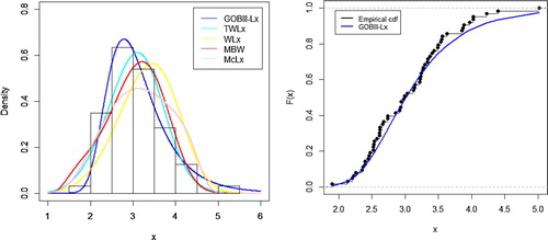
The estimates obtained from GOBIII-Lx distribution are considered better than all other fitted models as its accuracy measures are least. Also, the fitted density of GOBIII-Lx distribution is closer to the sample histogram and fitted cumulative distribution function is nearer to empirical cdf.

Data Set 2:

The second data set represents the remission times (in months) of a random sample of 128 bladder cancer patients as reported by [22]. We fit the above data sets by the GOBIII-W model along with the other well-known lifetime distributions namely; Kumaraswamy Weibull (Kw-W) [23], (BEW), (TEW), (BEE), beta modified Weibull (BMW) [24], and beta Weibull (BW) [25] distributions. The estimates and fitting measures are obtained by fitting different models to bladder cancer data and recorded in Table 5.

Table 5. MLEs (standard errors in parentheses) and goodness of fit statistics for bladder cancer data.

						Statistics
Model	Estimates					A	W
GOBIII-W (c,k,α,a,b)	2.2459215 (2.31901)	0.4106689 (0.13955)	4.349117 (1.17219)	0.3384453 (0.28274)	1.5331815 (2.0991)	0.20277	0.02672
Kw-W (δ,λ,α,β)	0.3222286 (0.25205)	0.540658 (0.368956)	2.3035236 (1.39464)	2.38848 (5.20245)	–	0.417858	0.06508
BEW (α,λ,γ,a,b,c)	2.3999 (3.364)	0.1799 (15.818)	0.550923 (0.243)	1.36362 (25.029)	2.13209 (3.079)	0.267495	0.040076
TEW (k,α,β,λ)	1.1333 (1.8985)	0.744922 (1.2456)	0.04784 (2.5871)	7.676E-10 (5.2142)	–	0.56339	0.08826
BEE (a,b,α,λ)	20.1471 (574.98)	15.0994 (0.01021)	0.141486 (37.768)	0.0031253 (0.14151)	–	0.34622	0.19917
BMW (α,γ,λ,a,b)	0.4697 (0.4788)	0.6661 (0.3123)	5.8×10–13 (0.0064)	2.7348 (2.0202)	0.9083 (1.522)	0.2719	0.0405
BW (a,b,γ,λ)	2.73477 (0.31749)	0.908258 (1.74023)	0.666132 (0.38549)	0.321567 (0.00795)	–	0.67549	0.117141

We find that the GOBIII-W distribution provides a better fit than six models. It has the smallest A and W values among those considered here. Plots of the fitted densities and the histogram and empirical cdfs are given in Figure 5.

Figure 5. (left) Plot of fitted densities superimposed on sample histogram. (right) empirical cdf and cdf of fitted GOBIII-W distribution.

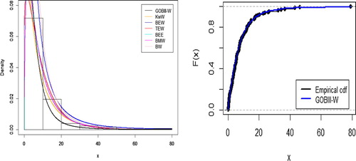
The estimates obtained from GOBIII-Lx distribution are considered better than all other fitted models as its accuracy measures are least. Also, the fitted density of GOBIII-Lx distribution is closer to the sample histogram and fitted cumulative distribution function is nearer to empirical cdf.

7. Conclusion

There has been rising interest among scientists in developing flexible lifetime models in order to improve the modelling of survival data. In this paper, we have proposed a new family of continuous distributions called generalized odd Burr III-G family of distributions. We have derived some mathematical properties of this proposed family along with its characterizations. The estimation of the unknown parameters of this family is approached by the method of maximum likelihood. We have presented real data applications to both skewed as well as symmetric data to illustrate the importance of the proposed family. Different special models of GOBIII family are used to fit real data sets and the results of these applications suggested that the new family provides consistently better fits for skewed and symmetric data sets. We hope that the newly proposed family of distributions may attract wider applications in survival analysis of all kind of types.

Disclosure statement

No potential conflict of interest was reported by the authors.

ORCID

Muhammad Ahsan ul Haq http://orcid.org/0000-0002-0902-8080

Sharqa Hashmi http://orcid.org/0000-0003-1824-7311

Appendix

Theorem A1:

Let X: $\mathrm{\Omega }\to \left(0,\mathrm{\infty }\right)$ be a continuous random variable with the distribution function F and let q1(x) and q2(x) be two real functions defined on H (let H = [d, e] be an interval for some d < e (d= -∞, e=∞ might as well be allowed)) such that $E\left[q_2\left(X\right)\text{|}X\ge x\right]=E\left[q_1\left(X\right)\text{|}X\ge x\right]\eta \left(x\right),xϵH$is defined with some real function η. Assume that $q_1,q_2ϵC^1\left(H\right),\eta ϵC^2\left(H\right)$ and F is twice continuously differentiable and strictly monotone function on the set H. Finally, assume that the equation $\eta q_1=q_2$ has no real solution in the interior of H. Then F is uniquely determined by the functions $q_1,q_2$ and $\eta$, particularly $F\left(x\right)=\text{C}{\int }_a^x\left|\frac{{\eta }^{\mathrm{\prime }}\left(u\right)}{\eta \left(u\right)q_1\left(u\right)-q_2\left(u\right)}\right|\exp \left(-s\left(u\right)\right)du,$where the function “s” is a solution of the differential equation $s^{\mathrm{\prime }}=\frac{{\eta }^{\mathrm{\prime }}{q}_1}{\eta q_1-q_2}$ and C is the normalization constant such that ${\int }_H^{}dF=1.$

This is the characterization.

Data set 1: 1.901, 2.132, 2.203, 2.228, 2.257, 2.350, 2.361, 2.396, 2.397, 2.445, 2.454, 2.474, 2.518, 2.522, 2.525, 2.532, 2.575, 2.614, 2.616, 2.618, 2.624, 2.659, 2.675, 2.738, 2.740, 2.856, 2.917, 2.928, 2.937, 2.937, 2.977, 2.996, 3.030, 3.125, 3.139, 3.145, 3.220, 3.223, 3.235, 3.243, 3.264, 3.272, 3.294, 3.332, 3.346, 3.377, 3.408, 3.435, 3.493, 3.501, 3.537, 3.554, 3.562, 3.628, 3.852, 3.871, 3.886, 3.971, 4.024, 4.027, 4.225, 4.395, 5.020.

Data set 2: 0.08, 2.09, 3.48, 4.87, 6.94, 8.66, 13.11, 23.63, 0.20, 2.23, 0.26, 0.31, 0.73, 0.52, 4.98, 6.97, 9.02, 13.29, 0.40, 2.26, 3.57, 5.06, 7.09, 11.98, 4.51, 2.07, 0.22, 13.8, 25.74, 0.50,2.46, 3.64, 5.09, 7.26, 9.47, 14.24, 19.13, 6.54, 3.36, 0.82, 0.51, 2.54, 3.70, 5.17, 7.28, 9.74, 14.76, 26.31, 0.81, 1.76, 8.53, 6.93, 0.62, 3.82, 5.32, 7.32, 10.06, 14.77, 32.15, 2.64, 3.88, 5.32, 3.25, 12.03, 8.65, 0.39, 10.34, 14.83, 34.26, 0.90,2.69, 4.18, 5.34, 7.59, 10.66, 4.50, 20.28, 12.63, 0.96, 36.66, 1.05, 2.69, 4.23, 5.41, 7.62, 10.75, 16.62, 43.01, 6.25, 2.02, 22.69, 0.19, 2.75, 4.26, 5.41, 7.63, 17.12, 46.12, 1.26, 2.83, 4.33, 8.37, 3.36, 5.49, 0.66, 11.25, 17.14, 79.05, 1.35, 2.87, 5.62, 7.87, 11.64, 17.36, 12.02, 6.76, 0.40, 3.02, 4.34, 5.71, 7.93, 11.79, 18.1, 1.46, 4.40, 5.85, 2.02, 12.07.

R Code for Application

rm(list=ls())

library(AdequacyModel)

data<-c(0.08, 2.09, 3.48, 4.87, 6.94, 8.66, 13.11, 23.63, 0.2, 2.23, 0.26, 0.31, 0.73, 0.52, 4.98, 6.97, 9.02, 13.29, 0.4, 2.26, 3.57, 5.06, 7.09, 11.98, 4.51, 2.07, 0.22, 13.8, 25.74, 0.5, 2.46, 3.64, 5.09, 7.26, 9.47, 14.24, 19.13, 6.54, 3.36, 0.82, 0.51, 2.54, 3.7, 5.17, 7.28, 9.74, 14.76, 26.31, 0.81, 1.76,8.53, 6.93, 0.62, 3.82, 5.32, 7.32, 10.06, 14.77, 32.15, 2.64, 3.88, 5.32, 3.25, 12.03, 8.65, 0.39, 10.34, 14.83, 34.26, 0.9, 2.69, 4.18, 5.34, 7.59, 10.66, 4.5, 20.28, 12.63, 0.96, 36.66, 1.05, 2.69, 4.23, 5.41, 7.62, 10.75, 16.62, 43.01, 6.25, 2.02, 22.69, 0.19, 2.75, 4.26, 5.41, 7.63, 17.12, 46.12, 1.26, 2.83, 4.33, 8.37, 3.36, 5.49, 0.66, 11.25, 17.14, 79.05, 1.35, 2.87, 5.62, 7.87, 11.64, 17.36, 12.02, 6.76, 0.4, 3.02, 4.34, 5.71, 7.93, 11.79, 18.1, 1.46, 4.4, 5.85, 2.02, 12.07)

• pdf_OBIIIW<- function(par,x){

• alpha=par[1]

• c=par[2]

• k=par[3]

• a=par[4]

• b=par[5]

• g= dweibull(x,a,b)

• G= pweibull(x,a,b)

• c*k*alpha*g*(((1-G^alpha)^(c-1))/(G^((c*alpha)+1)))*(1+((1-G^alpha)/G^alpha)^c)^(-k-1)

• }

• cdf_OBIIIW<- function(par,x){

• alpha=par[1]

• c=par[2]

• k=par[3]

• a=par[4]

• b=par[5]

• g= dweibull(x,a,b)

• G= pweibull(x,a,b)

• (1+((1-G^alpha)/G^alpha)^c)^(-k)

• }

• goodness.fit(pdf=pdf_OBIIIW, cdf=cdf_OBIIIW,starts = c(1,2,1,3,15),

• data,method=“S,” domain=c(0,Inf),mle=NULL)

References

- Eugene N, Lee C, Famoye F. Beta-normal distribution and its applications. Commun Stat Methods. 2002;31(4):497–512.
- Cordeiro GM, de Castro M. A new family of generalized distributions. J Stat Comput Simul. 2011;81(7):883–898.
- Marshall AW, Olkin I. A new method for adding a parameter to a family of distributions with application to the exponential and Weibull families. Biometrika. 1997;84(3):641–652.
- Alexander C, Cordeiro GM, Ortega EMM, et al. Generalized beta-generated distributions. Comput Stat Data Anal. 2012;56(6):1880–1897.
- Bourguignon M, Silva RB, Cordeiro GM. The Weibull-G family of probability distributions. J Data Sci. 2014;12:53–68.
- Cordeiro GM, Ortega EMM, Popović B V, et al. The Lomax generator of distributions: properties, minification process and regression model. Appl Math Comput. 2014;247:465–486.
- Soliman AH, Elgarhy MAE, Shakil M. Type II half logistic family of distributions with applications. Pak J Stat Oper Res. 2017;13(2):245–264.
- Elgarhy M, Haq MA, Özel G, et al. A new exponentiated extended family of distributions with applications. Gazi Univ J Sci. 2017;30(3):101–115.
- Haq MA, Elgarhy M. The odd Fréchet-G family of probability distributions. J Stat Appl Probab. 2018;7(1):189–203.
- Haq MA, Handique L, Chakraborty S. The odd moment exponential family of distributions: its properties and applications. Int J Appl Math Stat. 2018;57(6):47–62.
- Tahir MH, Nadarajah S. Parameter induction in continuous univariate distributions: well-established G families. An Acad Bras Cienc SciELO Brasil. 2015;87(2):539–568.
- Alzaatreh A, Lee C, Famoye F. A new method for generating families of continuous distributions. Metron. 2013;71(1):63–79.
- Jamal F, Nasir MA, Tahir MH, et al. The odd Burr-III family of distributions. J Stat Appl Pro. 2017;6(1):105–122.
- Glänzel W. A characterization theorem based on truncated moments and its application to some distribution families. Math Stat Probab Theory. 1987;B:75–84.
- Smith JL, Paul D, Paul R. No place for a woman: Evidence for gender bias in evaluations of presidential candidates. Basic Appl Soc Psych. 2007;29(3):225–233.
- Rényi A. On measures of entropy and information. Hung Acad Sci. 1961: 547–561.
- Kundu D, Raqab MZ. Estimation of R= P (Y< X) for three-parameter Weibull distribution. Stat Probab Lett. 2009;79(17):1839–1846.
- Afify AZ, Nofal ZM, Yousof HM, et al. The transmuted Weibull Lomax distribution: properties and application. Pak J Stat Oper Res. 2015;11(1):135–152.
- Khan MN. The modified beta Weibull distribution. Hacettepe J Math Stat. 2015;44:1553–1568.
- Lemonte AJ, Cordeiro GM. An extended Lomax distribution. Statistics (Ber). 2013;47(4):800–816.
- Tahir MH, Cordeiro GM, Mansoor M, et al. The Weibull-Lomax distribution: properties and applications. Hacettepe J Math Stat. 2015;44(2):461–480.
- Lee ET, Wang J. Statistical methods for survival data analysis. Vol. 476. Oklahoma: John Wiley & Sons; 2003.
- Cordeiro GM, Ortega EMM, Nadarajah S. The Kumaraswamy Weibull distribution with application to failure data. J Franklin Inst. 2010;347(8):1399–1429.
- Silva GO, Ortega EMM, Cordeiro GM. The beta modified Weibull distribution. Lifetime Data Anal. 2010;16(3):409–430.
- Lee C, Famoye F, Olumolade O. Beta-Weibull distribution: some properties and applications to censored data. J Mod Appl Stat Methods. 2007;6(1):17.
Appendix
Theorem A1:
Let X: be a continuous random variable with the distribution function F and let q1(x) and q2(x) be two real functions defined on H (let H = [d, e] be an interval for some d < e (d= -∞, e=∞ might as well be allowed)) such that
is defined with some real function η. Assume that
and F is twice continuously differentiable and strictly monotone function on the set H. Finally, assume that the equation
has no real solution in the interior of H. Then F is uniquely determined by the functions
and
, particularly
where the function “s” is a solution of the differential equation
and C is the normalization constant such that