Resolution of coincident factors in altering the flow dynamics of an MHD elastoviscous fluid past an unbounded upright channel

Abstract

The influence of simultaneous variation of slip and temperature has been inquired for the case of free-convected flow of an MHD (magnetohydrodynamic), elastoviscous fluid past an unbounded upright plate. How the course of velocity is revamped in response to temperature alterations on boundary has been studied by considering two cases of constant temperature and variable temperature. The inverse and direct role of elastoviscous parameter (K), thermal Grashof number ($G_r$) and Hartmann number (M) in determining the pattern of flow has been discussed through exact expressions and graphical illustrations. Interestingly, a $G_r$-regime has been identified corresponding to elastoviscous velocity variation. The Newtonian fluid velocity past an unbounded plate entailing slip factor has also been retrieved and compared with elastoviscous fluid velocity. This comparative analysis reflects on magnitude and profile adaptations in response to numerical changes.

Keywords:

• Elastoviscosity
• unsteady state
• free convection
• velocity
• temperature
• magnetic field

Mathematics Subject Classifications:

• 76D10
• 76R10
• 35Q79
• 65M38
• 44A10

1. Introduction

Heat transfer in free-convective flows has been vastly studied [1–4] keeping in view of its applications in manufacturing and chemical industries, food processing, therapeutic medicine, bio-engineering, hydro-energy saving, nuclear energy technologies and nuclear power processes, etc. A wide range of topics including the study of flows in mixed, hydromagnetic and laminar free convection, role of varying geometrical configurations on dynamics, preparation of colloidal particles by thermal decomposition, determination of thermal dose in cancer therapy, etc., were explored and compared. To develop the processes of isothermal chemical reactor and heating blocks using heat exchanger plate and heat sinks, heat convective flows past or in between vertical plates were studied.

Dynamics of fluid flowing past an upright oscillating were discussed with the help of closed analytical expressions for the first time by Soundalgekar [5,6]. Another dimension of studying combined effects of heat convection and magnetic conduction was explored, owing to its use in systemization such as regulating the temperature in intrinsic activator along with magnetic conduction and iron flow check in steel industry, etc. Mazumdar et al. [7] described an analytical method to study magnetohydrodynamic flow (MHD) past an impulsively started vertical channel. This work led by Deka et al. [8] and Khaleque et al. [9] to extend the probe of MHD convective flows past vertical channels to porous and stretching mediums. A multi-range applications of elastoviscous fluids flow in boundary overlay control problems in aerodynamics and biophysics have generated interest among researchers to investigate the dynamics of related systems and their stability. The comparable driving mechanism of flow in kidneys with elastoviscous fluid has also been another motivation to delve into the topic more explicitly. But due to complex nature of dynamical equations and difficulty in determining closed-form expressions corresponding to elastoviscous fluid flow, the dimension of concerned literature is restricted to comparatively simpler geometrical settings and numerical observations of flow pattern. A preliminary set of results regarding flow past an unbounded plate, both impulsively started and uniformly accelerated, accommodating heat convection and mass relegation were conferred in [10,11]. Singh et al. and Chen [12,13] made contributions to heat and mass transfer flow study, considering normal oscillating suction and convection adjacent to vertical surface. Flow behaviour of ionized gases through measuring Hall effects was reviewed by Achraya et al. and Aboeldahab et al. [14–16].

In addition to the study of free-convection flow with mass-heat deportation, many aspects of simple Newtonian and non-Newtonian fluids in different settings of channels have been recently documented reflecting on variation in behaviour of flow due to changes in shear stress or velocity boundary conditions [17–25]. Also, the effects of high temperature insulation and heat radiation in MHD nanofluids in porous medium were determined in [26,27]. Some interesting results were also added to the literature regarding studying the dynamics of fluids with varying viscosity through fractional derivative approach [28–31].

However, in all above-mentioned work, the dynamics of motion of fluid were discussed through only employing no-slip boundary conditions on velocity and shear stress and time-dependent shear application on channel. Also, among these were the results produced for dynamics of free-convection MHD flows with heat transfer with no-slip boundary condition on velocity. But due to complexity of governing equations, numerical simulation or fractional methodology was adopted, rendering the results to be perceived for ideal situation or away from real models. However, approximation of some parametric values in some cases led to exact analytical results matching those available in history [31,32]. More recently, some researchers have contributed a great deal towards exploration of MHD free-convecting fluids' dynamics in progressive empirical settings [33–42] using computational schemes. To the best of our knowledge, an MHD elastoviscous free-convective fluid flow past an unbounded channel/plate with slip and fluctuating temperature has not been studied before. The elastoviscous nature of some fluids in a boundary layer control scenario makes it imperative to study the flow characteristics of buoyancy and viscousness along with slip on the channel. The combined effects of slip, elasticity, temporal provision of temperature on boundary and magnetic field prevalence will be studied here to completely describe the dynamics of free-convection elastoviscous fluid flow.

In this work, we have analysed the free-convective, unsteady motion of an MHD elastoviscous fluid passing over an unbounded plate considering the factors of fluid slip on boundary and variable temperature. Rigorous expressions of temperature and velocity have been obtained using direct and inverse Laplace transform for two cases of supplying temperature to the boundary, unlike the fractional derivative approach [19,22,32] that confined the spectrum of region of solution due to fractional parameters' limitation. Due to complex nature of governing equations of elastoviscous fluid continuance, exact execution of velocity field has been spared in the literature in favour of numerical solutions. One of main advantages of our method, notwithstanding the cumbersome calculations and extremely long equations, is generation of these exact results that could always be referred for similar problems for veracity of computational results. For our problem, we have validated the numerical observations using exact expressions and graphical illustrations. The trappings of fluid criterion, i.e. Grashof number (thermal), $G_r$, Hartmann number, M, Prandtl number, $P_r$, and elastoviscous parameter, K, have been probed. Validation of our current results has also been achieved [18,25] by obtaining the solutions for Newtonian fluid, considering the limiting values of present fluid model's parameters.

2. Mathematical construction of the problem

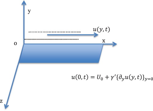
An MHD, elastoviscous fluid flow past an unbounded upstanding plate, along x-axis, is considered. Assuming that flow is along the vertical span of channel, which is normal to y-axis (Figure 1). At t = 0, resting position of plate is ensured, maintaining the temperature $T_{\mathrm{\infty }}$. In response to the administered motion $U_0$ of plate along with its contemporaneously raised temperature $T_W$, fluid initiates its propagation with slip at $t=0^{+}$. The unsteady mobility of convection-free slipping flow with wavering temperature is studied. Also, consistent magnetic conduction of strength $B_0$ is exercised normally to the plate. Compared with transverse magnetic range, an imperceptibility of magnetic field is observed. Reynolds number is assumed to hold least possible values. Keeping track of our model conditions, assumptions and Boussinesq approximation, the elastoviscous fluid flow is described by subsequent governing equations [43] (1) $\begin{array}{rl}\frac{\mathrm{\partial }u(y,t)}{\mathrm{\partial }t}& =\nu \frac{{\mathrm{\partial }}^{2}u(y,t)}{\mathrm{\partial }{y}^2}+g\text{β}\left(T\right(y,t)-T_{\mathrm{\infty }})\\ & +\frac{K^{\mathrm{\prime }}}{\rho }\frac{{\mathrm{\partial }}^{3}u(y,t)}{\mathrm{\partial }{y}^2\mathrm{\partial }t}-\frac{\sigma {B_0}^{2}u(y,t)}{\rho },\end{array}$(1) (2) $\begin{array}{rl}\frac{\mathrm{\partial }T(y,t)}{\mathrm{\partial }t}& =\frac{\kappa }{\rho C_p}\frac{{\mathrm{\partial }}^{2}T(y,t)}{\mathrm{\partial }{y}^2},\end{array}$(2) with conditions at t = 0 and y = 0, (3) $\begin{array}{rl}& u(y,0)=0,T(y,0)=T_{\mathrm{\infty }},y\in [0,\mathrm{\infty })\end{array}$(3) (4) $\begin{array}{rl}& u(0,t)=U_0+{\gamma }^{\mathrm{\prime }}\left\{{\mathrm{\partial }}_{y}u\right(y,t){\}}_{y=0},U\in (0,\mathrm{\infty })\end{array}$(4) (5) $\begin{array}{rl}& T(0,t)=T_W[1+af(t\left)\right]+T_{\mathrm{\infty }},t\in (0,\mathrm{\infty })\end{array}$(5) (6) $\begin{array}{rl}& u(y,t)\to 0,T(y,t)\to 0,\mathrm{f}\mathrm{o}\mathrm{r}y\to \mathrm{\infty }.\end{array}$(6) In above system, fluid velocity, density, its temperature, heat conduction, coefficient of heat expansion, electric conduction, constant-pressure specific heat, kinematic viscosity, elastoviscous coefficient and gravity acceleration are symbolized by $u(y,t)$, ρ, $T(y,t)$, κ, β, σ, $C_p$, ν, $K^{\mathrm{\prime }}$ and g, respectively. Also, ${\gamma }^{\mathrm{\prime }}$ and a are taken for constants. Equation (4(4) $\begin{array}{rl}& u(0,t)=U_0+{\gamma }^{\mathrm{\prime }}\left\{{\mathrm{\partial }}_{y}u\right(y,t){\}}_{y=0},U\in (0,\mathrm{\infty })\end{array}$(4) ) reflects on the aspect of slip between fluid and plate.

Figure 1. Geometry of flow.

We use the following non-dimensional variables to simplify our system (7) $\begin{array}{rl}{u}^{\ast }& =\frac{u}{U_0},y^{\ast }=\frac{y{U}_0}{\nu },t^{\ast }=\frac{t{U_0}^2}{\nu },T^{\ast }=\frac{T-T_{\mathrm{\infty }}}{T_W},\\ M& =\frac{\sigma B_0^2{\nu }^2}{\mu U_0^2},G_r=\frac{g\text{β}{T}_W\nu }{U_0^3},K=\frac{K^{\mathrm{\prime }}{U}_0^2}{\mu \nu },P_r=\frac{\mu C_p}{\kappa },\end{array}$(7) where K, M, $G_r$ and $P_r$ enumerate elastoviscosity, Hartmann, Grashof (heat) and Prandtl strength, respectively.

Using non-dimensional variables in Equation (7(7) $\begin{array}{rl}{u}^{\ast }& =\frac{u}{U_0},y^{\ast }=\frac{y{U}_0}{\nu },t^{\ast }=\frac{t{U_0}^2}{\nu },T^{\ast }=\frac{T-T_{\mathrm{\infty }}}{T_W},\\ M& =\frac{\sigma B_0^2{\nu }^2}{\mu U_0^2},G_r=\frac{g\text{β}{T}_W\nu }{U_0^3},K=\frac{K^{\mathrm{\prime }}{U}_0^2}{\mu \nu },P_r=\frac{\mu C_p}{\kappa },\end{array}$(7) ), our system becomes (dropping $\ast$) (8) $\begin{array}{rl}& \frac{\mathrm{\partial }u(y,t)}{\mathrm{\partial }t}=\frac{{\mathrm{\partial }}^{2}u(y,t)}{\mathrm{\partial }{y}^2}+G_{r}T(y,t)\\ & +K\frac{{\mathrm{\partial }}^{3}u(y,t)}{\mathrm{\partial }{y}^2\mathrm{\partial }t}-Mu(y,t),\end{array}$(8) (9) $\begin{array}{rl}& \frac{\mathrm{\partial }T(y,t)}{\mathrm{\partial }t}=\frac{1}{P_r}\frac{{\mathrm{\partial }}^{2}T(y,t)}{\mathrm{\partial }{y}^2},\end{array}$(9) (10) $\begin{array}{rl}& u(y,0)=T(y,0)=0,y\in [0,\mathrm{\infty })\end{array}$(10) (11) $\begin{array}{rl}& u(0,t)=1+\gamma \left\{{\mathrm{\partial }}_{y}u\right(y,t){\}}_{y=0},t\in (0,\mathrm{\infty })\end{array}$(11) (12) $\begin{array}{rl}& T(0,t)=1+af\left(t\right),t\in (0,\mathrm{\infty })\end{array}$(12) (13) $\begin{array}{rl}& u(y,t),T(y,t)\to 0,\mathrm{f}\mathrm{o}\mathrm{r}y\to \mathrm{\infty }.\end{array}$(13)

3. Mathematical solutions

Laplace transform of Equation (9(9) $\begin{array}{rl}& \frac{\mathrm{\partial }T(y,t)}{\mathrm{\partial }t}=\frac{1}{P_r}\frac{{\mathrm{\partial }}^{2}T(y,t)}{\mathrm{\partial }{y}^2},\end{array}$(9) ) is taken, in conjunction with conditions 10(10) $\begin{array}{rl}& u(y,0)=T(y,0)=0,y\in [0,\mathrm{\infty })\end{array}$(10) and (12(12) $\begin{array}{rl}& T(0,t)=1+af\left(t\right),t\in (0,\mathrm{\infty })\end{array}$(12) ), in order to determine exact formulation of fluid temperature, $T(y,t)$ (14) $\overline{T}(y,s)=(\frac{1}{s}+aF\left(s\right))e^{-\sqrt{P_{r}s}y}.$(14) Inverse application of Laplace on Equation (14(14) $\overline{T}(y,s)=(\frac{1}{s}+aF\left(s\right))e^{-\sqrt{P_{r}s}y}.$(14) ) delivers $\begin{array}{rl}T(y,t)& =erfc(\frac{\sqrt{P_r}y}{2\sqrt{t}})\\ & +\frac{a\sqrt{P_r}}{2}{\int }_0^{t}f(t-q)\frac{y}{\sqrt{\pi (q{)}^3}}{e}^{-\frac{P_r{y}^2}{4q}}\mathrm{d}q,\end{array}$ which in simple form is also given by (15) $\begin{array}{rl}T(y,t)& =erfc(\frac{\sqrt{P_r}y}{2\sqrt{t}})\\ & +\frac{2a}{\sqrt{\pi }}{\int }_{\frac{\sqrt{P_r}y}{2\sqrt{t}}}^{\mathrm{\infty }}f(t-\frac{P_r{y}^2}{4x^2})e^{-x^2}\mathrm{d}x,\end{array}$(15) meeting the conditions implied at initial time and on the boundary.

Now, Equation (8(8) $\begin{array}{rl}& \frac{\mathrm{\partial }u(y,t)}{\mathrm{\partial }t}=\frac{{\mathrm{\partial }}^{2}u(y,t)}{\mathrm{\partial }{y}^2}+G_{r}T(y,t)\\ & +K\frac{{\mathrm{\partial }}^{3}u(y,t)}{\mathrm{\partial }{y}^2\mathrm{\partial }t}-Mu(y,t),\end{array}$(8) ) is considered for the application of Laplace transform to obtain elastoviscous velocity field (16) $\overline{u}(y,s)=\frac{{\mathrm{\partial }}^2\overline{u}(y,s)}{\mathrm{\partial }{y}^2}+G_r\overline{T}(y,s)+Kq\frac{{\mathrm{\partial }}^2\overline{u}(y,s)}{\mathrm{\partial }{y}^2}-M\overline{u}(y,s).$(16)

Solving Equation (16(16) $\overline{u}(y,s)=\frac{{\mathrm{\partial }}^2\overline{u}(y,s)}{\mathrm{\partial }{y}^2}+G_r\overline{T}(y,s)+Kq\frac{{\mathrm{\partial }}^2\overline{u}(y,s)}{\mathrm{\partial }{y}^2}-M\overline{u}(y,s).$(16) ) using Laplace transform of Equations (11(11) $\begin{array}{rl}& u(0,t)=1+\gamma \left\{{\mathrm{\partial }}_{y}u\right(y,t){\}}_{y=0},t\in (0,\mathrm{\infty })\end{array}$(11) ), (13(13) $\begin{array}{rl}& u(y,t),T(y,t)\to 0,\mathrm{f}\mathrm{o}\mathrm{r}y\to \mathrm{\infty }.\end{array}$(13) ), (14(14) $\overline{T}(y,s)=(\frac{1}{s}+aF\left(s\right))e^{-\sqrt{P_{r}s}y}.$(14) ), we attain (17) $\begin{array}{rl}\overline{u}(y,s)& =\frac{e^{-\sqrt{\frac{M+s}{1+Ks}}y}}{s(1+\gamma \sqrt{\frac{M+s}{1+Ks}})}\\ & +\frac{G_r{e}^{-\sqrt{\frac{M+s}{1+Ks}}y}}{P_{r}Ks(1+\gamma \sqrt{\frac{M+s}{1+Ks}})\left[\right(s-\lambda {)}^2-\left(\sqrt{\tau }{)}^2\right]}\\ & +\frac{G_{r}aF\left(s\right)e^{-\sqrt{\frac{M+s}{1+Ks}}y}}{P_{r}K(1+\gamma \sqrt{\frac{M+s}{1+Ks}})\left[\right(s-\lambda {)}^2-\left(\sqrt{\tau }{)}^2\right]}\\ & +\frac{\gamma G_r{e}^{-\sqrt{\frac{M+s}{1+Ks}}y}}{\sqrt{s}\sqrt{P_r}K\left[\right(s-\lambda {)}^2-\left(\sqrt{\tau }{)}^2\right]}\\ & +\frac{\gamma G_{r}aF\left(s\right)\sqrt{P_r}\sqrt{s}{e}^{-\sqrt{\frac{M+s}{1+Ks}}y}}{P_{r}K\left[\right(s-\lambda {)}^2-\left(\sqrt{\tau }{)}^2\right]}\\ & -\frac{G_r{e}^{-\sqrt{P_{r}s}y}}{s{P}_{r}K\left[\right(s-\lambda {)}^2-\left(\sqrt{\tau }{)}^2\right]}\\ & -\frac{G_{r}aF\left(s\right)e^{-\sqrt{P_{r}s}y}}{P_{r}K\left[\right(s-\lambda {)}^2-\left(\sqrt{\tau }{)}^2\right]}.\end{array}$(17) To determine the Laplace inverse, Equation (17(17) $\begin{array}{rl}\overline{u}(y,s)& =\frac{e^{-\sqrt{\frac{M+s}{1+Ks}}y}}{s(1+\gamma \sqrt{\frac{M+s}{1+Ks}})}\\ & +\frac{G_r{e}^{-\sqrt{\frac{M+s}{1+Ks}}y}}{P_{r}Ks(1+\gamma \sqrt{\frac{M+s}{1+Ks}})\left[\right(s-\lambda {)}^2-\left(\sqrt{\tau }{)}^2\right]}\\ & +\frac{G_{r}aF\left(s\right)e^{-\sqrt{\frac{M+s}{1+Ks}}y}}{P_{r}K(1+\gamma \sqrt{\frac{M+s}{1+Ks}})\left[\right(s-\lambda {)}^2-\left(\sqrt{\tau }{)}^2\right]}\\ & +\frac{\gamma G_r{e}^{-\sqrt{\frac{M+s}{1+Ks}}y}}{\sqrt{s}\sqrt{P_r}K\left[\right(s-\lambda {)}^2-\left(\sqrt{\tau }{)}^2\right]}\\ & +\frac{\gamma G_{r}aF\left(s\right)\sqrt{P_r}\sqrt{s}{e}^{-\sqrt{\frac{M+s}{1+Ks}}y}}{P_{r}K\left[\right(s-\lambda {)}^2-\left(\sqrt{\tau }{)}^2\right]}\\ & -\frac{G_r{e}^{-\sqrt{P_{r}s}y}}{s{P}_{r}K\left[\right(s-\lambda {)}^2-\left(\sqrt{\tau }{)}^2\right]}\\ & -\frac{G_{r}aF\left(s\right)e^{-\sqrt{P_{r}s}y}}{P_{r}K\left[\right(s-\lambda {)}^2-\left(\sqrt{\tau }{)}^2\right]}.\end{array}$(17) ) is produced as (18) $\begin{array}{rl}\overline{u}(y,s)& =G_1(y,s)\frac{1}{s}+\frac{G_r}{P_{r}K}{G}_1(y,s)\frac{1}{s\left[\right(s-\lambda {)}^2-\left(\sqrt{\tau }{)}^2\right]}\\ & +\frac{G_{r}a}{P_{r}K}{G}_1(y,s)F\left(s\right)\frac{1}{\left[\right(s-\lambda {)}^2-\left(\sqrt{\tau }{)}^2\right]}\\ & +\frac{\gamma G_r}{\sqrt{P_r}K}{G}_1(y,s)\frac{1}{\sqrt{s}\left[\right(s-\lambda {)}^2-\left(\sqrt{\tau }{)}^2\right]}\\ & +\frac{\gamma G_{r}a}{\sqrt{P_r}K}{G}_1(y,s)F\left(s\right)\frac{\sqrt{s}}{\left[\right(s-\lambda {)}^2-\left(\sqrt{\tau }{)}^2\right]}\\ & -\frac{G_r}{P_{r}K}\frac{e^{-\sqrt{P_r}y\sqrt{s}}}{s}\frac{1}{\left[\right(s-\lambda {)}^2-\left(\sqrt{\tau }{)}^2\right]}\\ & -\frac{G_{r}a}{P_{r}K}{e}^{-\sqrt{P_r}y\sqrt{s}}F\left(s\right)\frac{1}{\left[\right(s-\lambda {)}^2-\left(\sqrt{\tau }{)}^2\right]},\end{array}$(18) where $\begin{array}{rl}{G}_1(y,s)& =\frac{e^{-\sqrt{\frac{M+s}{1+Ks}}y}}{\gamma (\sqrt{\frac{M+s}{1+Ks}}+\frac{1}{\gamma })},\\ \tau & =(\frac{1-P_r}{2P_{r}K}{)}^2+\frac{M}{P_{r}K},\lambda =\frac{1-P_r}{2P_{r}K}.\end{array}$ Equation (18(18) $\begin{array}{rl}\overline{u}(y,s)& =G_1(y,s)\frac{1}{s}+\frac{G_r}{P_{r}K}{G}_1(y,s)\frac{1}{s\left[\right(s-\lambda {)}^2-\left(\sqrt{\tau }{)}^2\right]}\\ & +\frac{G_{r}a}{P_{r}K}{G}_1(y,s)F\left(s\right)\frac{1}{\left[\right(s-\lambda {)}^2-\left(\sqrt{\tau }{)}^2\right]}\\ & +\frac{\gamma G_r}{\sqrt{P_r}K}{G}_1(y,s)\frac{1}{\sqrt{s}\left[\right(s-\lambda {)}^2-\left(\sqrt{\tau }{)}^2\right]}\\ & +\frac{\gamma G_{r}a}{\sqrt{P_r}K}{G}_1(y,s)F\left(s\right)\frac{\sqrt{s}}{\left[\right(s-\lambda {)}^2-\left(\sqrt{\tau }{)}^2\right]}\\ & -\frac{G_r}{P_{r}K}\frac{e^{-\sqrt{P_r}y\sqrt{s}}}{s}\frac{1}{\left[\right(s-\lambda {)}^2-\left(\sqrt{\tau }{)}^2\right]}\\ & -\frac{G_{r}a}{P_{r}K}{e}^{-\sqrt{P_r}y\sqrt{s}}F\left(s\right)\frac{1}{\left[\right(s-\lambda {)}^2-\left(\sqrt{\tau }{)}^2\right]},\end{array}$(18) ) is considered for the application of inverse Laplace transform, in conjunction with Appendix (A1(25) $\begin{array}{rl}& \times [e^{y\sqrt{M+\mathrm{\Omega }}}erfc(\frac{y}{2\sqrt{t}}+\sqrt{(M+\mathrm{\Omega })t})\\ & \times +e^{-y\sqrt{M+\mathrm{\Omega }}}erfc(\frac{y}{2\sqrt{t}}-\sqrt{(M+\mathrm{\Omega })t})]\\ & +\frac{G_r{e}^{bt}}{2\gamma \mathrm{\Omega }(P_r-1)[1-{\gamma }^2(M+\mathrm{\Omega }\left)\right]\sqrt{M+\mathrm{\Omega }}}\\ & \times [e^{y\sqrt{M+\mathrm{\Omega }}}erfc(\frac{y}{2\sqrt{t}}+\sqrt{(M+\mathrm{\Omega })t})\\ & \times -e^{-y\sqrt{M+\mathrm{\Omega }}}erfc(\frac{y}{2\sqrt{t}}-\sqrt{(M+\mathrm{\Omega })t})]\\ & +\frac{G_r\sqrt{P_r}{e}^{\mathrm{\Omega }t}}{(P_r-1)\sqrt{\mathrm{\Omega }}}{\int }_0^t\{\frac{e^{-\frac{y^2}{4s}-(M+\mathrm{\Omega })s}}{\sqrt{\pi s}}erf\left(\sqrt{\mathrm{\Omega }(t-s)}\right)\\ & \times -\frac{1}{\gamma }{e}^{\frac{y}{\gamma }+\frac{s}{{\gamma }^2}-(M+\mathrm{\Omega })s}erfc(\frac{y}{2\sqrt{s}}+\frac{\sqrt{s}}{\gamma })\\ & \times erf\left(\sqrt{\mathrm{\Omega }(t-s)}\right)\}\mathrm{d}s\\ & -\frac{G_r{e}^{\mathrm{\Omega }t}}{2\mathrm{\Omega }(P_r-1)}[e^{y\sqrt{\mathrm{\Omega }{P}_r}}erfc(\frac{\sqrt{P_r}y}{2\sqrt{t}}+\sqrt{\mathrm{\Omega }t})\\ & \times +e^{-y\sqrt{\mathrm{\Omega }{P}_r}}erfc(\frac{\sqrt{P_r}y}{2\sqrt{t}}-\sqrt{\mathrm{\Omega }t})]\\ & +\frac{G_r}{\mathrm{\Omega }(P_r-1)}erf(\frac{\sqrt{P_r}y}{2\sqrt{t}}).\end{array}$(25) )–(A10(A6) $\begin{array}{rl}& {\mathcal{L}}^{-1}\{\frac{e^{-p\sqrt{s}}}{s}\}=erfc(\frac{p}{2\sqrt{t}}),\end{array}$(A6) ), to derive elastoviscous velocity (19) $\begin{array}{rl}& u(y,t)\\ & ={\int }_0^t{g}_1(y,q)\mathrm{d}q+\frac{G_r}{P_{r}K({\lambda }^2-\tau )}{\int }_0^t{g}_1(y,q)\mathrm{d}q\\ & +\frac{G_r}{P_{r}K(2\lambda \sqrt{\tau }+2\tau )}{\int }_0^t{g}_1(y,q)e^{(\lambda +\sqrt{\tau })(t-q)}\mathrm{d}q\\ & +\frac{G_r}{P_{r}K(2\tau -2\lambda \sqrt{\tau })}{\int }_0^t{g}_1(y,q)e^{(\lambda -\sqrt{\tau })(t-q)}\mathrm{d}s\\ & +\frac{G_{r}a}{2P_{r}K\sqrt{\tau }}{\int }_0^t{g}_1(y,q)H_1(t-q)\mathrm{d}q\\ & -\frac{G_{r}a}{2P_{r}K\sqrt{\tau }}{\int }_0^t{g}_1(y,q)H_2(t-q)\mathrm{d}q\\ & +\frac{\gamma G_r}{2K\sqrt{\tau P_r(\lambda +\sqrt{\tau })}}\\ & \times {\int }_0^t{g}_1(y,q)e^{(\lambda +\sqrt{\tau })(t-q)}\\ & \times erf\left(\sqrt{(\lambda +\sqrt{\tau })(t-q)}\right)\mathrm{d}q\\ & -\frac{\gamma G_r}{2K\sqrt{\tau P_r(\lambda -\sqrt{\tau })}}{\int }_0^t{g}_1(y,q)e^{(\lambda -\sqrt{\tau })(t-q)}\\ & \times erf\left(\sqrt{(\lambda -\sqrt{\tau })(t-q)}\right)\mathrm{d}q\\ & +\frac{\gamma G_{r}a}{2K\sqrt{\tau P_r}}{\int }_0^t{g}_1(y,q)R_1(t-q)\mathrm{d}q\\ & -\frac{\gamma G_{r}a}{2K\sqrt{\tau P_r}}{\int }_0^t{g}_1(y,q)R_2(t-q)\mathrm{d}q-\frac{G_r}{2K{P}_r\sqrt{\tau }}{\int }_0^t\\ & \times erfc(\frac{\sqrt{P_r}y}{2\sqrt{q}})e^{(\lambda +\sqrt{\tau })(t-q)}\mathrm{d}q\\ & +\frac{G_r}{2K{P}_r\sqrt{\tau }}{\int }_0^{t}erfc(\frac{\sqrt{P_r}y}{2\sqrt{q}})e^{(\lambda -\sqrt{\tau })(t-q)}\mathrm{d}q\\ & -\frac{G_{r}a}{2K{P}_r\sqrt{\tau }}{\int }_0^t\xi (t-q)f\left(q\right)\mathrm{d}q\\ & +\frac{G_{r}a}{2K{P}_r\sqrt{\tau }}{\int }_0^t\psi (t-q)f\left(q\right)\mathrm{d}q,\end{array}$(19) where $\begin{array}{rl}{g}_1(y,t)& ={\mathcal{L}}^{-1}\{G_1(y,s)\}={\mathcal{L}}^{-1}\{\left(F_{1}oQ\right)\left(s\right)\}\\ & ={\mathcal{L}}^{-1}\{F_1\left(Q\right(s\left)\right)\}={\int }_0^{\mathrm{\infty }}{f}_1(y,p)r(p,t)\mathrm{d}p,\\ f_1(y,t)& ={\mathcal{L}}^{-1}\left\{F_1\right(y,s\left)\right\}={\mathcal{L}}^{-1}\{\frac{e^{-\sqrt{s}y}}{\gamma (\sqrt{s}+\frac{1}{\gamma })}\}\\ & =\frac{1}{\gamma }\{\frac{e^{-\frac{y^2}{4t}}}{\sqrt{\pi t}}-\frac{1}{\gamma }{e}^{\frac{y}{\gamma }+\frac{t}{{\gamma }^2}}erfc(\frac{y}{2\sqrt{t}}+\frac{\sqrt{t}}{\gamma })\},\\ Q\left(s\right)& =\frac{M+s}{1-Ks},r(p,t)={\mathcal{L}}^{-1}\{e^{-zQ\left(s\right)}\}\\ & =e^{\frac{z}{K}}[\sqrt{\frac{\mathcal{O}}{t}}{I}_1\left(2\sqrt{\mathcal{O}}t\right)e^{\frac{t}{K}}+\delta \left(t\right)],\end{array}$

(Here first kind of order 1 modified Bessel function and delta function are taken to be as $I_1$ and $\delta \left(t\right)$, respectively. Also, $\mathcal{O}=\frac{z(MK+1)}{K^2}.$) $\begin{array}{rl}{H}_1\left(t\right)& ={\mathcal{L}}^{-1}\{\frac{F\left(s\right)}{s-(\lambda +\sqrt{\tau })}\}={\int }_0^{t}f\left(q\right)e^{(\lambda +\sqrt{\tau })(t-q)}\mathrm{d}q,\\ H_2\left(t\right)& ={\mathcal{L}}^{-1}\{\frac{F\left(s\right)}{s-(\lambda -\sqrt{\tau })}\}={\int }_0^{t}f\left(q\right)e^{(\lambda -\sqrt{\tau })(t-q)}\mathrm{d}q,\\ R_1\left(t\right)& ={\mathcal{L}}^{-1}\{F\left(s\right)\frac{\sqrt{s}}{s-(\sqrt{\lambda +\sqrt{\tau }}{)}^2}\}\\ & ={\int }_0^{t}f\left(q\right)[\frac{1}{\sqrt{\pi (t-q)}}+\sqrt{\lambda +\sqrt{\tau }}{e}^{(\lambda +\sqrt{\tau })(t-q)}\\ & \times erf(\sqrt{(\lambda +\sqrt{\tau })(t-q)}]\mathrm{d}q,\\ R_2\left(t\right)& ={\mathcal{L}}^{-1}\{F\left(s\right)\frac{\sqrt{s}}{s-(\sqrt{\lambda -\sqrt{\tau }}{)}^2}\}\\ & ={\int }_0^{t}f\left(q\right)[\frac{1}{\sqrt{\pi (t-q)}}+\sqrt{\lambda -\sqrt{\tau }}{e}^{(\lambda -\sqrt{\tau })(t-q)}\\ & \times erf(\sqrt{(\lambda -\sqrt{\tau })(t-q)}]\mathrm{d}q,\\ \xi \left(t\right)& ={\mathcal{L}}^{-1}\{\frac{e^{-\sqrt{P_r}y\sqrt{s}}}{s-(\lambda +\sqrt{\tau })}\}\\ & ={\int }_0^t\frac{\sqrt{P_r}y{e}^{-\frac{P_r{y}^2}{4u}}}{2u\sqrt{\pi u}}{e}^{(\lambda +\sqrt{\tau })(t-u)}\mathrm{d}u\\ & =\frac{\sqrt{P_r}{e}^{(\lambda +\sqrt{\tau })t}}{2}\left[e^{y\sqrt{P_r(\lambda +\sqrt{\tau })}}\right.\\ & \times erfc\left(\frac{\sqrt{P_r}y}{2\sqrt{t}}+\sqrt{(\lambda +\sqrt{\tau })t}\right)+e^{-y\sqrt{P_r(\lambda +\sqrt{\tau })}}\\ & \times \left.erfc\left(\frac{\sqrt{P_r}y}{2\sqrt{t}}-\sqrt{(\lambda +\sqrt{\tau })t}\right)\right],\\ \psi \left(t\right)& ={\mathcal{L}}^{-1}\{\frac{e^{-\sqrt{P_r}y\sqrt{s}}}{s-(\lambda -\sqrt{\tau })}\}\\ & ={\int }_0^t\frac{\sqrt{P_r}y{e}^{-\frac{P_r{y}^2}{4u}}}{2u\sqrt{\pi u}}{e}^{(\lambda -\sqrt{\tau })(t-u)}\mathrm{d}u\\ & =\frac{\sqrt{P_r}{e}^{(\lambda -\sqrt{\tau })t}}{2}\left[e^{y\sqrt{P_r(\lambda -\sqrt{\tau })}}\right.\\ & \times erfc\left(\frac{\sqrt{P_r}y}{2\sqrt{t}}+\sqrt{(\lambda -\sqrt{\tau })t}\right)\\ & \left.+e^{-y\sqrt{P_r(\lambda -\sqrt{\tau })}}erfc\left(\frac{\sqrt{P_r}y}{2\sqrt{t}}-\sqrt{(\lambda -\sqrt{\tau })t}\right)\right].\end{array}$

4. Limiting cases

Here, Newtonian fluid velocity expressions are obtained with and without magnetic field application. The responses of Newtonian fluid corresponding to constant temperature on boundary and elastoviscous fluid corresponding to constant velocity on boundary have also been recorded. These cases are

4.1. Newtonian fluid

For K to be very small (Equation 8(8) $\begin{array}{rl}& \frac{\mathrm{\partial }u(y,t)}{\mathrm{\partial }t}=\frac{{\mathrm{\partial }}^{2}u(y,t)}{\mathrm{\partial }{y}^2}+G_{r}T(y,t)\\ & +K\frac{{\mathrm{\partial }}^{3}u(y,t)}{\mathrm{\partial }{y}^2\mathrm{\partial }t}-Mu(y,t),\end{array}$(8) ), the model for elastoviscous fluid reduces to Newtonian fluid system. Equation (16(16) $\overline{u}(y,s)=\frac{{\mathrm{\partial }}^2\overline{u}(y,s)}{\mathrm{\partial }{y}^2}+G_r\overline{T}(y,s)+Kq\frac{{\mathrm{\partial }}^2\overline{u}(y,s)}{\mathrm{\partial }{y}^2}-M\overline{u}(y,s).$(16) ) becomes (20) $\begin{array}{rl}\overline{u}(y,s)& =\frac{e^{-\sqrt{s+M}y}}{s(1+\gamma \sqrt{s+M})}\\ & +\frac{G_r{e}^{-\sqrt{s+M}y}}{s(1+\gamma \sqrt{s+M})\left[\right(P_r-1)s-M]}\\ & +\frac{G_{r}aF\left(s\right)e^{-\sqrt{s+M}y}}{(1+\gamma \sqrt{s+M})\left[\right(P_r-1)s-M]}\\ & +\frac{\gamma G_r\sqrt{P_r}{e}^{-\sqrt{s+M}y}}{\sqrt{s}(1+\gamma \sqrt{s+M})\left[\right(P_r-1)s-M]}\\ & +\frac{\eta G_{r}aF\left(s\right)\sqrt{P_{r}s}{e}^{-\sqrt{s+M}y}}{(1+\gamma \sqrt{s+M})\left[\right(P_r-1)s-M]}\\ & -\frac{G_r{e}^{-\sqrt{P_{r}s}y}}{s\left[\right(P_r-1)s-M]}\\ & -\frac{G_{r}aF\left(s\right)e^{-\sqrt{P_{r}q}y}}{\left[\right(P_r-1)s-M]}.\end{array}$(20) Equation (20(20) $\begin{array}{rl}\overline{u}(y,s)& =\frac{e^{-\sqrt{s+M}y}}{s(1+\gamma \sqrt{s+M})}\\ & +\frac{G_r{e}^{-\sqrt{s+M}y}}{s(1+\gamma \sqrt{s+M})\left[\right(P_r-1)s-M]}\\ & +\frac{G_{r}aF\left(s\right)e^{-\sqrt{s+M}y}}{(1+\gamma \sqrt{s+M})\left[\right(P_r-1)s-M]}\\ & +\frac{\gamma G_r\sqrt{P_r}{e}^{-\sqrt{s+M}y}}{\sqrt{s}(1+\gamma \sqrt{s+M})\left[\right(P_r-1)s-M]}\\ & +\frac{\eta G_{r}aF\left(s\right)\sqrt{P_{r}s}{e}^{-\sqrt{s+M}y}}{(1+\gamma \sqrt{s+M})\left[\right(P_r-1)s-M]}\\ & -\frac{G_r{e}^{-\sqrt{P_{r}s}y}}{s\left[\right(P_r-1)s-M]}\\ & -\frac{G_{r}aF\left(s\right)e^{-\sqrt{P_{r}q}y}}{\left[\right(P_r-1)s-M]}.\end{array}$(20) ) is produced as given below, more suitable for inverse Laplace transform application (21) $\begin{array}{rl}\overline{u}(y,s)& =\frac{e^{-\sqrt{s+M}y}}{\gamma (\sqrt{s+M}+\frac{1}{\gamma })}\frac{1}{s}+\frac{G_r}{(P_r-1)}\\ & \times \frac{e^{-\sqrt{s+M}y}}{(\sqrt{s+M}+\frac{1}{\gamma })}\frac{1}{s(s-\mathrm{\Omega })}+\frac{G_{r}a}{\gamma (P_r-1)}\\ & \times \frac{e^{-\sqrt{s+M}y}}{\gamma (\sqrt{s+M}+\frac{1}{\gamma })}F\left(s\right)\frac{1}{s-\mathrm{\Omega }}\\ & +\frac{\gamma G_r\sqrt{P_r}}{(P_r-1)}\frac{e^{-\sqrt{s+M}y}}{\gamma (\sqrt{s+M}+\frac{1}{\gamma })}\frac{1}{\sqrt{s}(s-\mathrm{\Omega })}\\ & +\frac{\gamma G_{r}a\sqrt{P_r}}{(P_r-1)}\frac{e^{-\sqrt{s+M}y}}{\gamma (\sqrt{s+M}+\frac{1}{\gamma })}F\left(q\right)\frac{\sqrt{s}}{s-\mathrm{\Omega }}\\ & -\frac{G_r}{(P_r-1)}\frac{e^{-\sqrt{P_{r}s}y}}{s}\frac{1}{s-\mathrm{\Omega }}\\ & -\frac{G_{r}a}{(P_r-1)}{e}^{-\sqrt{P_{r}s}y}\frac{F\left(s\right)}{s-\mathrm{\Omega }},\end{array}$(21) where $\mathrm{\Omega }=\frac{M}{P_r-1}.$

Inverse application of Laplace on Equation (21(21) $\begin{array}{rl}\overline{u}(y,s)& =\frac{e^{-\sqrt{s+M}y}}{\gamma (\sqrt{s+M}+\frac{1}{\gamma })}\frac{1}{s}+\frac{G_r}{(P_r-1)}\\ & \times \frac{e^{-\sqrt{s+M}y}}{(\sqrt{s+M}+\frac{1}{\gamma })}\frac{1}{s(s-\mathrm{\Omega })}+\frac{G_{r}a}{\gamma (P_r-1)}\\ & \times \frac{e^{-\sqrt{s+M}y}}{\gamma (\sqrt{s+M}+\frac{1}{\gamma })}F\left(s\right)\frac{1}{s-\mathrm{\Omega }}\\ & +\frac{\gamma G_r\sqrt{P_r}}{(P_r-1)}\frac{e^{-\sqrt{s+M}y}}{\gamma (\sqrt{s+M}+\frac{1}{\gamma })}\frac{1}{\sqrt{s}(s-\mathrm{\Omega })}\\ & +\frac{\gamma G_{r}a\sqrt{P_r}}{(P_r-1)}\frac{e^{-\sqrt{s+M}y}}{\gamma (\sqrt{s+M}+\frac{1}{\gamma })}F\left(q\right)\frac{\sqrt{s}}{s-\mathrm{\Omega }}\\ & -\frac{G_r}{(P_r-1)}\frac{e^{-\sqrt{P_{r}s}y}}{s}\frac{1}{s-\mathrm{\Omega }}\\ & -\frac{G_{r}a}{(P_r-1)}{e}^{-\sqrt{P_{r}s}y}\frac{F\left(s\right)}{s-\mathrm{\Omega }},\end{array}$(21) ) and employing Appendix (A3(27) $\begin{array}{rl}\overline{u}(y,s)& =Z_1(y,s)\frac{1}{s}+\frac{G_r}{P_{r}K}{Z}_1(y,s)\frac{1}{s\left[\right(s-\lambda {)}^2-\left(\sqrt{\tau }{)}^2\right]}\\ & +\frac{G_{r}a}{P_{r}K}{Z}_1(y,s)F\left(s\right)\frac{1}{\left[\right(s-\lambda {)}^2-\left(\sqrt{\tau }{)}^2\right]}\\ & -\frac{G_r}{P_{r}K}\frac{e^{-\sqrt{P_r}y\sqrt{s}}}{s}\frac{1}{\left[\right(s-\lambda {)}^2-\left(\sqrt{\tau }{)}^2\right]}\\ & -\frac{G_{r}a}{P_{r}K}{e}^{-\sqrt{P_r}y\sqrt{s}}F\left(q\right)\frac{1}{\left[\right(s-\lambda {)}^2-\left(\sqrt{\tau }{)}^2\right]},\end{array}$(27) ), (A5(A1) $\begin{array}{rl}& \frac{1}{(s-\lambda {)}^2-(\sqrt{\tau }{)}^2}=\frac{1}{2\sqrt{\tau }}\frac{1}{s-(\lambda +\sqrt{\tau })}-\frac{1}{2\sqrt{\tau }}\frac{1}{s-(\lambda -\sqrt{\tau })},\end{array}$(A1) ), (A6(A2) $\begin{array}{rl}& \frac{1}{s\left[\right(s-\lambda {)}^2-\left(\sqrt{\tau }{)}^2\right]}=\frac{1}{({\lambda }^2-\tau )}\frac{1}{s}+\frac{1}{(2\lambda \sqrt{\tau }+2\tau )}\\ & \times \frac{1}{s-(\lambda +\sqrt{\tau })}+\frac{1}{(2\tau -2\lambda \sqrt{\tau })}\frac{1}{s-(\lambda -\sqrt{\tau })},\end{array}$(A2) ), we arrive at (22) $\begin{array}{rl}& u(y,t)=\frac{-\left[\mathrm{\Omega }\right(P_r-1)-G_r]}{2\gamma \mathrm{\Omega }(P_r-1)\sqrt{M}}[e^{y\sqrt{M}}erfc(\frac{y}{2\sqrt{t}}+\sqrt{Mt})\\ & -e^{-y\sqrt{M}}erfc(\frac{y}{2\sqrt{t}}-\sqrt{Mt})]\\ & -\frac{\left[\mathrm{\Omega }\right(P_r-1)-G_r]}{\mathrm{\Omega }(P_r-1)(1-{\gamma }^{2}M)}erfc(\frac{y}{2\sqrt{t}}+\frac{\sqrt{t}}{\gamma })\\ & e^{-Mt+\frac{t}{{\gamma }^2}+\frac{y}{\gamma }}\\ & -\frac{G_r{e}^{\mathrm{\Omega }t}}{\mathrm{\Omega }(P_r-1)[1-{\gamma }^2(M+\mathrm{\Omega }\left)\right]}\\ & \times erfc(\frac{y}{2\sqrt{t}}+\frac{\sqrt{t}}{\gamma })e^{Mt+\frac{t}{{\gamma }^2}+\frac{y}{\gamma }}\\ & +\frac{\left[\mathrm{\Omega }\right(P_r-1)-G_r]}{2\mathrm{\Omega }(P_r-1)(1-{\gamma }^{2}M)}[e^{y\sqrt{M}}erfc(\frac{y}{2\sqrt{t}}+\sqrt{Mt})\\ & -e^{-y\sqrt{M}}erfc(\frac{y}{2\sqrt{t}}-\sqrt{Mt})]\\ & -\frac{G_r{e}^{\mathrm{\Omega }t}}{2\gamma \mathrm{\Omega }(P_r-1)\sqrt{M+\mathrm{\Omega }}}[e^{y\sqrt{M+b}}\\ & \times erfc(\frac{y}{2\sqrt{t}}+\sqrt{(M+\mathrm{\Omega })t})\\ & -e^{-y\sqrt{M+b}}erfc(\frac{y}{2\sqrt{t}}-\sqrt{(M+\mathrm{\Omega })t})]\\ & +\frac{G_r{e}^{\mathrm{\Omega }t}}{2\mathrm{\Omega }(P_r-1)[1-{\gamma }^2(M+\mathrm{\Omega }\left)\right]}\\ & \times [e^{y\sqrt{M+\mathrm{\Omega }}}erfc(\frac{y}{2\sqrt{t}}+\sqrt{(M+\mathrm{\Omega })t})+e^{-y\sqrt{M+\mathrm{\Omega }}}\end{array}$(22) (22) $\begin{array}{rl}& \times erfc(\frac{y}{2\sqrt{t}}-\sqrt{(M+\mathrm{\Omega })t})]\\ & +\frac{G_r{e}^{bt}}{2\gamma \mathrm{\Omega }(P_r-1)[1-{\gamma }^2(M+b\left)\right]\sqrt{M+\mathrm{\Omega }}}\\ & \times [e^{y\sqrt{M+\mathrm{\Omega }}}erfc(\frac{y}{2\sqrt{t}}+\sqrt{(M+\mathrm{\Omega })t})\\ & -e^{-y\sqrt{M+b}}erfc(\frac{y}{2\sqrt{t}}-\sqrt{(M+b)t})]\\ & +\frac{G_r\sqrt{P_r}{e}^{\mathrm{\Omega }t}}{(P_r-1)\sqrt{\mathrm{\Omega }}}{\int }_0^t\{\frac{e^{-\frac{y^2}{4s}-(M+\mathrm{\Omega })s}}{\sqrt{\pi s}}erf\left(\sqrt{\mathrm{\Omega }(t-s)}\right)\\ & -\frac{1}{\gamma }{e}^{\frac{y}{\gamma }+\frac{s}{{\gamma }^2}-(M+\mathrm{\Omega })s}erfc(\frac{y}{2\sqrt{s}}+\frac{\sqrt{s}}{\gamma })\\ & \times erf\left(\sqrt{\mathrm{\Omega }(t-s)}\right)\}\mathrm{d}s\\ & +\frac{G_{r}a}{\gamma (P_r-1)}{\int }_0^t\{\frac{e^{-\frac{y^2}{4s}-Ms}}{\sqrt{\pi s}}-\frac{1}{\gamma }{e}^{\frac{y}{\gamma }+\frac{s}{{\gamma }^2}-Ms}\\ & \times erfc(\frac{y}{2\sqrt{s}}+\frac{\sqrt{s}}{\gamma })\}{H}_3(t-s)\mathrm{d}s\\ & +\frac{G_{r}a\sqrt{P_r}}{(P_r-1)}{\int }_0^t\{\frac{e^{-\frac{y^2}{4s}-Ms}}{\sqrt{\pi s}}-\frac{1}{\gamma }{e}^{\frac{y}{\gamma }+\frac{s}{{\gamma }^2}-Ms}\\ & \times erfc(\frac{y}{2\sqrt{s}}+\frac{\sqrt{s}}{\gamma })\}{R}_3(t-s)\mathrm{d}s\\ & -\frac{G_r{e}^{\mathrm{\Omega }t}}{2\mathrm{\Omega }(P_r-1)}[e^{y\sqrt{\mathrm{\Omega }{P}_r}}erfc(\frac{\sqrt{P_r}y}{2\sqrt{t}}+\sqrt{\mathrm{\Omega }t})\\ & +e^{-y\sqrt{\mathrm{\Omega }{P}_r}}erfc(\frac{\sqrt{P_r}y}{2\sqrt{t}}-\sqrt{\mathrm{\Omega }t})]\\ & +\frac{G_r}{\mathrm{\Omega }(P_r-1)}erf(\frac{\sqrt{P_r}y}{2\sqrt{t}})-\frac{G_{r}a\sqrt{P_r}y}{2(P_r-1)\sqrt{\pi }}\\ & \times {\int }_0^t\frac{e^{\frac{-P_r{y}^2}{4s}}}{\sqrt{s^3}}{H}_3(t-s)\mathrm{d}s.\end{array}$(22)

4.2. Absence of magnetic field ($M\to 0$)

Considering a frame devoid of magnetic occupation ($M\to 0$) for Newtonian fluid ($K\to 0$), the expression for velocity has been computed as (23) $\begin{array}{rl}& u(y,t)=\frac{-2\left[\mathrm{\Omega }\right(P_r-1)-G_r]}{\gamma \mathrm{\Omega }(P_r-1)}\{yerfc(\frac{y}{2\sqrt{t}})-\sqrt{t}{e}^{\frac{-y^2}{4t}}\}\\ & -\frac{\left[\mathrm{\Omega }\right(P_r-1)-G_r]}{\mathrm{\Omega }(P_r-1)}erfc(\frac{y}{2\sqrt{t}}+\frac{\sqrt{t}}{\gamma })e^{\frac{t}{{\gamma }^2}+\frac{y}{\gamma }}\\ & +\frac{\left[\mathrm{\Omega }\right(P_r-1)-G_r]}{\mathrm{\Omega }(P_r-1)}erfc(\frac{y}{2\sqrt{t}})\\ & -\frac{G_r{e}^{\mathrm{\Omega }t}}{\mathrm{\Omega }(P_r-1)(1-{\gamma }^2\mathrm{\Omega })}erfc(\frac{y}{2\sqrt{t}}+\frac{\sqrt{t}}{\gamma })e^{-\mathrm{\Omega }t+\frac{t}{{\gamma }^2}+\frac{y}{\gamma }}\\ & +\frac{G_r{e}^{\mathrm{\Omega }t}\gamma }{2\mathrm{\Omega }(P_r-1)(1-{\gamma }^2\mathrm{\Omega })}\\ & \times [e^{y\sqrt{\mathrm{\Omega }}}erfc(\frac{y}{2\sqrt{t}}+\sqrt{\mathrm{\Omega }t})+e^{-y\sqrt{\mathrm{\Omega }}}\\ & \times erfc(\frac{y}{2\sqrt{t}}-\sqrt{\mathrm{\Omega }t})]\end{array}$(23) (23) $\begin{array}{rl}& +\frac{G_r{e}^{\mathrm{\Omega }t}}{2\sqrt{\mathrm{\Omega }}(P_r-1)(1-{\gamma }^2\mathrm{\Omega })}\\ & \times [e^{y\sqrt{\mathrm{\Omega }}}erfc(\frac{y}{2\sqrt{t}}+\sqrt{\mathrm{\Omega }t})-e^{-y\sqrt{\mathrm{\Omega }}}\\ & \times erfc(\frac{y}{2\sqrt{t}}-\sqrt{\mathrm{\Omega }t})]\\ & +\frac{G_r\sqrt{P_r}{e}^{\mathrm{\Omega }t}}{(P_r-1)\sqrt{\mathrm{\Omega }}}{\int }_0^t\{\frac{e^{-\frac{y^2}{4s}-\mathrm{\Omega }s}}{\sqrt{\pi s}}erf\left(\sqrt{\mathrm{\Omega }(t-s)}\right)\\ & -\frac{1}{\gamma }{e}^{\frac{y}{\gamma }+\frac{s}{{\gamma }^2}-\mathrm{\Omega }s}erfc(\frac{y}{2\sqrt{s}}+\frac{\sqrt{s}}{\gamma })erf\left(\sqrt{\mathrm{\Omega }(t-s)}\right)\}\mathrm{d}s\\ & +\frac{G_{r}a}{\gamma (P_r-1)}{\int }_0^t\{\frac{e^{-\frac{y^2}{4s}}}{\sqrt{\pi s}}-\frac{1}{\gamma }{e}^{\frac{y}{\gamma }+\frac{s}{{\gamma }^2}}\\ & \times erfc(\frac{y}{2\sqrt{s}}+\frac{\sqrt{s}}{\gamma })\}{H}_3(t-s)\mathrm{d}s\\ & +\frac{G_{r}a\sqrt{P_r}}{(P_r-1)}{\int }_0^t\{\frac{e^{-\frac{y^2}{4s}}}{\sqrt{\pi s}}-\frac{1}{\gamma }{e}^{\frac{y}{\gamma }+\frac{s}{{\gamma }^2}}\end{array}$(23) (23) $\begin{array}{rl}& \times erfc(\frac{y}{2\sqrt{s}}+\frac{\sqrt{s}}{\gamma })\}{R}_3(t-s)\mathrm{d}s\\ & -\frac{G_r{e}^{\mathrm{\Omega }t}}{2\mathrm{\Omega }(P_r-1)}[e^{y\sqrt{\mathrm{\Omega }{P}_r}}erfc(\frac{\sqrt{P_r}y}{2\sqrt{t}}+\sqrt{\mathrm{\Omega }t})\\ & \times +e^{-y\sqrt{\mathrm{\Omega }{P}_r}}erfc(\frac{\sqrt{P_r}y}{2\sqrt{t}}-\sqrt{\mathrm{\Omega }t})]\\ & +\frac{G_r}{\mathrm{\Omega }(P_r-1)}erf(\frac{\sqrt{P_r}y}{2\sqrt{t}})-\frac{G_{r}a\sqrt{P_r}y}{2(P_r-1)\sqrt{\pi }}\\ & \times {\int }_0^t\frac{e^{\frac{-P_r{y}^2}{4s}}}{\sqrt{s^3}}{H}_3(t-s)\mathrm{d}s.\end{array}$(23)

4.3. Invariable temperature at the boundary

Constant temperature provision on the extremity of channel (a = 0) for Newtonian fluid ($K\to 0$) leads to the given development (24) $T(y,t)=erfc(\frac{\sqrt{P_r}y}{2\sqrt{t}}),$(24) and (25) $\begin{array}{rl}& u(y,t)=\frac{-\left[\mathrm{\Omega }\right(P_r-1)-G_r]}{2\gamma \mathrm{\Omega }(P_r-1)\sqrt{M}}[e^{y\sqrt{M}}erfc(\frac{y}{2\sqrt{t}}+\sqrt{Mt})\\ & -e^{-y\sqrt{M}}erfc(\frac{y}{2\sqrt{t}}-\sqrt{Mt})]\\ & -\frac{\left[\mathrm{\Omega }\right(P_r-1)-G_r]}{\mathrm{\Omega }(P_r-1)(1-{\gamma }^{2}M)}erfc(\frac{y}{2\sqrt{t}}+\frac{\sqrt{t}}{\gamma })e^{-Mt+\frac{t}{{\gamma }^2}+\frac{y}{\gamma }}\\ & -\frac{G_r{e}^{\mathrm{\Omega }t}}{\mathrm{\Omega }(P_r-1)[1-{\gamma }^2(M+\mathrm{\Omega }\left)\right]}\\ & \times erfc(\frac{y}{2\sqrt{t}}+\frac{\sqrt{t}}{\gamma })e^{Mt+\frac{t}{{\gamma }^2}+\frac{y}{\gamma }}\\ & +\frac{\left[\mathrm{\Omega }\right(P_r-1)-G_r]}{2\mathrm{\Omega }(P_r-1)(1-{\gamma }^{2}M)}[e^{y\sqrt{M}}erfc(\frac{y}{2\sqrt{t}}+\sqrt{Mt})\\ & +e^{-y\sqrt{M}}erfc(\frac{y}{2\sqrt{t}}-\sqrt{Mt})]\\ & -\frac{\left[\mathrm{\Omega }\right(P_r-1)-G_r]}{2\gamma \mathrm{\Omega }(P_r-1)\sqrt{M}}[e^{y\sqrt{M}}erfc(\frac{y}{2\sqrt{t}}+\sqrt{Mt})\\ & -e^{-y\sqrt{M}}erfc(\frac{y}{2\sqrt{t}}-\sqrt{Mt})]\\ & -\frac{G_r{e}^{\mathrm{\Omega }t}}{2\gamma \mathrm{\Omega }(P_r-1)\sqrt{M+\mathrm{\Omega }}}\\ & \times [e^{y\sqrt{M+\mathrm{\Omega }}}erfc(\frac{y}{2\sqrt{t}}+\sqrt{(M+\mathrm{\Omega })t})\\ & -e^{-y\sqrt{M+\mathrm{\Omega }}}erfc(\frac{y}{2\sqrt{t}}-\sqrt{(M+\mathrm{\Omega })t})]\\ & +\frac{G_r{e}^{\mathrm{\Omega }t}}{2\mathrm{\Omega }(P_r-1)[1-{\gamma }^2(M+\mathrm{\Omega }\left)\right]}\end{array}$(25) (25) $\begin{array}{rl}& \times [e^{y\sqrt{M+\mathrm{\Omega }}}erfc(\frac{y}{2\sqrt{t}}+\sqrt{(M+\mathrm{\Omega })t})\\ & \times +e^{-y\sqrt{M+\mathrm{\Omega }}}erfc(\frac{y}{2\sqrt{t}}-\sqrt{(M+\mathrm{\Omega })t})]\\ & +\frac{G_r{e}^{bt}}{2\gamma \mathrm{\Omega }(P_r-1)[1-{\gamma }^2(M+\mathrm{\Omega }\left)\right]\sqrt{M+\mathrm{\Omega }}}\\ & \times [e^{y\sqrt{M+\mathrm{\Omega }}}erfc(\frac{y}{2\sqrt{t}}+\sqrt{(M+\mathrm{\Omega })t})\\ & \times -e^{-y\sqrt{M+\mathrm{\Omega }}}erfc(\frac{y}{2\sqrt{t}}-\sqrt{(M+\mathrm{\Omega })t})]\\ & +\frac{G_r\sqrt{P_r}{e}^{\mathrm{\Omega }t}}{(P_r-1)\sqrt{\mathrm{\Omega }}}{\int }_0^t\{\frac{e^{-\frac{y^2}{4s}-(M+\mathrm{\Omega })s}}{\sqrt{\pi s}}erf\left(\sqrt{\mathrm{\Omega }(t-s)}\right)\\ & \times -\frac{1}{\gamma }{e}^{\frac{y}{\gamma }+\frac{s}{{\gamma }^2}-(M+\mathrm{\Omega })s}erfc(\frac{y}{2\sqrt{s}}+\frac{\sqrt{s}}{\gamma })\\ & \times erf\left(\sqrt{\mathrm{\Omega }(t-s)}\right)\}\mathrm{d}s\\ & -\frac{G_r{e}^{\mathrm{\Omega }t}}{2\mathrm{\Omega }(P_r-1)}[e^{y\sqrt{\mathrm{\Omega }{P}_r}}erfc(\frac{\sqrt{P_r}y}{2\sqrt{t}}+\sqrt{\mathrm{\Omega }t})\\ & \times +e^{-y\sqrt{\mathrm{\Omega }{P}_r}}erfc(\frac{\sqrt{P_r}y}{2\sqrt{t}}-\sqrt{\mathrm{\Omega }t})]\\ & +\frac{G_r}{\mathrm{\Omega }(P_r-1)}erf(\frac{\sqrt{P_r}y}{2\sqrt{t}}).\end{array}$(25)

4.4. Constant velocity on boundary

Now, corresponding to constant velocity executed at the end of channel, we procure elastoviscous velocity by utilizing $\gamma =0$ in Equation (11(11) $\begin{array}{rl}& u(0,t)=1+\gamma \left\{{\mathrm{\partial }}_{y}u\right(y,t){\}}_{y=0},t\in (0,\mathrm{\infty })\end{array}$(11) ) and obtain (26) $\begin{array}{rl}\overline{u}(y,s)& =\frac{e^{-\sqrt{\frac{M+s}{1+Ks}}y}}{s}+\frac{G_r{e}^{-\sqrt{\frac{M+s}{1+Ks}}y}}{P_{r}Ks\left[\right(s-\lambda {)}^2-\left(\sqrt{\tau }{)}^2\right]}\\ & +\frac{G_{r}aF\left(s\right)e^{-\sqrt{\frac{M+s}{1+Ks}}y}}{P_{r}K\left[\right(s-\lambda {)}^2-\left(\sqrt{\tau }{)}^2\right]}\\ & -\frac{G_r{e}^{-\sqrt{P_{r}s}y}}{P_{r}Ks\left[\right(s-\lambda {)}^2-\left(\sqrt{\tau }{)}^2\right]}\\ & -\frac{G_{r}aF\left(s\right)e^{-\sqrt{P_{r}s}y}}{P_{r}K\left[\right(s-\lambda {)}^2-\left(\sqrt{\tau }{)}^2\right]}.\end{array}$(26) For convenience of inverse application of Laplace, Equation (25(23) $\begin{array}{rl}& +\frac{G_r{e}^{\mathrm{\Omega }t}}{2\sqrt{\mathrm{\Omega }}(P_r-1)(1-{\gamma }^2\mathrm{\Omega })}\\ & \times [e^{y\sqrt{\mathrm{\Omega }}}erfc(\frac{y}{2\sqrt{t}}+\sqrt{\mathrm{\Omega }t})-e^{-y\sqrt{\mathrm{\Omega }}}\\ & \times erfc(\frac{y}{2\sqrt{t}}-\sqrt{\mathrm{\Omega }t})]\\ & +\frac{G_r\sqrt{P_r}{e}^{\mathrm{\Omega }t}}{(P_r-1)\sqrt{\mathrm{\Omega }}}{\int }_0^t\{\frac{e^{-\frac{y^2}{4s}-\mathrm{\Omega }s}}{\sqrt{\pi s}}erf\left(\sqrt{\mathrm{\Omega }(t-s)}\right)\\ & -\frac{1}{\gamma }{e}^{\frac{y}{\gamma }+\frac{s}{{\gamma }^2}-\mathrm{\Omega }s}erfc(\frac{y}{2\sqrt{s}}+\frac{\sqrt{s}}{\gamma })erf\left(\sqrt{\mathrm{\Omega }(t-s)}\right)\}\mathrm{d}s\\ & +\frac{G_{r}a}{\gamma (P_r-1)}{\int }_0^t\{\frac{e^{-\frac{y^2}{4s}}}{\sqrt{\pi s}}-\frac{1}{\gamma }{e}^{\frac{y}{\gamma }+\frac{s}{{\gamma }^2}}\\ & \times erfc(\frac{y}{2\sqrt{s}}+\frac{\sqrt{s}}{\gamma })\}{H}_3(t-s)\mathrm{d}s\\ & +\frac{G_{r}a\sqrt{P_r}}{(P_r-1)}{\int }_0^t\{\frac{e^{-\frac{y^2}{4s}}}{\sqrt{\pi s}}-\frac{1}{\gamma }{e}^{\frac{y}{\gamma }+\frac{s}{{\gamma }^2}}\end{array}$(23) ) is produced as (27) $\begin{array}{rl}\overline{u}(y,s)& =Z_1(y,s)\frac{1}{s}+\frac{G_r}{P_{r}K}{Z}_1(y,s)\frac{1}{s\left[\right(s-\lambda {)}^2-\left(\sqrt{\tau }{)}^2\right]}\\ & +\frac{G_{r}a}{P_{r}K}{Z}_1(y,s)F\left(s\right)\frac{1}{\left[\right(s-\lambda {)}^2-\left(\sqrt{\tau }{)}^2\right]}\\ & -\frac{G_r}{P_{r}K}\frac{e^{-\sqrt{P_r}y\sqrt{s}}}{s}\frac{1}{\left[\right(s-\lambda {)}^2-\left(\sqrt{\tau }{)}^2\right]}\\ & -\frac{G_{r}a}{P_{r}K}{e}^{-\sqrt{P_r}y\sqrt{s}}F\left(q\right)\frac{1}{\left[\right(s-\lambda {)}^2-\left(\sqrt{\tau }{)}^2\right]},\end{array}$(27) where $Z_1(y,s)=e^{-\sqrt{\frac{M+s}{1+Ks}}y}.$

Laplace inverse of Equation (26(23) $\begin{array}{rl}& \times erfc(\frac{y}{2\sqrt{s}}+\frac{\sqrt{s}}{\gamma })\}{R}_3(t-s)\mathrm{d}s\\ & -\frac{G_r{e}^{\mathrm{\Omega }t}}{2\mathrm{\Omega }(P_r-1)}[e^{y\sqrt{\mathrm{\Omega }{P}_r}}erfc(\frac{\sqrt{P_r}y}{2\sqrt{t}}+\sqrt{\mathrm{\Omega }t})\\ & \times +e^{-y\sqrt{\mathrm{\Omega }{P}_r}}erfc(\frac{\sqrt{P_r}y}{2\sqrt{t}}-\sqrt{\mathrm{\Omega }t})]\\ & +\frac{G_r}{\mathrm{\Omega }(P_r-1)}erf(\frac{\sqrt{P_r}y}{2\sqrt{t}})-\frac{G_{r}a\sqrt{P_r}y}{2(P_r-1)\sqrt{\pi }}\\ & \times {\int }_0^t\frac{e^{\frac{-P_r{y}^2}{4s}}}{\sqrt{s^3}}{H}_3(t-s)\mathrm{d}s.\end{array}$(23) ) in conjunction with Appendix (A1(25) $\begin{array}{rl}& \times [e^{y\sqrt{M+\mathrm{\Omega }}}erfc(\frac{y}{2\sqrt{t}}+\sqrt{(M+\mathrm{\Omega })t})\\ & \times +e^{-y\sqrt{M+\mathrm{\Omega }}}erfc(\frac{y}{2\sqrt{t}}-\sqrt{(M+\mathrm{\Omega })t})]\\ & +\frac{G_r{e}^{bt}}{2\gamma \mathrm{\Omega }(P_r-1)[1-{\gamma }^2(M+\mathrm{\Omega }\left)\right]\sqrt{M+\mathrm{\Omega }}}\\ & \times [e^{y\sqrt{M+\mathrm{\Omega }}}erfc(\frac{y}{2\sqrt{t}}+\sqrt{(M+\mathrm{\Omega })t})\\ & \times -e^{-y\sqrt{M+\mathrm{\Omega }}}erfc(\frac{y}{2\sqrt{t}}-\sqrt{(M+\mathrm{\Omega })t})]\\ & +\frac{G_r\sqrt{P_r}{e}^{\mathrm{\Omega }t}}{(P_r-1)\sqrt{\mathrm{\Omega }}}{\int }_0^t\{\frac{e^{-\frac{y^2}{4s}-(M+\mathrm{\Omega })s}}{\sqrt{\pi s}}erf\left(\sqrt{\mathrm{\Omega }(t-s)}\right)\\ & \times -\frac{1}{\gamma }{e}^{\frac{y}{\gamma }+\frac{s}{{\gamma }^2}-(M+\mathrm{\Omega })s}erfc(\frac{y}{2\sqrt{s}}+\frac{\sqrt{s}}{\gamma })\\ & \times erf\left(\sqrt{\mathrm{\Omega }(t-s)}\right)\}\mathrm{d}s\\ & -\frac{G_r{e}^{\mathrm{\Omega }t}}{2\mathrm{\Omega }(P_r-1)}[e^{y\sqrt{\mathrm{\Omega }{P}_r}}erfc(\frac{\sqrt{P_r}y}{2\sqrt{t}}+\sqrt{\mathrm{\Omega }t})\\ & \times +e^{-y\sqrt{\mathrm{\Omega }{P}_r}}erfc(\frac{\sqrt{P_r}y}{2\sqrt{t}}-\sqrt{\mathrm{\Omega }t})]\\ & +\frac{G_r}{\mathrm{\Omega }(P_r-1)}erf(\frac{\sqrt{P_r}y}{2\sqrt{t}}).\end{array}$(25) ), (A2(26) $\begin{array}{rl}\overline{u}(y,s)& =\frac{e^{-\sqrt{\frac{M+s}{1+Ks}}y}}{s}+\frac{G_r{e}^{-\sqrt{\frac{M+s}{1+Ks}}y}}{P_{r}Ks\left[\right(s-\lambda {)}^2-\left(\sqrt{\tau }{)}^2\right]}\\ & +\frac{G_{r}aF\left(s\right)e^{-\sqrt{\frac{M+s}{1+Ks}}y}}{P_{r}K\left[\right(s-\lambda {)}^2-\left(\sqrt{\tau }{)}^2\right]}\\ & -\frac{G_r{e}^{-\sqrt{P_{r}s}y}}{P_{r}Ks\left[\right(s-\lambda {)}^2-\left(\sqrt{\tau }{)}^2\right]}\\ & -\frac{G_{r}aF\left(s\right)e^{-\sqrt{P_{r}s}y}}{P_{r}K\left[\right(s-\lambda {)}^2-\left(\sqrt{\tau }{)}^2\right]}.\end{array}$(26) ), (A5(A1) $\begin{array}{rl}& \frac{1}{(s-\lambda {)}^2-(\sqrt{\tau }{)}^2}=\frac{1}{2\sqrt{\tau }}\frac{1}{s-(\lambda +\sqrt{\tau })}-\frac{1}{2\sqrt{\tau }}\frac{1}{s-(\lambda -\sqrt{\tau })},\end{array}$(A1) ) gives (28) $\begin{array}{rl}& u(y,t)={\int }_0^t{z}_1(y,k)\mathrm{d}k-\frac{G_r}{P_{r}K({\lambda }^2-\tau )}{\int }_0^t{z}_1(y,k)\mathrm{d}k\\ & -\frac{G_r}{2P_{r}K(\lambda \sqrt{\tau }+\tau )}{\int }_0^t{z}_1(y,k)e^{(\lambda +\sqrt{\tau })(t-k)}\mathrm{d}k\\ & -\frac{G_r}{2P_{r}K(\tau -\lambda \sqrt{\tau })}{\int }_0^t{z}_1(y,k)e^{(\lambda -\sqrt{\tau })(t-k)}\mathrm{d}k\\ & -\frac{G_{r}a}{2P_{r}K\sqrt{\tau }}{\int }_0^t{z}_1(y,k)H_1(t-k)\mathrm{d}k\\ & +\frac{G_{r}a}{2P_{r}K\sqrt{\tau }}{\int }_0^t{z}_1(y,k)H_2(t-k)\mathrm{d}k\\ & -\frac{G_{r}a}{2P_{r}K\sqrt{\tau }(\lambda +\sqrt{\tau })}erfc(\frac{\sqrt{P_r}y}{2\sqrt{t}})\\ & +\frac{G_r{e}^{(\lambda +\sqrt{\tau })t}}{4P_{r}K\sqrt{\tau }(\lambda +\sqrt{\tau })}[e^{y\sqrt{P_r(\lambda +\sqrt{\tau })y}}\\ & erfc(\frac{\sqrt{P_r}y}{2\sqrt{t}}+\sqrt{(\lambda +\sqrt{\tau })t})+e^{-y\sqrt{P_r(\lambda +\sqrt{\tau })y}}\\ & \times erfc(\frac{\sqrt{P_r}y}{2\sqrt{t}}-\sqrt{(\lambda +\sqrt{\tau })t})]\\ & -\frac{G_r{e}^{(\lambda -\sqrt{\tau })t}}{4P_{r}K\sqrt{\tau }(\lambda -\sqrt{\tau })}[e^{y\sqrt{P_r(\lambda -\sqrt{\tau })y}}\\ & erfc(\frac{\sqrt{P_r}y}{2\sqrt{t}}+\sqrt{(\lambda -\sqrt{\tau })t})+e^{-y\sqrt{P_r(\lambda -\sqrt{\tau })y}}\\ & \times erfc(\frac{\sqrt{P_r}y}{2\sqrt{t}}-\sqrt{(\lambda -\sqrt{\tau })t})]\\ & +\frac{G_r}{2P_{r}K\sqrt{\tau }(\lambda -\sqrt{\tau })}erfc(\frac{\sqrt{P_r}y}{2\sqrt{t}})\\ & +\frac{G_{r}a}{2P_{r}K\sqrt{\tau }}{\int }_0^{t}f\left(s\right)\xi (t-s)\mathrm{d}s\\ & -\frac{G_{r}a}{2P_{r}K\sqrt{\tau }}{\int }_0^{t}f\left(s\right)\psi (t-s)\mathrm{d}s,\end{array}$(28) where $\begin{array}{rl}{z}_1(y,t)& ={\mathcal{L}}^{-1}\{Z_1(y,s)\}={\mathcal{L}}^{-1}\{\left(Q_{1}oQ\right)\left(s\right)\}\\ & ={\mathcal{L}}^{-1}\{Q_1\left(Q\right(s\left)\right)\}={\int }_0^{\mathrm{\infty }}{q}_1(y,z)r(z,t)\mathrm{d}z,\\ Q_1(y,s)& =e^{-\sqrt{s}y},Q\left(s\right)=\frac{M+s}{1-Ks},\mathcal{O}=\frac{z(MK+1)}{K^2},\\ r(z,t)& ={\mathcal{L}}^{-1}\{e^{-zQ\left(s\right)}\}=e^{\frac{z}{K}}\\ & \times [\sqrt{\frac{\mathcal{O}}{t}}{I}_1\left(2\sqrt{\mathcal{O}}t\right)e^{\frac{t}{K}}+\delta \left(t\right)],\end{array}$ and $q_1(y,t)={\mathcal{L}}^{-1}\left\{Q_1\right(y,s\left)\right\}=\frac{y}{2\sqrt{\pi t^3}}{e}^{-\frac{y^2}{4t}}.$

5. Discussion

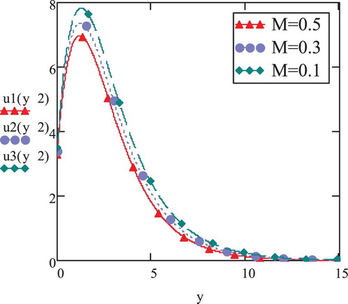
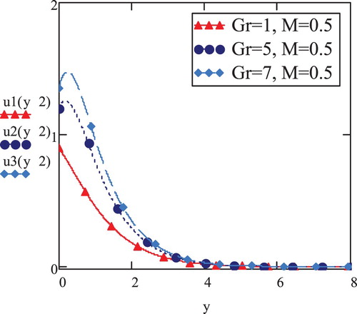
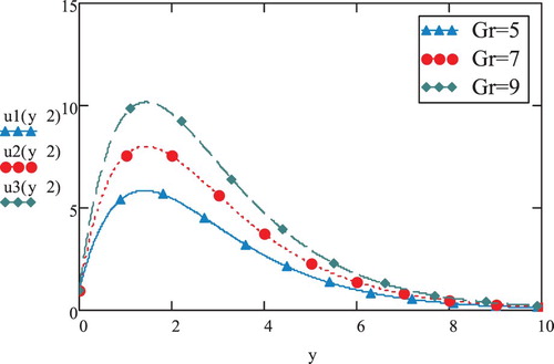
Elastoviscous fluid velocity has been plotted against varying y at t = 2 for $f\left(t\right)=1$ in Figures 2 and 3. These velocity profiles have been obtained for same magnetic field and varying values of $G_r$. The pattern of initial rise and gradual decline of velocity has been observed till it reaches its absolute minimum at higher y-values, confirming the boundary condition Equation (${13}_1$). 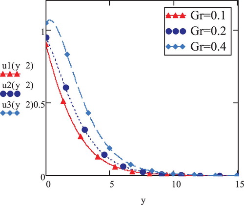An observation of sharper rise and fall of velocity magnitude corresponding to higher values of $G_r(\ge 1)$ is made in the vicinity of $0\le y\le 3$, affirming the fact that the velocity is directly related with $G_r$'s variation. However, for smaller values of $G_r(<0.5$, Figure 3), the pattern of initial increase and gradual decrease in magnitude is not retained. It rather drops continuously approaching absolute zero. Regardless of varying pattern corresponding to $G_r$-range, the decline in the magnitude of velocity, in general, for smaller values of $G_r$ is evident in both graphs. The increase in velocity due to increasing $G_r$ owes its emergence to faster movement of particles due to density differences caused by convection.

Figure 2. Viscoelastic velocity vs. y; $t=2,K=4,f\left(t\right)=1,M=0.5,\gamma =0.3,P_r=0.7,a=5$.

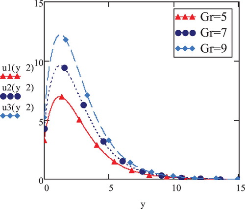
Figure 3. Viscoelastic velocity vs. y; $t=2,K=4,f\left(t\right)=1,M=0.5,\gamma =0.3,P_r=0.7,a=5$.

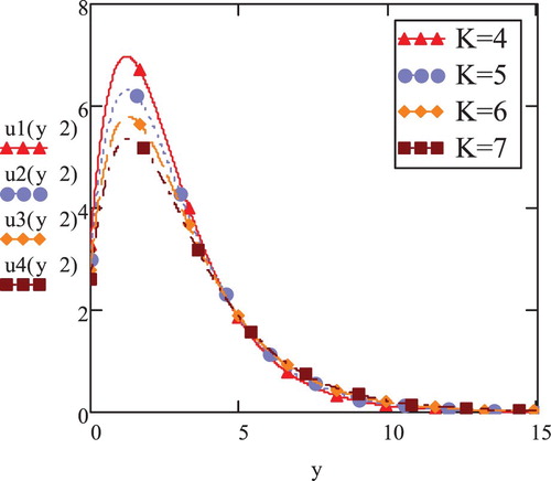
Elastoviscous parameter (K)'s influence on velocity with subsistence of magnetic field, M = 0.5 has been illustrated in Figure 4. It can be noted that velocity is inversely affected by increasing values of K. However, the profiles of velocity coincide in their decline at higher y-values. This observation complies with the fact that elastoviscous fluid, identified with higher parametric values of K endures higher resistance in its propagation, causing the magnitude of velocity to drop.

Figure 4. Viscoelastic velocity vs. y; $t=2,G_r=5,f\left(t\right)=1,M=0.5,\gamma =0.3,P_r=0.7,a=5$.

To observe the influence of magnetic field on flow propagation, Figure 5 has been obtained. Here, velocity profiles are drawn against y for varying values of Hartmann number ($f\left(t\right)=1$). In addition to following the pattern of earlier increase and then the gradual decrease in velocity, its magnitude starts decreasing for increasing magnetic field intensity and vice versa. This phenomenon shows that the presence of magnetic field of smaller magnitude can be retained to reduce the hindrance that causes the velocity of flow to drop.

Figure 5. Viscoelastic velocity vs. y; $t=2,K=4,G_r=5,f\left(t\right)=1,\gamma =0.3,P_r=0.7,a=5$.

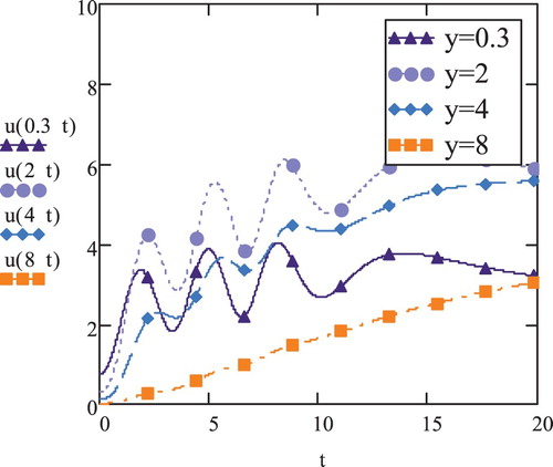
In Figures 6 and 7, we have compared the profiles of velocity of elastoviscous fluid flow against time for the cases of $\left(a\right)f\left(t\right)=1$ and $\left(b\right)f\left(t\right)=\sin \left(\omega t\right)$ (ω is frequency of oscillation) at different heights (y = 0.3, 2, 4, 8), respectively. For case (a), the velocity magnitude is slowly increasing with time along with increase in height (y = 0.3, 2). But after attaining certain height, the velocity starts dropping (y = 4, 8), corroborating that the velocity is approaching towards zero at higher y-values. It is also noted that the velocity profiles assume unchanging pattern after a certain time. For case (b), it is observed that velocity trajectories assume the pattern of oscillations along with change in time. Figure 7 also shows that the magnitude rises initially (y = 0.3, 2) but it starts dropping for higher values of $y(=4,8)$. This phenomenon is reflected in velocity profiles for y = 4 that appears below the oscillating curve for y = 2 and also for the profile of y = 8 that appears at the lowest of profiles. For higher values of y, the amplitude of oscillations begin to reduce and these oscillations are eliminated in curves for further higher values of y, turning into slowly increasing curves (y = 8). Like case (a) (Figure 6), velocity profiles for case (b) (Figure 7) remain unchanged after a certain time. Comparing the graphs for two cases, it is inspected that the velocity strength is much higher for the case (a) as compared to absolute magnitude for case (b) at corresponding y-values. Oscillating time-dependent temperature on the boundary seems to hinder the speed of flow of elastoviscous fluid.

Figure 6. Viscoelastic velocity vs. time; $f\left(t\right)=1,K=4,M=0.5,G_r=5,\gamma =0.3,P_r=0.7,a=5$.

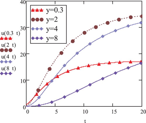
Figure 7. Viscoelastic velocity vs. time; $f\left(t\right)=\sin \left(\omega t\right),\omega =2,K=4,M=0.5,G_r=5,\gamma =0.3,P_r=0.7,a=5$.

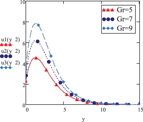
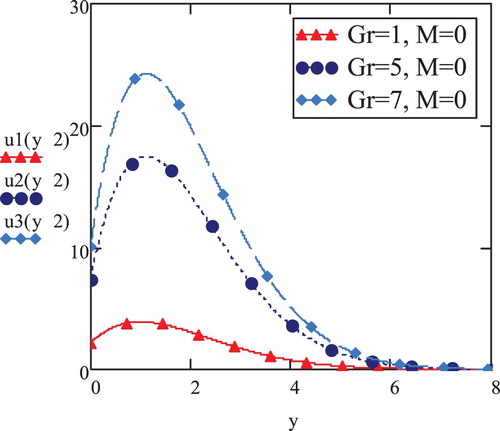
The graphs presented in Figure 8 reflect on the difference of magnitude of velocity in contrast to varying y for rising $G_r$ statistics in the disposition of $f\left(t\right)=\sin \left(\omega t\right)$. This case is compared with the scenario $f\left(t\right)=1$ (Figure 2). It is evident that in the former case ($\sin \left(\omega t\right)$), the magnitude of velocity drops for each $G_r$, however, maintaining the pattern of initial rise and decline of velocity as well as of escalation in velocity with expanding $G_r$ numbers.

Figure 8. Viscoelastic velocity vs. y; $t=2,f\left(t\right)=\sin \left(\omega t\right),\omega =2,K=4,M=0.5,G_r=5,\gamma =0.3,P_r=0.7,a=5$.

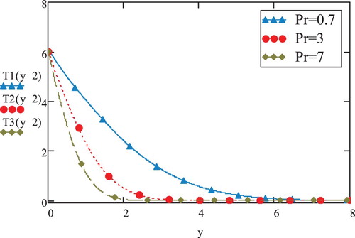
In Figure 9, the temperature variations have been conspired opposing y for different Prandtl numbers $P_r(=0.7,3,7)$ at t = 2. The temperature depreciation with enhancing Prandtl number has been observed. In general, the temperature starts dropping as y increases such that all profiles for varying $P_r$ coincide at higher y-values. The sharper decline of temperature akin to advancing Prandtl values ($P_r>1$) can be attributed to momentum transfer of flow exceeding the heat transfer flow.

Figure 9. Temperature vs. y; $t=2,\gamma =0.3,a=5$.

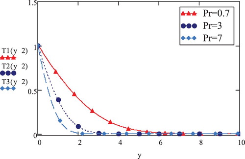
How a constant boundary condition of temperature (a = 0) influences the temperature course through fluid propagation has been discussed through Figure 10. Here, temperature profiles have been obtained against y for Prandtl number ($P_r=0.7,3,7$) as was done for the case of temporal temperature condition (Figure 9). Figure 10 displays that the constant temperature on boundary condition tends to decrease the magnitude of temperature as compared to case described by temporal temperature condition (Figure 9).

Figure 10. Temperature vs. y; $t=2,\gamma =0.3,a=0$.

To retrieve the results for Newtonian fluid propagation as well as to validate our present results, we have also obtained graphs by considering limiting values of parameters K, a and M.

Figures 11 and 12 display the velocity profiles for Newtonian fluid against y at t = 2 corresponding to rising $G_r$-values. In addition to manifestation of usual pattern of velocity increasing and then decreasing at higher y-values, velocity magnitude tends to drop in magnetic field presence (Figure 11) in comparison to the case of no magnetic field (Figure 12). Newtonian fluid velocity is also directly influenced by increasing or decreasing $G_r$, matching to elastoviscous fluid scenario. Comparing with elastoviscous fluid velocity (Figure 2), it is also validated that the velocity magnitude attains higher values for Newtonian fluid (Figure 11) due to viscous effects partaking in the elastoviscous fluid propagation.

Figure 11. Newtonian fluid velocity vs. y; $t=2,f\left(t\right)=1,\gamma =0.3,P_r=0.7,a=5$.

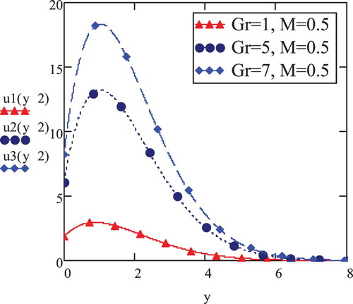
Figure 12. Newtonian fluid velocity vs. y; $t=2,f\left(t\right)=1,\gamma =0.3,P_r=0.7,a=5$.

An interesting case of Newtonian fluid's response to the condition of constant temperature on boundary has been recorded through Figure 13. These profiles show that maintaining the constant temperature on boundary tends to give a substantial drop in the velocity in comparison to temporal temperature boundary condition (Figure 11). This shows that with constant temperature on boundary, both velocity and temperature decrease.

Figure 13. Newtonian fluid velocity vs. y; $t=2,f\left(t\right)=1,\gamma =0.3,P_r=0.7,a=0$.

The case of constant velocity boundary condition ($u(0,t)=1$) for elastoviscous fluid (Figure 14) has been compared with time-dependent motion of plate with flow slip (Figure 2). It is recorded that velocity magnitude increases due to time-dependent movement of plate with fluid slipping on channel rather than the force of constant velocity brought to bear by the boundary. Evidently, the constant velocity boundary condition does not impact the direct relation of $G_r$ with elastoviscous flow velocity.

Figure 14. Viscoelastic velocity vs. y; $t=2,K=4,M=0.5,\gamma =0,P_r=0.7,a=5$.

It is interesting to note that limiting results obtained here as Equations (22(22) $\begin{array}{rl}& u(y,t)=\frac{-\left[\mathrm{\Omega }\right(P_r-1)-G_r]}{2\gamma \mathrm{\Omega }(P_r-1)\sqrt{M}}[e^{y\sqrt{M}}erfc(\frac{y}{2\sqrt{t}}+\sqrt{Mt})\\ & -e^{-y\sqrt{M}}erfc(\frac{y}{2\sqrt{t}}-\sqrt{Mt})]\\ & -\frac{\left[\mathrm{\Omega }\right(P_r-1)-G_r]}{\mathrm{\Omega }(P_r-1)(1-{\gamma }^{2}M)}erfc(\frac{y}{2\sqrt{t}}+\frac{\sqrt{t}}{\gamma })\\ & e^{-Mt+\frac{t}{{\gamma }^2}+\frac{y}{\gamma }}\\ & -\frac{G_r{e}^{\mathrm{\Omega }t}}{\mathrm{\Omega }(P_r-1)[1-{\gamma }^2(M+\mathrm{\Omega }\left)\right]}\\ & \times erfc(\frac{y}{2\sqrt{t}}+\frac{\sqrt{t}}{\gamma })e^{Mt+\frac{t}{{\gamma }^2}+\frac{y}{\gamma }}\\ & +\frac{\left[\mathrm{\Omega }\right(P_r-1)-G_r]}{2\mathrm{\Omega }(P_r-1)(1-{\gamma }^{2}M)}[e^{y\sqrt{M}}erfc(\frac{y}{2\sqrt{t}}+\sqrt{Mt})\\ & -e^{-y\sqrt{M}}erfc(\frac{y}{2\sqrt{t}}-\sqrt{Mt})]\\ & -\frac{G_r{e}^{\mathrm{\Omega }t}}{2\gamma \mathrm{\Omega }(P_r-1)\sqrt{M+\mathrm{\Omega }}}[e^{y\sqrt{M+b}}\\ & \times erfc(\frac{y}{2\sqrt{t}}+\sqrt{(M+\mathrm{\Omega })t})\\ & -e^{-y\sqrt{M+b}}erfc(\frac{y}{2\sqrt{t}}-\sqrt{(M+\mathrm{\Omega })t})]\\ & +\frac{G_r{e}^{\mathrm{\Omega }t}}{2\mathrm{\Omega }(P_r-1)[1-{\gamma }^2(M+\mathrm{\Omega }\left)\right]}\\ & \times [e^{y\sqrt{M+\mathrm{\Omega }}}erfc(\frac{y}{2\sqrt{t}}+\sqrt{(M+\mathrm{\Omega })t})+e^{-y\sqrt{M+\mathrm{\Omega }}}\end{array}$(22) )–(25(23) $\begin{array}{rl}& +\frac{G_r{e}^{\mathrm{\Omega }t}}{2\sqrt{\mathrm{\Omega }}(P_r-1)(1-{\gamma }^2\mathrm{\Omega })}\\ & \times [e^{y\sqrt{\mathrm{\Omega }}}erfc(\frac{y}{2\sqrt{t}}+\sqrt{\mathrm{\Omega }t})-e^{-y\sqrt{\mathrm{\Omega }}}\\ & \times erfc(\frac{y}{2\sqrt{t}}-\sqrt{\mathrm{\Omega }t})]\\ & +\frac{G_r\sqrt{P_r}{e}^{\mathrm{\Omega }t}}{(P_r-1)\sqrt{\mathrm{\Omega }}}{\int }_0^t\{\frac{e^{-\frac{y^2}{4s}-\mathrm{\Omega }s}}{\sqrt{\pi s}}erf\left(\sqrt{\mathrm{\Omega }(t-s)}\right)\\ & -\frac{1}{\gamma }{e}^{\frac{y}{\gamma }+\frac{s}{{\gamma }^2}-\mathrm{\Omega }s}erfc(\frac{y}{2\sqrt{s}}+\frac{\sqrt{s}}{\gamma })erf\left(\sqrt{\mathrm{\Omega }(t-s)}\right)\}\mathrm{d}s\\ & +\frac{G_{r}a}{\gamma (P_r-1)}{\int }_0^t\{\frac{e^{-\frac{y^2}{4s}}}{\sqrt{\pi s}}-\frac{1}{\gamma }{e}^{\frac{y}{\gamma }+\frac{s}{{\gamma }^2}}\\ & \times erfc(\frac{y}{2\sqrt{s}}+\frac{\sqrt{s}}{\gamma })\}{H}_3(t-s)\mathrm{d}s\\ & +\frac{G_{r}a\sqrt{P_r}}{(P_r-1)}{\int }_0^t\{\frac{e^{-\frac{y^2}{4s}}}{\sqrt{\pi s}}-\frac{1}{\gamma }{e}^{\frac{y}{\gamma }+\frac{s}{{\gamma }^2}}\end{array}$(23) ) and (28(25) $\begin{array}{rl}& u(y,t)=\frac{-\left[\mathrm{\Omega }\right(P_r-1)-G_r]}{2\gamma \mathrm{\Omega }(P_r-1)\sqrt{M}}[e^{y\sqrt{M}}erfc(\frac{y}{2\sqrt{t}}+\sqrt{Mt})\\ & -e^{-y\sqrt{M}}erfc(\frac{y}{2\sqrt{t}}-\sqrt{Mt})]\\ & -\frac{\left[\mathrm{\Omega }\right(P_r-1)-G_r]}{\mathrm{\Omega }(P_r-1)(1-{\gamma }^{2}M)}erfc(\frac{y}{2\sqrt{t}}+\frac{\sqrt{t}}{\gamma })e^{-Mt+\frac{t}{{\gamma }^2}+\frac{y}{\gamma }}\\ & -\frac{G_r{e}^{\mathrm{\Omega }t}}{\mathrm{\Omega }(P_r-1)[1-{\gamma }^2(M+\mathrm{\Omega }\left)\right]}\\ & \times erfc(\frac{y}{2\sqrt{t}}+\frac{\sqrt{t}}{\gamma })e^{Mt+\frac{t}{{\gamma }^2}+\frac{y}{\gamma }}\\ & +\frac{\left[\mathrm{\Omega }\right(P_r-1)-G_r]}{2\mathrm{\Omega }(P_r-1)(1-{\gamma }^{2}M)}[e^{y\sqrt{M}}erfc(\frac{y}{2\sqrt{t}}+\sqrt{Mt})\\ & +e^{-y\sqrt{M}}erfc(\frac{y}{2\sqrt{t}}-\sqrt{Mt})]\\ & -\frac{\left[\mathrm{\Omega }\right(P_r-1)-G_r]}{2\gamma \mathrm{\Omega }(P_r-1)\sqrt{M}}[e^{y\sqrt{M}}erfc(\frac{y}{2\sqrt{t}}+\sqrt{Mt})\\ & -e^{-y\sqrt{M}}erfc(\frac{y}{2\sqrt{t}}-\sqrt{Mt})]\\ & -\frac{G_r{e}^{\mathrm{\Omega }t}}{2\gamma \mathrm{\Omega }(P_r-1)\sqrt{M+\mathrm{\Omega }}}\\ & \times [e^{y\sqrt{M+\mathrm{\Omega }}}erfc(\frac{y}{2\sqrt{t}}+\sqrt{(M+\mathrm{\Omega })t})\\ & -e^{-y\sqrt{M+\mathrm{\Omega }}}erfc(\frac{y}{2\sqrt{t}}-\sqrt{(M+\mathrm{\Omega })t})]\\ & +\frac{G_r{e}^{\mathrm{\Omega }t}}{2\mathrm{\Omega }(P_r-1)[1-{\gamma }^2(M+\mathrm{\Omega }\left)\right]}\end{array}$(25) ) are seen to be matching previously obtained results [18,25] for $G_m\to 0$ & $F\to 0$, hence validating the exactitude of our current method and outcomes.

6. Conclusion

We have determined the exact expressions of velocity and temperature of elastoviscous MHD fluid slipping past an unbounded upright plate with vacillating temperature. These expressions are obtained for a free convection flow. The main results have been collected as follows:

1. Elastoviscous fluid velocity was discussed for constant temperature, $f\left(t\right)=1$, and variable temperature, $f\left(t\right)=\sin \left(\omega t\right)$, on the boundary. It was established that at a proposed time and magnetic field, initial rise in the velocity is ascertained that gives way to abating magnitude ($G_r\ge 1$) for advancing y values. However, for smaller values of $G_r$, owing to empowering viscous forces, the velocity continues to decrease unlike the pattern of initial rise and the drop for $G_r\ge 1$. An observation of drop in the magnitude of elastoviscous velocity was also made for variable temperature case. The constant temperature on boundary tends to play its role in accelerating the motion of particles of fluid, causing the velocity to rise.

2. In magnetic habitation, elastoviscous fluid velocity tends to be inversely proportional to elastoviscous parameter, K. Here, the velocity deteriorates for higher values of K in accordance with phenomenon of escalation of viscous forces in this case and vice versa.

3. Elastoviscous fluid velocity is directly influenced by values of $G_r$, Grashof (thermal) number, and is inversely affected by M, Hartmann number. The higher value of $G_r$ plays its role in raising the conduction strength that overcomes the resistance caused by viscous forces, hence increasing the velocity of fluid.

4. Elastoviscous fluid velocity against time displays the slowly increasing profiles (it retains the pattern of unchanging trajectories after a certain time) for constant temperature on the boundary and oscillating pattern velocity profiles for variable temperature ($f\left(t\right)=\sin \left(\omega t\right)$). Oscillations in the later case start ebbing away after a certain time, turning the profiles into slowly rising curves. Also, the hindrance to flow caused by oscillating variable temperature is observed in terms of drop in the magnitude of velocity.

5. Temperature decrease due to increasing Prandtl number, $P_r$, has been recorded both for variable temperature and constant temperature administered on extremity of flat upstanding channel.

6. The results of Newtonian fluid velocity corresponding to the cases of absence of magnetic field, constant temperature and uniform velocity allowed at the end on channel were retrieved and validated to be accurate. Analogous to elastoviscous fluid scenario, Newtonian fluid velocity increments due to inflating $G_r$ numbers and vice versa. Also, in magnetic occupation, the velocity drops as to the situation of non-existent magnetic field. Due to lesser viscous effects, Newtonian fluid velocity's magnitude is validated to be higher than elastoviscous velocity.

7. Non-varying temperature boundary condition tends to bring on a considerable drop in the magnitude of velocity of velocity of Newtonian fluid, opposite to elastoviscous case.

8. An interesting phenomenon of developing elastoviscous velocity corresponding to time-dependent motion of plate with flow slip was also observed unlike the non-varying velocity on extremity of plate. However, the variation of boundary condition of velocity does not affect the direct relation of velocity with thermal Grashof number, $G_r$.

Nomenclature

$u(y,t)$	=	velocity (m/s)
$T(y,t)$	=	temperature (K)
ρ	=	density of fluid (kg/m${}^3$)
ν	=	kinematic viscosity (m${}^2$/s)
σ	=	electrical conductivity (S/m)
κ	=	thermal conductivity (J/(s·m·K))
$C_p$	=	specific heat at constant pressure (J/(kg·K))
$q_r$	=	radiation heat flux (J/(s·m${}^2$))
β	=	thermal expansion coefficient (1/K)
g	=	gravitational acceleration (m/s${}^2$)
M	=	Hartmann number (dimensionless)
$G_r$	=	thermal Grashof number (dimensionless)
F	=	thermal radiation parameter (J/(s·m${}^2$))
$P_r$	=	Prandtl number (dimensionless)
ω	=	frequency of oscillation (1/s)

Disclosure statement

No potential conflict of interest was reported by the authors.

ORCID

Cemil Tunç  http://orcid.org/0000-0003-2909-8753

Appendix

(A1) $\begin{array}{rl}& \frac{1}{(s-\lambda {)}^2-(\sqrt{\tau }{)}^2}=\frac{1}{2\sqrt{\tau }}\frac{1}{s-(\lambda +\sqrt{\tau })}-\frac{1}{2\sqrt{\tau }}\frac{1}{s-(\lambda -\sqrt{\tau })},\end{array}$(A1) (A2) $\begin{array}{rl}& \frac{1}{s\left[\right(s-\lambda {)}^2-\left(\sqrt{\tau }{)}^2\right]}=\frac{1}{({\lambda }^2-\tau )}\frac{1}{s}+\frac{1}{(2\lambda \sqrt{\tau }+2\tau )}\\ & \times \frac{1}{s-(\lambda +\sqrt{\tau })}+\frac{1}{(2\tau -2\lambda \sqrt{\tau })}\frac{1}{s-(\lambda -\sqrt{\tau })},\end{array}$(A2) (A3) $\begin{array}{rl}& {\mathcal{L}}^{-1}\{\frac{e^{-p\sqrt{s}}}{\sqrt{s}+b}\}=\frac{e^{-\frac{p^2}{4t}}}{\sqrt{\pi t}}-b{e}^{pb+b^{2}t}erfc(\frac{p}{2p\sqrt{t}}+b\sqrt{t}),\end{array}$(A3) (A4) $\begin{array}{rl}& {\mathcal{L}}^{-1}\{e^{\frac{p}{s}}-1\}=\sqrt{\frac{p}{t}}{I}_1\left(2\sqrt{pt}\right),\end{array}$(A4) (A5) $\begin{array}{rl}& {\mathcal{L}}^{-1}\{e^{-p\sqrt{s}}\}=\frac{p}{2\sqrt{\pi t^3}}{e}^{-\frac{p^2}{4t}},\end{array}$(A5) (A6) $\begin{array}{rl}& {\mathcal{L}}^{-1}\{\frac{e^{-p\sqrt{s}}}{s}\}=erfc(\frac{p}{2\sqrt{t}}),\end{array}$(A6) (A7) $\begin{array}{rl}& {\mathcal{L}}^{-1}\{\frac{\sqrt{s}}{s-p^2}\}=\frac{1}{\sqrt{\pi t}}+p{e}^{p^{2}t}erf\left(p\sqrt{t}\right),\end{array}$(A7) (A8) $\begin{array}{rl}& {\mathcal{L}}^{-1}\{\frac{1}{\sqrt{s}(s-p^2)}\}=\frac{1}{p}{e}^{p^{2}t}erf\left(p\sqrt{t}\right),\end{array}$(A8) (A9) $\begin{array}{rl}& \frac{2iu}{\sqrt{\pi }}{\int }_0^t{s}^{-\frac{1}{2}}{e}^{u^{2}s-\frac{a^2}{4s}}\mathrm{d}s=[e^{-2iu\frac{a}{2}}erfc(\frac{a}{2\sqrt{t}}-iu\sqrt{t})\\ & -e^{2iu\frac{a}{2}}erfc(\frac{a}{2\sqrt{t}}+iu\sqrt{t})],\end{array}$(A9) (A10) $\begin{array}{rl}& \frac{2a}{\sqrt{\pi }}{\int }_0^t{s}^{-\frac{3}{2}}{e}^{u^{2}s-\frac{a^2}{4s}}\mathrm{d}s=[e^{-2iu\frac{a}{2}}erfc(\frac{a}{2\sqrt{t}}-iu\sqrt{t})\\ & +e^{2iu\frac{a}{2}}erfc(\frac{a}{2\sqrt{t}}+iu\sqrt{t})].\end{array}$(A10)

References

- Hossain MA, Takhar HS. Radiation effect on mixed convection along a vertical plate with uniform surface temperature. Heat Mass Transf. 1996;31(4):243–248.
- Vajravelu K, Hadjiricaloou A. Convective heat transfer in an electrically conducting fluid at a stretching surface with uniform free stream. Int J Eng Sci. 1997;35:1237–1244.
- Forsberg CW. Hydrogen, nuclear energy and the advanced high-temperature reactor. Int J Hydrog Energy. 2003;28(10):1073–1081.
- Yildiz B, Kazimi MS. Efficiency of hydrogen production systems using alternative nuclear energy technologies. Int J Hydrog Energy. 2006;31(1):77–92.
- Soundalgekar VM, Warve PD. Unsteady free convection flow past an infinite vertical plate with mass transfer. Int J Heat Mass Transf. 1977;20:1363–1373.
- Soundalgekar VM. Free convection effects on the flow past a vertical oscillating plate. Astrophys Space Sci. 1979;60:165–172.
- Mazumdar MK, Deka RK. MHD flow past an impulsively started infinite vertical plate in presence of thermal radiation. Rom J Phys. 2007;52(5-6):529–535.
- Deka RK, Neog BC. Combined effects of thermal radiation and chemical reaction on free convection flow past a vertical plate in porous medium. Adv Appl Fluid Mech. 2009;6:181–195.
- Khaleque ST, Samad MA. Effects of radiation, heat generation and viscous dissipation on MHD free convection flow along a stretching sheet. Res J Appl Sci Eng Tech. 2010;2(4):368–377.
- Singh AK. Mass transfer effects on the flow past an accelerated vertical plate with constant heat flux. Astrophys Space Sci. 1983;97(1):57–61.
- Singh AK. Oscillatory free-convective flow of an elastico-viscous fluid past an impulsively started infinite vertical porous plate, II. Astrophys Space Sci. 1984;105(2):307–313.
- Singh AK, Singh AK, Singh NP. Heat and mass transfer in MHD flow of a viscous fluid past a vertical plate under oscillatory suction velocity. Indian J Pure Appl Math. 2003;34:429–433.
- Chen CH. Combined heat and mass transfer in MHD free convection from a vertical surface with ohmic heating and viscous dissipation. Int J Eng Sci. 2004;42:699–713.
- Acharya M, Dash GC, Singh LP. Effect of chemical and thermal diffusion with Hall current on unsteady hydromagnetic flow near an infinite vertical porous plate. J Phys D Appl Phys. 1995;28:2455–2464.
- Acharya M, Dash GC, Singh LP. Hall effect with simultaneous thermal and mass diffusion on unsteady hydromagnetic flow near an accelerated vertical plate. Indian J Phys. 2001;75B:68–70.
- Aboeldahab EM, Elbarbary EME. Hall current effect magneto-hydrodynamics free convection flow past a semi.-infinite vertical plate with mass transfer. Int J Eng Sci. 2001;39:1641–1652.
- Vieru D, Fetecau C, Sohail A. Flow due to a plate that applies an accelerated shear to a second grade fluid between two parallel walls perpendicular to the plate. Z Angew Math Phys. 2011;62:161–172.
- Fetecau C, Vieru D, Fetecau C. Effect of side walls on the motion of a viscous fluid induced by an infinite plate that applies an oscillating shear stress to the fluid. Cent Eur J Phys. 2011;9(3):816–824.
- Liu Y, Zheng L. Unsteady MHD Couette flow of a generalized Oldroyd-B fluid with fractional derivative. Comput Math Appl. 2011;61:443–450.
- Zheng L, Liu Y, Zhang X. Exact solutions for MHD ow of generalized Oldroyd-B fluid MHD ow of generalized Oldroyd-B fluid due to an infinite accelerating plate. Math Comput Model. 2011;54(1-2):780–788.
- Zheng L, Wang KN, Gao YT. Unsteady ow and heat transfer of a generalized Maxwell fluid due to a hyperbolic sine accelerating plate. Comput Math Appl. 2011;61(8):2209–2212.
- Zheng L, Liu Y, Zhang X. Slip effects on MHD ow of a generalized Oldroyd-B fluid with fractional derivative. Non-linear Anal-Real. 2012;13(2):513–523.
- Rana M, Shahid N, Ali Zafar A. Effects of side walls on the motion induced by an infinite plate that applies shear stresses to an Oldroyd-B fluid. Z Naturforsch A. 2014;68(12):725–734.
- Waqas H, Khan SU, Hassan M, et al. Analysis on the bioconvection flow of modified second-grade nanofluid containing gyrotactic microorganisms and nanoparticles. J Mol Liq. 2019;219:111231.
- Shahid N. An analytical study of adversely affecting radiation and temperature parameters on a magnetohydrodynamic elasto-viscous fluid. Math Comput Appl. 2019;24(1):31.
- Huang C, Zhang Y. Calculation of high-temperature insulation parameters and heat transfer behaviours of multilayer insulation by inverse problems method. Chinese J Aeronaut. 2014;27(4):791–796.
- Zhang C, Zheng L, Zhang X, et al. MHD flow and radiation heat transfer of nano fluids in porous media with variable surface heat flux and chemical reaction. Appl Math Model. 2015;39(1):165–181.
- Tripathi D, Gupta PK, Das S. Influence of slip condition on peristaltic transport of a viscoelastic fluid with model. Therm Sci. 2011;15:501–515.
- Jamil M, Rauf A, Zafar AA, et al. New exact analytical solutions for Stokes' first problem of Maxwell fluid with fractional derivative approach. Comput Math Appl. 2011;62:1013–1023.
- Jamil M, Khan NA, Shahid N. Fractional MHD Oldroyd-B fluid over an oscillating plate. Therm Sci. 2013;17(4):997–1011.
- Shahid N. A study of heat and mass transfer in a fractional MHD flow over an infinite oscillating plate. SpringerPlus. 2015;4:1. doi:10.1186/s40064-015-1426-4.
- Shahid N. Effects of thermal radiation and mass diffusion on MHD flow over a vertical plate applying time-dependent shear to the fluid. Neural Parallel Sci Comput. 2016;24(4):431–452.
- Ellahi R. The effects of MHD and temperature dependent viscosity on the flow of non-Newtonian nanofluid in a pipe: analytical solutions. Appl Math Model. 2019;37(3):1451–1457.
- Shehzad N, Zeeshan A, Ellahi R. Electroosmotic flow of MHD power law Al2O3-PVC nanofluid in a horizontal channel: Couette-Poiseuille flow model. Commun Theor Phys. 2018;69(6):655–666.
- Ellahi R, Alamri SZ, Basit A, et al. Effects of MHD and slip on heat transfer boundary layer flow over a moving plate based on specific entropy generation. J Taibah Univ Sci. 2018;12(4):476–482.
- Ellahi R, Zeeshan A, Shehzad N, et al. Structural impact of Kerosene-Al2O3 nanoliquid on MHD Poiseuille flow with variable thermal conductivity: application of cooling process. J Mol Liq. 2018;264:607–615.
- Ellahi R, Sait SM, Shehzad N, et al. Numerical simulation and mathematical modeling of electroosmotic Couette-Poiseuille flow of MHD power-law nanofluid with entropy generation. Symmetry. 2019;11(8):1038.
- Ellahi R, Zeeshan A, Hussain F, et al. Thermally charged MHD bi-phase flow coatings with non-Newtonian nanofluid and Hafnium particles through slippery walls. Coatings. 2019;9(5):300.
- Thoi TN, Bhatti MM, Ali JA, et al. Analysis on the heat storage unit through a Y-shaped fin for solidification of NEPCM. J Mol Liq. 2019;292:111378.
- Zeeshan A, Abbas T, Ellahi R. Effects of radiative electro-magnetohydrodynamics diminishing internal energy of pressure-driven flow of titanium dioxide-water nanofluid due to entropy generation. Entropy. 2019;21(236):1–25.
- Yousif MA, Ismael HF, Abbas T, et al. Numerical study of momentum and heat transfer of MHD Carreau nanofluid over exponentially stretched plate with internal heat source/sink and radiation. Heat Transf Res. 2019;50(7):649–658.
- Landau LD, Llfshltz EM. Fluid mechanics. New York, NY: Elsevier; 1978.