An efficient numerical technique for a new fractional tuberculosis model with nonsingular derivative operator

Abstract

The present study aims to investigate a new fractional model describing the dynamical behaviour of the tuberculosis infection. In this new formulation, we use a recently introduced fractional operator with Mittag–Leffler nonsingular kernel. To solve and simulate the proposed model, a new and efficient numerical method is developed based on the product-integration rule. Simulation results are provided and some discussions are given to verify the theoretical analysis. The results indicate that employing the nonsingular operator can extract the hidden aspects of the model under consideration while these features are invisible when we use the ordinary time-derivatives. Therefore, the non-integer calculus supplies more flexible models describing the asymptotic behaviours of the real-world phenomena and helps us to better understand their complex dynamics.

Keywords:

• Tuberculosis disease
• fractional model
• nonsingular kernel
• numerical method
• nonlocal dynamics

1. Introduction

Mathematical modelling is an important tool to describe different aspects of the natural phenomena more precisely. Among the existing excellent works in this direction, the mathematical models for different kinds of diseases have extensively attracted the attention of many scientists. One of the main advantages in this area is to identify the impressive factors preventing the spread of diseases for the purpose of treatment. This property makes this field of study more attractive for both mathematicians and biologists. Recently, the fractional calculus has been widely used to model and describe the biological processes. Some noticeable efforts have been done in [1–3] for the fractional modelling of membrane charging, nerve axon and vestibular ocular models, viscoelastic model of cells, etc. In recent years, the non-integer calculus has also been employed to investigate and discuss the spread of diseases. In [4], the malaria transmission was modelled by a fractional formalism. In [5], a time-fractional model of immunogenic tumour was studied. In [6], a fractional model of HIV infection was introduced. In [7], a fractional HIV/HCV coinfection model was employed for the effect of HIV viral load. More recent study in this direction can also be found in [8].

Tuberculosis is a bacterial disease, which is known as one of the most important causes of death in the world [9]. This disease is caused by Mycobacterium tuberculosis and spread with active tuberculosis through the air by people. A good review on the mathematical model of tuberculosis can be found in [10]. In [11], an interesting model was investigated for this infectious disease for the purpose of treatment by an optimal control strategy. In [12], a time-delay model was introduced for the tuberculosis. In [13], numerical simulations were provided using the tuberculosis data from Angola. In [14], a new tuberculosis model was developed to investigate the impact of treatment for both latently and actively infected tuberculosis populations. In [15], a tuberculosis dynamic was studied and used to reduce the infection in the Philippines' population. As well as numerous works mentioned above, there are some studies on the fractional modelling of tuberculosis infection. In [16], a fractional multi-strain tuberculosis model was proposed and an approximation technique was developed to obtain the endemic solution. In [17], a fractional analysis was carried out to identify the transmission dynamic of a tuberculosis model. In [18], a new fractional model was introduced for the tuberculosis infection. In [19], the authors developed a fractional model to explore the impact of diabetes and resistant strains on the dynamic of tuberculosis. In [20], the tuberculosis dynamic was explored by a fractional-order model in the Caputo sense. In [21], an optimal control strategy was studied for a fractional tuberculosis model containing the effect of diabetes and resistant strains.

In recent years, the fractional calculus has gained the importance and popularity for the modelling of the real-world problems [22–28]. However, many scientists have shown that the conventional form of the fractional derivatives with singular kernel may not be able to characterize the nonlocal dynamics in an appropriate manner; hence, to better investigate the real-world phenomena with hereditary property, there is a need to apply new types of the fractional operators with nonsingular kernel. For this purpose, a new differential operator with Mittag–Leffler (ML) kernel (ABC) has been recently developed in [29] and its main properties have been deeply investigated [30, 31]. Nowadays, this new operator has been extensively applied to describe many realistic systems [32–35]; however, the application of this operator for more practical cases (such as those in [36, 37]) should be explored and extended. In addition, more efficient numerical methods need to be improved to solve the ABC fractional models effectively. This motivates us to study the characteristics of the tuberculosis infection by using its new formulation in the fractional ABC calculus. We also develop an efficient numerical technique on the basis of the product-integration (PI) rule to solve the above-mentioned equations properly. Simulation results indicate that employing nonsingular operator can extract the hidden aspects of the model under consideration, which may be invisible when we use this model in a classic integer manner. Therefore, more flexible models are available by the non-integer calculus to investigate the real-world phenomena and understand their complex dynamics.

The rest of this paper is organized as follows. Some preliminary results are given in Section 2. Section 3 is devoted to the new fractional tuberculosis model and its main characteristics. A generalized numerical method is proposed in Section 4 solving the ABC tuberculosis model. Numerical and comparative are provided in Section 5. Finally, the paper is finished in Section 6 by some concluding remarks.

2. Preliminary results

In this section, some preliminaries are presented for the new direction of the non-integer calculus involving the nonsingular operators. Following [29], we introduce the ABC operator with ML kernel and recall its main characteristics.

Definition 2.1

Let 0<t<T and $\phi \in {\mathbb{H}}^1(0,T)$. Then, the ABC fractional operator of order $\zeta \in (0,1)$ of the function φ is given by (1) $\begin{array}{r}{}_0^{ABC}{D}_t^{\zeta }\phi \left(t\right)=\frac{A\left(\zeta \right)}{1-\zeta }{\int }_0^t{E}_{\zeta }\left[-\theta (t-\rho {)}^{\zeta }\right]\frac{\mathrm{d}\phi \left(\rho \right)}{\mathrm{d}\rho }\mathrm{d}\rho ,\end{array}$(1) where $\theta =\zeta /\left(1-\zeta \right)$, $A\left(\zeta \right)$ with the property $A\left(0\right)=A\left(1\right)=1$ denotes the normalization function, and $E_{\zeta }$ is the one-parameter ML function. The associated integral operator is also given as (2) $\begin{array}{rl}{}_0^{ABC}{I}_t^{\zeta }\phi \left(t\right)& =\frac{1-\zeta }{A\left(\zeta \right)}\phi \left(t\right)\\ & +\frac{\zeta }{A\left(\zeta \right)\mathrm{\Gamma }\left(\zeta \right)}{\int }_0^t(t-\rho {)}^{\zeta -1}\phi (\rho )\mathrm{d}\rho .\end{array}$(2)

Note that, the integral operator (2(2) $\begin{array}{rl}{}_0^{ABC}{I}_t^{\zeta }\phi \left(t\right)& =\frac{1-\zeta }{A\left(\zeta \right)}\phi \left(t\right)\\ & +\frac{\zeta }{A\left(\zeta \right)\mathrm{\Gamma }\left(\zeta \right)}{\int }_0^t(t-\rho {)}^{\zeta -1}\phi (\rho )\mathrm{d}\rho .\end{array}$(2) ) recovers the original function when $\zeta =0$, while it becomes the ordinary integral for $\zeta =1$.

Definition 2.2

The constant ${\phi }^{\ast }$ is the equilibrium point of the system ${}_0^{ABC}{D}_t^{\zeta }\varphi \left(t\right)=f\left(\phi \right(t\left)\right)$ with the initial condition $\phi \left(0\right)={\phi }_0$ if and only if $f\left({\phi }^{\ast }\right)=0$.

In the following, some useful properties are given for the ABC fractional operator [29].

Property 2.1

Let ${\phi }_1,{\phi }_2\in {\mathbb{H}}^1(0,T)$ be such that ${}_0^{ABC}{D}_t^{\zeta }{\phi }_1\left(t\right),{}_0^{ABC}{D}_t^{\zeta }{\phi }_2\left(t\right)$ exist a.e., and $k_1,k_2\in \mathbb{R}$. Then, the expression ${}_0^{ABC}{D}_t^{\zeta }\left(k_1{\phi }_1\right(t)+k_2{\phi }_2(t\left)\right)$ exists a.e., and (3) $\begin{array}{rl}& {}_0^{ABC}{D}_t^{\zeta }\left(k_1{\phi }_1\right(t)+k_2{\phi }_2(t\left)\right)\\ & =k_1{}_0^{ABC}{D}_t^{\zeta }{\phi }_1\left(t\right)+k_2{}_0^{ABC}{D}_t^{\zeta }{\phi }_2\left(t\right).\end{array}$(3)

Property 2.2

For a constant function $\phi \left(t\right)\equiv c$, the ABC operator is zero, i.e. (4) ${}_0^{ABC}{D}_t^{\zeta }c=0.$(4)

Property 2.3

The Laplace transform of the ABC differential operator is in the form (5) $\mathfrak{L}\left\{{}_0^{ABC}{D}_t^{\zeta }\phi \left(t\right)\right\}\left(p\right)=\frac{A\left(\zeta \right)}{1-\zeta }\frac{p^{\zeta }\mathfrak{L}\left\{\phi \left(t\right)\right\}\left(p\right)}{p^{\zeta }+\frac{\zeta }{1-\zeta }}.$(5)

Property 2.4

The following useful relation is satisfied between the operators (1(1) $\begin{array}{r}{}_0^{ABC}{D}_t^{\zeta }\phi \left(t\right)=\frac{A\left(\zeta \right)}{1-\zeta }{\int }_0^t{E}_{\zeta }\left[-\theta (t-\rho {)}^{\zeta }\right]\frac{\mathrm{d}\phi \left(\rho \right)}{\mathrm{d}\rho }\mathrm{d}\rho ,\end{array}$(1) ) and (2(2) $\begin{array}{rl}{}_0^{ABC}{I}_t^{\zeta }\phi \left(t\right)& =\frac{1-\zeta }{A\left(\zeta \right)}\phi \left(t\right)\\ & +\frac{\zeta }{A\left(\zeta \right)\mathrm{\Gamma }\left(\zeta \right)}{\int }_0^t(t-\rho {)}^{\zeta -1}\phi (\rho )\mathrm{d}\rho .\end{array}$(2) ) (6) ${}_0^{ABC}{I}_t^{\zeta }\left[{}_0^{ABC}{D}_t^{\zeta }\phi \left(t\right)\right]=\phi \left(t\right)-\phi \left(0\right).$(6)

Property 2.5

For each $\phi \in {\mathbb{H}}^1(0,T)$, the operator (1(1) $\begin{array}{r}{}_0^{ABC}{D}_t^{\zeta }\phi \left(t\right)=\frac{A\left(\zeta \right)}{1-\zeta }{\int }_0^t{E}_{\zeta }\left[-\theta (t-\rho {)}^{\zeta }\right]\frac{\mathrm{d}\phi \left(\rho \right)}{\mathrm{d}\rho }\mathrm{d}\rho ,\end{array}$(1) ) satisfies (7) $∥{}_0^{ABC}{D}_t^{\zeta }\phi \left(t\right)∥\le \frac{A\left(\zeta \right)}{1-\zeta }∥\phi \left(t\right)∥,$(7) where $\parallel \phi \left(t\right)\parallel =\underset{0\le t\le T}{max}|\phi \left(t\right)|$.

Property 2.6

The ABC operator (1(1) $\begin{array}{r}{}_0^{ABC}{D}_t^{\zeta }\phi \left(t\right)=\frac{A\left(\zeta \right)}{1-\zeta }{\int }_0^t{E}_{\zeta }\left[-\theta (t-\rho {)}^{\zeta }\right]\frac{\mathrm{d}\phi \left(\rho \right)}{\mathrm{d}\rho }\mathrm{d}\rho ,\end{array}$(1) ) fulfils the Lipschitz condition, i.e. for each ${\phi }_1,{\phi }_2\in {\mathbb{H}}^1(0,T)$ there exists a constant L>0 such that (8) $∥{}_0^{ABC}{D}_t^{\zeta }{\phi }_1\left(t\right)-{}_0^{ABC}{D}_t^{\zeta }{\phi }_2\left(t\right)∥\le L∥{\phi }_1\left(t\right)-{\phi }_2\left(t\right)∥.$(8)

Some additional information is available in [29, 38], which the interested readers can refer to.

3. The new fractional tuberculosis model

This section develops a new fractional version of a tuberculosis model in the ABC sense with incomplete treatment. The original version of this model including integer-order derivatives has been previously examined in [39]; however, the influence of hereditary, as a fundamental feature of many biological processes, has not been included in this model. To overcome this drawback, we employ the newly introduced ABC operator (1(1) $\begin{array}{r}{}_0^{ABC}{D}_t^{\zeta }\phi \left(t\right)=\frac{A\left(\zeta \right)}{1-\zeta }{\int }_0^t{E}_{\zeta }\left[-\theta (t-\rho {)}^{\zeta }\right]\frac{\mathrm{d}\phi \left(\rho \right)}{\mathrm{d}\rho }\mathrm{d}\rho ,\end{array}$(1) ) instead of ordinary time-derivative in the tuberculosis model since the ABC operator essentially includes the effect of memory in its definition. In addition, according to [40], we modify the fractional operator by an auxiliary parameter σ, having the dimension of sec., to ensure that the right- and left-hand sides of the resultant equation possess the same dimension $s^{-1}$. Considering these features, the new transmission model of the tuberculosis infection takes the form (9) $\begin{array}{rl}\frac{1}{{\sigma }^{1-\zeta }}{}_0^{ABC}{D}_t^{\zeta }S\left(t\right)& =\mathrm{\Lambda }-\mu S\left(t\right)-bS\left(t\right)I\left(t\right),t\ge 0,\\ \frac{1}{{\sigma }^{1-\zeta }}{}_0^{ABC}{D}_t^{\zeta }L\left(t\right)& =-(\mu +\epsilon )L\left(t\right)+(1-k)\delta T\left(t\right)\\ & +bI\left(t\right)S\left(t\right),t\ge 0,\\ \frac{1}{{\sigma }^{1-\zeta }}{}_0^{ABC}{D}_t^{\zeta }I\left(t\right)& =-(\mu +\gamma +a_1)I\left(t\right)+k\delta T\left(t\right)\\ & +\epsilon L\left(t\right),t\ge 0,\\ \frac{1}{{\sigma }^{1-\zeta }}{}_0^{ABC}{D}_t^{\zeta }T\left(t\right)& =-(\mu +\delta +a_2)T\left(t\right)+\gamma I\left(t\right),t\ge 0,\end{array}$(9) along with the initial conditions (10) $S\left(0\right)=S_0,L\left(0\right)=L_0,I\left(0\right)=I_0,T\left(0\right)=T_0.$(10) As can bee seen, the fractional operator in Equation (9(9) $\begin{array}{rl}\frac{1}{{\sigma }^{1-\zeta }}{}_0^{ABC}{D}_t^{\zeta }S\left(t\right)& =\mathrm{\Lambda }-\mu S\left(t\right)-bS\left(t\right)I\left(t\right),t\ge 0,\\ \frac{1}{{\sigma }^{1-\zeta }}{}_0^{ABC}{D}_t^{\zeta }L\left(t\right)& =-(\mu +\epsilon )L\left(t\right)+(1-k)\delta T\left(t\right)\\ & +bI\left(t\right)S\left(t\right),t\ge 0,\\ \frac{1}{{\sigma }^{1-\zeta }}{}_0^{ABC}{D}_t^{\zeta }I\left(t\right)& =-(\mu +\gamma +a_1)I\left(t\right)+k\delta T\left(t\right)\\ & +\epsilon L\left(t\right),t\ge 0,\\ \frac{1}{{\sigma }^{1-\zeta }}{}_0^{ABC}{D}_t^{\zeta }T\left(t\right)& =-(\mu +\delta +a_2)T\left(t\right)+\gamma I\left(t\right),t\ge 0,\end{array}$(9) ) has been taken in the sense of ABC with $\zeta \in (0,1)$. A physical description of the parameters and variables is given as below. The total population is partitioned into four distinct categories depending on their epidemiological stages. The first category, which is denoted by $S\left(t\right)$, includes the susceptible individuals. This population is never infected by the tuberculosis. The second compartment is denoted by $L\left(t\right)$ and contains the latent infected persons. Although these people have been infected, they do not have the symptoms of the disease, and they are not infectious as well. The next compartment is the population of infectious individuals, which is signified by $I\left(t\right)$, has active tuberculosis, can transmit the infection, and is not in treatment. The last group, denoted by $R\left(t\right)$, is the population of infected individuals, which is under treatment. Since the state variables in (9(9) $\begin{array}{rl}\frac{1}{{\sigma }^{1-\zeta }}{}_0^{ABC}{D}_t^{\zeta }S\left(t\right)& =\mathrm{\Lambda }-\mu S\left(t\right)-bS\left(t\right)I\left(t\right),t\ge 0,\\ \frac{1}{{\sigma }^{1-\zeta }}{}_0^{ABC}{D}_t^{\zeta }L\left(t\right)& =-(\mu +\epsilon )L\left(t\right)+(1-k)\delta T\left(t\right)\\ & +bI\left(t\right)S\left(t\right),t\ge 0,\\ \frac{1}{{\sigma }^{1-\zeta }}{}_0^{ABC}{D}_t^{\zeta }I\left(t\right)& =-(\mu +\gamma +a_1)I\left(t\right)+k\delta T\left(t\right)\\ & +\epsilon L\left(t\right),t\ge 0,\\ \frac{1}{{\sigma }^{1-\zeta }}{}_0^{ABC}{D}_t^{\zeta }T\left(t\right)& =-(\mu +\delta +a_2)T\left(t\right)+\gamma I\left(t\right),t\ge 0,\end{array}$(9) ) reflect the human population, they are all assumed to be non-negative. From the first equation in (9(9) $\begin{array}{rl}\frac{1}{{\sigma }^{1-\zeta }}{}_0^{ABC}{D}_t^{\zeta }S\left(t\right)& =\mathrm{\Lambda }-\mu S\left(t\right)-bS\left(t\right)I\left(t\right),t\ge 0,\\ \frac{1}{{\sigma }^{1-\zeta }}{}_0^{ABC}{D}_t^{\zeta }L\left(t\right)& =-(\mu +\epsilon )L\left(t\right)+(1-k)\delta T\left(t\right)\\ & +bI\left(t\right)S\left(t\right),t\ge 0,\\ \frac{1}{{\sigma }^{1-\zeta }}{}_0^{ABC}{D}_t^{\zeta }I\left(t\right)& =-(\mu +\gamma +a_1)I\left(t\right)+k\delta T\left(t\right)\\ & +\epsilon L\left(t\right),t\ge 0,\\ \frac{1}{{\sigma }^{1-\zeta }}{}_0^{ABC}{D}_t^{\zeta }T\left(t\right)& =-(\mu +\delta +a_2)T\left(t\right)+\gamma I\left(t\right),t\ge 0,\end{array}$(9) ), the recruitment of individuals can increase the susceptible population at a rate Λ. The coefficient μ is the natural death rate of all individuals. The contact between susceptible and infectious individuals acquire the tuberculosis infection within a transmission coefficient b. After being infected, the individual first enters the latently infected population at a rate $bI\left(t\right)S\left(t\right)$, and then becomes infectious at a rate ϵ. By detecting an infectious individual, he/she will be treated and enter the treatment compartment. The parameter γ is the per-capita treatment rate of infected population. At a rate δ, a treated individual leaves his/her population. However, the treatment may fail and the treated person may enter the compartment I; otherwise, due to the remainder of Mycobacterium tuberculosis, the treated individual becomes latently infectious and enters the population L. The failure of the treatment is reflected by the parameter k ($0\le k\le 1$), where k = 1 denotes the complete failure of the treatment, i.e. all the treated individuals are still infectious, while k = 0 expresses that all the treated persons have become latently infectious. The parameters $a_1$ and $a_2$ also denote the tuberculosis-induced death rate of the infectious and under treatment individuals, respectively.

3.1. Non-negative solution

In this section, we show that the feasibility region of the system (9(9) $\begin{array}{rl}\frac{1}{{\sigma }^{1-\zeta }}{}_0^{ABC}{D}_t^{\zeta }S\left(t\right)& =\mathrm{\Lambda }-\mu S\left(t\right)-bS\left(t\right)I\left(t\right),t\ge 0,\\ \frac{1}{{\sigma }^{1-\zeta }}{}_0^{ABC}{D}_t^{\zeta }L\left(t\right)& =-(\mu +\epsilon )L\left(t\right)+(1-k)\delta T\left(t\right)\\ & +bI\left(t\right)S\left(t\right),t\ge 0,\\ \frac{1}{{\sigma }^{1-\zeta }}{}_0^{ABC}{D}_t^{\zeta }I\left(t\right)& =-(\mu +\gamma +a_1)I\left(t\right)+k\delta T\left(t\right)\\ & +\epsilon L\left(t\right),t\ge 0,\\ \frac{1}{{\sigma }^{1-\zeta }}{}_0^{ABC}{D}_t^{\zeta }T\left(t\right)& =-(\mu +\delta +a_2)T\left(t\right)+\gamma I\left(t\right),t\ge 0,\end{array}$(9) ) is given by the closed set (11) $\mathrm{\Omega }=\left\{(S,L,I,T)\in {\mathbb{R}}_4^{+}:S+L+I+T\le \frac{\mathrm{\Lambda }}{\mu }\right\},$(11) which is positively invariant. For this purpose, we consider and prove the following lemma.

Lemma 3.1

The closed set Ω in (11(11) $\mathrm{\Omega }=\left\{(S,L,I,T)\in {\mathbb{R}}_4^{+}:S+L+I+T\le \frac{\mathrm{\Lambda }}{\mu }\right\},$(11) ) is positively invariant with respect to the fractional model (9(9) $\begin{array}{rl}\frac{1}{{\sigma }^{1-\zeta }}{}_0^{ABC}{D}_t^{\zeta }S\left(t\right)& =\mathrm{\Lambda }-\mu S\left(t\right)-bS\left(t\right)I\left(t\right),t\ge 0,\\ \frac{1}{{\sigma }^{1-\zeta }}{}_0^{ABC}{D}_t^{\zeta }L\left(t\right)& =-(\mu +\epsilon )L\left(t\right)+(1-k)\delta T\left(t\right)\\ & +bI\left(t\right)S\left(t\right),t\ge 0,\\ \frac{1}{{\sigma }^{1-\zeta }}{}_0^{ABC}{D}_t^{\zeta }I\left(t\right)& =-(\mu +\gamma +a_1)I\left(t\right)+k\delta T\left(t\right)\\ & +\epsilon L\left(t\right),t\ge 0,\\ \frac{1}{{\sigma }^{1-\zeta }}{}_0^{ABC}{D}_t^{\zeta }T\left(t\right)& =-(\mu +\delta +a_2)T\left(t\right)+\gamma I\left(t\right),t\ge 0,\end{array}$(9) ).

Proof.

By adding all relations in (9(9) $\begin{array}{rl}\frac{1}{{\sigma }^{1-\zeta }}{}_0^{ABC}{D}_t^{\zeta }S\left(t\right)& =\mathrm{\Lambda }-\mu S\left(t\right)-bS\left(t\right)I\left(t\right),t\ge 0,\\ \frac{1}{{\sigma }^{1-\zeta }}{}_0^{ABC}{D}_t^{\zeta }L\left(t\right)& =-(\mu +\epsilon )L\left(t\right)+(1-k)\delta T\left(t\right)\\ & +bI\left(t\right)S\left(t\right),t\ge 0,\\ \frac{1}{{\sigma }^{1-\zeta }}{}_0^{ABC}{D}_t^{\zeta }I\left(t\right)& =-(\mu +\gamma +a_1)I\left(t\right)+k\delta T\left(t\right)\\ & +\epsilon L\left(t\right),t\ge 0,\\ \frac{1}{{\sigma }^{1-\zeta }}{}_0^{ABC}{D}_t^{\zeta }T\left(t\right)& =-(\mu +\delta +a_2)T\left(t\right)+\gamma I\left(t\right),t\ge 0,\end{array}$(9) ), we obtain the fractional derivative of total population as follows (12) $\begin{array}{rl}\frac{1}{{\sigma }^{1-\zeta }}{}_0^{ABC}{D}_t^{\zeta }P\left(t\right)& =\mathrm{\Lambda }-\mu P\left(t\right)-a_{1}I\left(t\right)-a_{2}T\left(t\right)\\ & \le \mathrm{\Lambda }-\mu P\left(t\right),\end{array}$(12) where $P\left(t\right)=S\left(t\right)+L\left(t\right)+I\left(t\right)+T\left(t\right)$. Applying the Laplace transform, Equation (12(12) $\begin{array}{rl}\frac{1}{{\sigma }^{1-\zeta }}{}_0^{ABC}{D}_t^{\zeta }P\left(t\right)& =\mathrm{\Lambda }-\mu P\left(t\right)-a_{1}I\left(t\right)-a_{2}T\left(t\right)\\ & \le \mathrm{\Lambda }-\mu P\left(t\right),\end{array}$(12) ) provides (13) $\begin{array}{rl}P\left(t\right)& \le \left(\frac{A\left(\zeta \right)}{A\left(\zeta \right)+(1-\zeta )\tilde{\mu }}P\left(0\right)\right.\\ & +\left.\frac{(1-\zeta )\tilde{\mathrm{\Lambda }}}{A\left(\zeta \right)+(1-\zeta )\tilde{\mu }}\right)E_{\zeta ,1}(-m{t}^{\zeta })\\ & +\frac{\zeta \tilde{\mathrm{\Lambda }}}{A\left(\zeta \right)+(1-\zeta )\tilde{\mu }}{E}_{\zeta ,\zeta +1}(-m{t}^{\zeta }),\end{array}$(13) where $m=\zeta \tilde{\mu }/\left(A\left(\zeta \right)+(1-\zeta )\tilde{\mu }\right)$, $\tilde{\mathrm{\Lambda }}={\sigma }^{1-\zeta }\mathrm{\Lambda }$, $\tilde{\mu }={\sigma }^{1-\zeta }\mu$, and $E_{a,b}$ denotes the two-parameter ML function. Based on the fact that the ML function has an asymptotic behaviour, we obtain $P\left(t\right)\le \tilde{\mathrm{\Lambda }}/\tilde{\mu }=\mathrm{\Lambda }/\mu$ as t tends to infinity. Thus, the entire solution of the fractional model (9(9) $\begin{array}{rl}\frac{1}{{\sigma }^{1-\zeta }}{}_0^{ABC}{D}_t^{\zeta }S\left(t\right)& =\mathrm{\Lambda }-\mu S\left(t\right)-bS\left(t\right)I\left(t\right),t\ge 0,\\ \frac{1}{{\sigma }^{1-\zeta }}{}_0^{ABC}{D}_t^{\zeta }L\left(t\right)& =-(\mu +\epsilon )L\left(t\right)+(1-k)\delta T\left(t\right)\\ & +bI\left(t\right)S\left(t\right),t\ge 0,\\ \frac{1}{{\sigma }^{1-\zeta }}{}_0^{ABC}{D}_t^{\zeta }I\left(t\right)& =-(\mu +\gamma +a_1)I\left(t\right)+k\delta T\left(t\right)\\ & +\epsilon L\left(t\right),t\ge 0,\\ \frac{1}{{\sigma }^{1-\zeta }}{}_0^{ABC}{D}_t^{\zeta }T\left(t\right)& =-(\mu +\delta +a_2)T\left(t\right)+\gamma I\left(t\right),t\ge 0,\end{array}$(9) ) remains in Ω for every t>0 when the initial condition belongs to Ω. Consequently, the closed set Ω is a positively invariant set according to the fractional model (9(9) $\begin{array}{rl}\frac{1}{{\sigma }^{1-\zeta }}{}_0^{ABC}{D}_t^{\zeta }S\left(t\right)& =\mathrm{\Lambda }-\mu S\left(t\right)-bS\left(t\right)I\left(t\right),t\ge 0,\\ \frac{1}{{\sigma }^{1-\zeta }}{}_0^{ABC}{D}_t^{\zeta }L\left(t\right)& =-(\mu +\epsilon )L\left(t\right)+(1-k)\delta T\left(t\right)\\ & +bI\left(t\right)S\left(t\right),t\ge 0,\\ \frac{1}{{\sigma }^{1-\zeta }}{}_0^{ABC}{D}_t^{\zeta }I\left(t\right)& =-(\mu +\gamma +a_1)I\left(t\right)+k\delta T\left(t\right)\\ & +\epsilon L\left(t\right),t\ge 0,\\ \frac{1}{{\sigma }^{1-\zeta }}{}_0^{ABC}{D}_t^{\zeta }T\left(t\right)& =-(\mu +\delta +a_2)T\left(t\right)+\gamma I\left(t\right),t\ge 0,\end{array}$(9) ).

3.2. Equilibrium points and basic reproduction number

The equilibrium points of the system (9(9) $\begin{array}{rl}\frac{1}{{\sigma }^{1-\zeta }}{}_0^{ABC}{D}_t^{\zeta }S\left(t\right)& =\mathrm{\Lambda }-\mu S\left(t\right)-bS\left(t\right)I\left(t\right),t\ge 0,\\ \frac{1}{{\sigma }^{1-\zeta }}{}_0^{ABC}{D}_t^{\zeta }L\left(t\right)& =-(\mu +\epsilon )L\left(t\right)+(1-k)\delta T\left(t\right)\\ & +bI\left(t\right)S\left(t\right),t\ge 0,\\ \frac{1}{{\sigma }^{1-\zeta }}{}_0^{ABC}{D}_t^{\zeta }I\left(t\right)& =-(\mu +\gamma +a_1)I\left(t\right)+k\delta T\left(t\right)\\ & +\epsilon L\left(t\right),t\ge 0,\\ \frac{1}{{\sigma }^{1-\zeta }}{}_0^{ABC}{D}_t^{\zeta }T\left(t\right)& =-(\mu +\delta +a_2)T\left(t\right)+\gamma I\left(t\right),t\ge 0,\end{array}$(9) ) are obtained by setting (14) $\begin{array}{rl}\frac{1}{{\sigma }^{1-\zeta }}{}_0^{ABC}{D}_t^{\zeta }S\left(t\right)& =\frac{1}{{\sigma }^{1-\zeta }}{}_0^{ABC}{D}_t^{\zeta }L\left(t\right)=\frac{1}{{\sigma }^{1-\zeta }}{}_0^{ABC}{D}_t^{\zeta }I\left(t\right)\\ & =\frac{1}{{\sigma }^{1-\zeta }}{}_0^{ABC}{D}_t^{\zeta }T\left(t\right)=0.\end{array}$(14) This equation implies that the system (9(9) $\begin{array}{rl}\frac{1}{{\sigma }^{1-\zeta }}{}_0^{ABC}{D}_t^{\zeta }S\left(t\right)& =\mathrm{\Lambda }-\mu S\left(t\right)-bS\left(t\right)I\left(t\right),t\ge 0,\\ \frac{1}{{\sigma }^{1-\zeta }}{}_0^{ABC}{D}_t^{\zeta }L\left(t\right)& =-(\mu +\epsilon )L\left(t\right)+(1-k)\delta T\left(t\right)\\ & +bI\left(t\right)S\left(t\right),t\ge 0,\\ \frac{1}{{\sigma }^{1-\zeta }}{}_0^{ABC}{D}_t^{\zeta }I\left(t\right)& =-(\mu +\gamma +a_1)I\left(t\right)+k\delta T\left(t\right)\\ & +\epsilon L\left(t\right),t\ge 0,\\ \frac{1}{{\sigma }^{1-\zeta }}{}_0^{ABC}{D}_t^{\zeta }T\left(t\right)& =-(\mu +\delta +a_2)T\left(t\right)+\gamma I\left(t\right),t\ge 0,\end{array}$(9) ) always has a disease-free equilibrium point $E_0=(\mathrm{\Lambda }/\mu ,0,0,0)$. In addition, when the endemic threshold $R_0$ is greater than 1, (15) $R_0=\frac{\left(b\epsilon \frac{\mathrm{\Lambda }}{\mu }\right)(\mu +\delta +a_2)}{\begin{array}{c}(\mu +\epsilon )(\mu +\gamma +a_1)(\mu +\delta +a_2)\\ -\left(\gamma \delta \right)\left(k\right(\mu +\epsilon )+(1-k\left)\epsilon \right)\end{array}},$(15) the system (9(9) $\begin{array}{rl}\frac{1}{{\sigma }^{1-\zeta }}{}_0^{ABC}{D}_t^{\zeta }S\left(t\right)& =\mathrm{\Lambda }-\mu S\left(t\right)-bS\left(t\right)I\left(t\right),t\ge 0,\\ \frac{1}{{\sigma }^{1-\zeta }}{}_0^{ABC}{D}_t^{\zeta }L\left(t\right)& =-(\mu +\epsilon )L\left(t\right)+(1-k)\delta T\left(t\right)\\ & +bI\left(t\right)S\left(t\right),t\ge 0,\\ \frac{1}{{\sigma }^{1-\zeta }}{}_0^{ABC}{D}_t^{\zeta }I\left(t\right)& =-(\mu +\gamma +a_1)I\left(t\right)+k\delta T\left(t\right)\\ & +\epsilon L\left(t\right),t\ge 0,\\ \frac{1}{{\sigma }^{1-\zeta }}{}_0^{ABC}{D}_t^{\zeta }T\left(t\right)& =-(\mu +\delta +a_2)T\left(t\right)+\gamma I\left(t\right),t\ge 0,\end{array}$(9) ) possesses another endemic steady-state $E_e=(S_e,L_e,I_e,T_e)$, (16) $\begin{array}{rl}{S}_e& =\frac{\mathrm{\Lambda }}{\mu +b{I}_e},\\ L_e& =\frac{1}{\epsilon }\left((\mu +\gamma +a_1)-k\frac{\gamma \delta }{\mu +\delta +a_2}\right)I_e,\\ I_e& =\frac{\mu }{b}(R_0-1),T_e=\frac{\gamma }{\mu +\delta +a_2}{I}_e.\end{array}$(16) Note that, the endemic threshold $R_0$ in Equation (15(15) $R_0=\frac{\left(b\epsilon \frac{\mathrm{\Lambda }}{\mu }\right)(\mu +\delta +a_2)}{\begin{array}{c}(\mu +\epsilon )(\mu +\gamma +a_1)(\mu +\delta +a_2)\\ -\left(\gamma \delta \right)\left(k\right(\mu +\epsilon )+(1-k\left)\epsilon \right)\end{array}},$(15) ), which is also known as the basic reproduction number, is obtained by the next generation matrix technique described in [41]. To do so, let us consider $Z\left(t\right)=\left(L\right(t),I(t),T(t),S(t\left)\right)$ and write the system (9(9) $\begin{array}{rl}\frac{1}{{\sigma }^{1-\zeta }}{}_0^{ABC}{D}_t^{\zeta }S\left(t\right)& =\mathrm{\Lambda }-\mu S\left(t\right)-bS\left(t\right)I\left(t\right),t\ge 0,\\ \frac{1}{{\sigma }^{1-\zeta }}{}_0^{ABC}{D}_t^{\zeta }L\left(t\right)& =-(\mu +\epsilon )L\left(t\right)+(1-k)\delta T\left(t\right)\\ & +bI\left(t\right)S\left(t\right),t\ge 0,\\ \frac{1}{{\sigma }^{1-\zeta }}{}_0^{ABC}{D}_t^{\zeta }I\left(t\right)& =-(\mu +\gamma +a_1)I\left(t\right)+k\delta T\left(t\right)\\ & +\epsilon L\left(t\right),t\ge 0,\\ \frac{1}{{\sigma }^{1-\zeta }}{}_0^{ABC}{D}_t^{\zeta }T\left(t\right)& =-(\mu +\delta +a_2)T\left(t\right)+\gamma I\left(t\right),t\ge 0,\end{array}$(9) ) in a compact form (17) ${}_0^{ABC}{D}_t^{\zeta }Z\left(t\right)=F\left(Z\right(t\left)\right)-V\left(Z\right(t\left)\right),$(17) where (18) $\begin{array}{rl}F\left(Z\right(t\left)\right)& ={\sigma }^{1-\zeta }\left[\begin{array}{c}bI\left(t\right)S\left(t\right)\\ 0\\ 0\\ 0\end{array}\right],\\ V\left(Z\right(t\left)\right)& ={\sigma }^{1-\zeta }\left[\begin{array}{c}(\mu +\epsilon )L\left(t\right)-(1-k)\delta T\left(t\right)\\ (\mu +\gamma +a_1)I\left(t\right)-k\delta T\left(t\right)-\epsilon L\left(t\right)\\ (\mu +\delta +a_2)T\left(t\right)-\gamma I\left(t\right)\\ -\mathrm{\Lambda }+\mu S\left(t\right)+bS\left(t\right)I\left(t\right)\end{array}\right].\end{array}$(18) For $F\left(Z\right(t\left)\right)$ and $V\left(Z\right(t\left)\right)$, the Jacobian matrices at $E_0$ are, respectively, obtained as (19) $\begin{array}{rl}{J}_F\left(E_0\right)& ={\sigma }^{1-\zeta }\left[\begin{array}{cc}{M}_{3\times 3}& 0\\ 0& 0\end{array}\right],\\ J_V\left(E_0\right)& ={\sigma }^{1-\zeta }\left[\begin{array}{cccc}& N_{3\times 3}& & 0\\ 0& \frac{b\mathrm{\Lambda }}{\mu }& 0& \mu \end{array}\right],\end{array}$(19) where (20) $\begin{array}{rl}M& =\left[\begin{array}{ccc}0& \frac{b\mathrm{\Lambda }}{\mu }& 0\\ 0& 0& 0\\ 0& 0& 0\end{array}\right],\\ N& =\left[\begin{array}{ccc}\mu +\epsilon & 0& -(1-k)\delta \\ -\epsilon & \mu +\gamma +a_1& -k\delta \\ 0& -\gamma & \mu +\delta +a_2\end{array}\right].\end{array}$(20) For the system (9(9) $\begin{array}{rl}\frac{1}{{\sigma }^{1-\zeta }}{}_0^{ABC}{D}_t^{\zeta }S\left(t\right)& =\mathrm{\Lambda }-\mu S\left(t\right)-bS\left(t\right)I\left(t\right),t\ge 0,\\ \frac{1}{{\sigma }^{1-\zeta }}{}_0^{ABC}{D}_t^{\zeta }L\left(t\right)& =-(\mu +\epsilon )L\left(t\right)+(1-k)\delta T\left(t\right)\\ & +bI\left(t\right)S\left(t\right),t\ge 0,\\ \frac{1}{{\sigma }^{1-\zeta }}{}_0^{ABC}{D}_t^{\zeta }I\left(t\right)& =-(\mu +\gamma +a_1)I\left(t\right)+k\delta T\left(t\right)\\ & +\epsilon L\left(t\right),t\ge 0,\\ \frac{1}{{\sigma }^{1-\zeta }}{}_0^{ABC}{D}_t^{\zeta }T\left(t\right)& =-(\mu +\delta +a_2)T\left(t\right)+\gamma I\left(t\right),t\ge 0,\end{array}$(9) ), the next generation matrix is $F{V}^{-1}$, and thus, the basic reproduction number (15(15) $R_0=\frac{\left(b\epsilon \frac{\mathrm{\Lambda }}{\mu }\right)(\mu +\delta +a_2)}{\begin{array}{c}(\mu +\epsilon )(\mu +\gamma +a_1)(\mu +\delta +a_2)\\ -\left(\gamma \delta \right)\left(k\right(\mu +\epsilon )+(1-k\left)\epsilon \right)\end{array}},$(15) ) is obtained from $R_0=\rho \left(F{V}^{-1}\right)$. From the epidemiological viewpoint, this parameter $R_0$ is interpreted as the expected number of secondary cases produced by a typical infectious individual in a completely susceptible population.

4. Numerical method

For the fractional tuberculosis model (9(9) $\begin{array}{rl}\frac{1}{{\sigma }^{1-\zeta }}{}_0^{ABC}{D}_t^{\zeta }S\left(t\right)& =\mathrm{\Lambda }-\mu S\left(t\right)-bS\left(t\right)I\left(t\right),t\ge 0,\\ \frac{1}{{\sigma }^{1-\zeta }}{}_0^{ABC}{D}_t^{\zeta }L\left(t\right)& =-(\mu +\epsilon )L\left(t\right)+(1-k)\delta T\left(t\right)\\ & +bI\left(t\right)S\left(t\right),t\ge 0,\\ \frac{1}{{\sigma }^{1-\zeta }}{}_0^{ABC}{D}_t^{\zeta }I\left(t\right)& =-(\mu +\gamma +a_1)I\left(t\right)+k\delta T\left(t\right)\\ & +\epsilon L\left(t\right),t\ge 0,\\ \frac{1}{{\sigma }^{1-\zeta }}{}_0^{ABC}{D}_t^{\zeta }T\left(t\right)& =-(\mu +\delta +a_2)T\left(t\right)+\gamma I\left(t\right),t\ge 0,\end{array}$(9) ), the exact solution may not be available in general; hence, a new numerical method based on the product-integration (PI) rule [42] is developed to provide a precise approximate solution. For this purpose, first we consider the initial-value problem (21) $\begin{array}{rl}{}_0^{ABC}{D}_t^{\zeta }\phi \left(t\right)& =f\left(\phi \right(t),t),\\ \phi \left(0\right)& ={\phi }_0,\end{array}$(21) where $f\left(\phi \right(t),t)$ is a continuous function. By applying the integral operator (2(2) $\begin{array}{rl}{}_0^{ABC}{I}_t^{\zeta }\phi \left(t\right)& =\frac{1-\zeta }{A\left(\zeta \right)}\phi \left(t\right)\\ & +\frac{\zeta }{A\left(\zeta \right)\mathrm{\Gamma }\left(\zeta \right)}{\int }_0^t(t-\rho {)}^{\zeta -1}\phi (\rho )\mathrm{d}\rho .\end{array}$(2) ) to the both sides of Equation (21(21) $\begin{array}{rl}{}_0^{ABC}{D}_t^{\zeta }\phi \left(t\right)& =f\left(\phi \right(t),t),\\ \phi \left(0\right)& ={\phi }_0,\end{array}$(21) ) and using the Property 2.4 in Equation (6(6) ${}_0^{ABC}{I}_t^{\zeta }\left[{}_0^{ABC}{D}_t^{\zeta }\phi \left(t\right)\right]=\phi \left(t\right)-\phi \left(0\right).$(6) ), the following Volterra integral equation is derived (22) $\begin{array}{rl}\phi \left(t\right)-\phi \left(0\right)& =\frac{1-\zeta }{A\left(\zeta \right)}f\left(\phi \right(t),t)\\ & +\frac{\zeta }{A\left(\zeta \right)\mathrm{\Gamma }\left(\zeta \right)}{\int }_0^t(t-\rho {)}^{\zeta -1}f(\phi \left(\rho \right),\rho )\mathrm{d}\rho .\end{array}$(22) By putting $t=t_n=n\hslash$ in Equation (22(22) $\begin{array}{rl}\phi \left(t\right)-\phi \left(0\right)& =\frac{1-\zeta }{A\left(\zeta \right)}f\left(\phi \right(t),t)\\ & +\frac{\zeta }{A\left(\zeta \right)\mathrm{\Gamma }\left(\zeta \right)}{\int }_0^t(t-\rho {)}^{\zeta -1}f(\phi \left(\rho \right),\rho )\mathrm{d}\rho .\end{array}$(22) ), in which ℏ is the time step size, we obtain (23) $\begin{array}{rl}\phi \left(t_n\right)& =\phi \left(0\right)+\frac{1-\zeta }{A\left(\zeta \right)}f\left(\phi \right(t_n),t_n)\\ & +\frac{\zeta }{A\left(\zeta \right)\mathrm{\Gamma }\left(\zeta \right)}\sum _{i=0}^{n-1}{\int }_{t_i}^{t_{i+1}}(t_n-\rho {)}^{\zeta -1}f(\phi \left(\rho \right),\rho )\mathrm{d}\rho .\end{array}$(23) Now, the function $f\left(\phi \right(\rho ),\rho )$ is approximated by the first-order Lagrange interpolation (24) $\begin{array}{rl}f\left(\phi \right(\rho ),\rho )& \approx f({\phi }_{i+1},t_{i+1})+\frac{\rho -t_{i+1}}{\hslash }\\ & \times \left(f({\phi }_{i+1},t_{i+1})-f({\phi }_i,t_i)\right),\rho \in [t_i,t_{i+1}],\end{array}$(24) where the notation ${\phi }_i$ denotes the quantity $\phi \left(t_i\right)$. Substituting (24(24) $\begin{array}{rl}f\left(\phi \right(\rho ),\rho )& \approx f({\phi }_{i+1},t_{i+1})+\frac{\rho -t_{i+1}}{\hslash }\\ & \times \left(f({\phi }_{i+1},t_{i+1})-f({\phi }_i,t_i)\right),\rho \in [t_i,t_{i+1}],\end{array}$(24) ) into (23(23) $\begin{array}{rl}\phi \left(t_n\right)& =\phi \left(0\right)+\frac{1-\zeta }{A\left(\zeta \right)}f\left(\phi \right(t_n),t_n)\\ & +\frac{\zeta }{A\left(\zeta \right)\mathrm{\Gamma }\left(\zeta \right)}\sum _{i=0}^{n-1}{\int }_{t_i}^{t_{i+1}}(t_n-\rho {)}^{\zeta -1}f(\phi \left(\rho \right),\rho )\mathrm{d}\rho .\end{array}$(23) ) and doing some algebraic manipulations, the PI formula in the ABC sense (ABC-PI) is derived in the form below (25) $\begin{array}{rl}{\phi }_n& ={\phi }_0+\frac{\zeta {\hslash }^{\zeta }}{A\left(\zeta \right)}\\ & \times \left({\alpha }_{n}f({\phi }_0,t_0)+\sum _{i=1}^n{\text{β}}_{n-i}f({\phi }_i,t_i)\right),n\ge 1,\end{array}$(25) where (26) $\begin{array}{rl}{\alpha }_n& =\frac{(n-1{)}^{\zeta +1}-n^{\zeta }(n-\zeta -1)}{\mathrm{\Gamma }(\zeta +2)},\\ {\text{β}}_j& =\left\{\begin{array}{ll}\frac{1}{\mathrm{\Gamma }(\zeta +2)}+\frac{1-\zeta }{\zeta {\hslash }^{\zeta }},& j=0,\\ \frac{{(j-1)}^{\zeta +1}-2j^{\zeta +1}+{(j+1)}^{\zeta +1}}{\mathrm{\Gamma }(\zeta +2)},\\ j=1,2,\dots ,n-1.\end{array}\right.\end{array}$(26) Note that, according the analysis in [43], the error here satisfies $|\phi \left(t_n\right)-{\phi }_n|=\mathcal{O}\left({\hslash }^{1+\zeta }\right)$, i.e. the order of convergence is $1+\zeta$. Applying of the proposed scheme to the system (9(9) $\begin{array}{rl}\frac{1}{{\sigma }^{1-\zeta }}{}_0^{ABC}{D}_t^{\zeta }S\left(t\right)& =\mathrm{\Lambda }-\mu S\left(t\right)-bS\left(t\right)I\left(t\right),t\ge 0,\\ \frac{1}{{\sigma }^{1-\zeta }}{}_0^{ABC}{D}_t^{\zeta }L\left(t\right)& =-(\mu +\epsilon )L\left(t\right)+(1-k)\delta T\left(t\right)\\ & +bI\left(t\right)S\left(t\right),t\ge 0,\\ \frac{1}{{\sigma }^{1-\zeta }}{}_0^{ABC}{D}_t^{\zeta }I\left(t\right)& =-(\mu +\gamma +a_1)I\left(t\right)+k\delta T\left(t\right)\\ & +\epsilon L\left(t\right),t\ge 0,\\ \frac{1}{{\sigma }^{1-\zeta }}{}_0^{ABC}{D}_t^{\zeta }T\left(t\right)& =-(\mu +\delta +a_2)T\left(t\right)+\gamma I\left(t\right),t\ge 0,\end{array}$(9) ), we attain the recursive formulas (27) $\begin{array}{rl}{\phi }_{1,n}& ={\phi }_{1,0}+\frac{\zeta {\hslash }^{\zeta }}{A\left(\zeta \right)}\left(\phantom{+\left.\sum _{i=0}^n{\text{β}}_{n-i}{f}_1({\phi }_{1,i},{\phi }_{2,i},{\phi }_{3,i},{\phi }_{4,i})\right),}{\alpha }_n{f}_1({\phi }_{1,0},{\phi }_{2,0},{\phi }_{3,0},{\phi }_{4,0})\right.\\ & +\left.\sum _{i=0}^n{\text{β}}_{n-i}{f}_1({\phi }_{1,i},{\phi }_{2,i},{\phi }_{3,i},{\phi }_{4,i})\right),\\ {\phi }_{2,n}& ={\phi }_{2,0}+\frac{\zeta {\hslash }^{\zeta }}{A\left(\zeta \right)}\left(\phantom{+\left.\sum _{i=0}^n{\text{β}}_{n-i}{f}_1({\phi }_{1,i},{\phi }_{2,i},{\phi }_{3,i},{\phi }_{4,i})\right),}{\alpha }_n{f}_2({\phi }_{1,0},{\phi }_{2,0},\dots ,{\phi }_{14,0})\right.\\ & +\left.\sum _{i=0}^n{\text{β}}_{n-i}{f}_2({\phi }_{1,i},{\phi }_{2,i},{\phi }_{3,i},{\phi }_{4,i})\right),\\ {\phi }_{3,n}& ={\phi }_{2,0}+\frac{\zeta {\hslash }^{\zeta }}{A\left(\zeta \right)}\left(\phantom{+\left.\sum _{i=0}^n{\text{β}}_{n-i}{f}_1({\phi }_{1,i},{\phi }_{2,i},{\phi }_{3,i},{\phi }_{4,i})\right),}{\alpha }_n{f}_3({\phi }_{1,0},{\phi }_{2,0},{\phi }_{3,0},{\phi }_{4,0})\right.\\ & +\left.\sum _{i=0}^n{\text{β}}_{n-i}{f}_3({\phi }_{1,i},{\phi }_{2,i},{\phi }_{3,i},{\phi }_{4,i})\right),\\ {\phi }_{4,n}& ={\phi }_{4,0}+\frac{\zeta {\hslash }^{\zeta }}{A\left(\zeta \right)}\left(\phantom{+\left.\sum _{i=0}^n{\text{β}}_{n-i}{f}_1({\phi }_{1,i},{\phi }_{2,i},{\phi }_{3,i},{\phi }_{4,i})\right),}{\alpha }_n{f}_4({\phi }_{1,0},{\phi }_{2,0},{\phi }_{3,0},{\phi }_{4,0})\right.\\ & +\left.\sum _{i=0}^n{\text{β}}_{n-i}{f}_4({\phi }_{1,i},{\phi }_{2,i},{\phi }_{3,i},{\phi }_{4,i})\right),\end{array}$(27) where the symbols ${\phi }_1,{\phi }_2,{\phi }_3,{\phi }_4$ are correspondent to the variables S, L, I, T, respectively, and (28) $\begin{array}{rl}{f}_1\left({\phi }_1,{\phi }_2,{\phi }_3,{\phi }_4\right)& =\mathrm{\Lambda }-\mu {\phi }_1-b{\phi }_1{\phi }_3,\\ f_2\left({\phi }_1,{\phi }_2,{\phi }_3,{\phi }_4\right)& =-(\mu +\epsilon ){\phi }_2+(1-k)\delta {\phi }_4+b{\phi }_3{\phi }_1,\\ f_3\left({\phi }_1,{\phi }_2,{\phi }_3,{\phi }_4\right)& =-(\mu +\gamma +a_1){\phi }_3+k\delta {\phi }_4+\epsilon {\phi }_2,\\ f_4\left({\phi }_1,{\phi }_2,{\phi }_3,{\phi }_4\right)& =-(\mu +\delta +a_2){\phi }_4+\gamma {\phi }_3.\end{array}$(28)

5. Results and discussion

In this section, the proposed scheme in Section 4 is used to numerically simulate the fractional-order tuberculosis model (9(9) $\begin{array}{rl}\frac{1}{{\sigma }^{1-\zeta }}{}_0^{ABC}{D}_t^{\zeta }S\left(t\right)& =\mathrm{\Lambda }-\mu S\left(t\right)-bS\left(t\right)I\left(t\right),t\ge 0,\\ \frac{1}{{\sigma }^{1-\zeta }}{}_0^{ABC}{D}_t^{\zeta }L\left(t\right)& =-(\mu +\epsilon )L\left(t\right)+(1-k)\delta T\left(t\right)\\ & +bI\left(t\right)S\left(t\right),t\ge 0,\\ \frac{1}{{\sigma }^{1-\zeta }}{}_0^{ABC}{D}_t^{\zeta }I\left(t\right)& =-(\mu +\gamma +a_1)I\left(t\right)+k\delta T\left(t\right)\\ & +\epsilon L\left(t\right),t\ge 0,\\ \frac{1}{{\sigma }^{1-\zeta }}{}_0^{ABC}{D}_t^{\zeta }T\left(t\right)& =-(\mu +\delta +a_2)T\left(t\right)+\gamma I\left(t\right),t\ge 0,\end{array}$(9) ). The dynamical behaviour of the new model is also studied for different non-integer order ζ. The results in the ABC sense are compared with those of a classic integer model [39] and a fractional model with conventional Caputo derivative [17]. The values of biological parameters used in these simulations are selected according to a realistic analysis in different literature [39, 44–48]. Table 1 reports these values including appropriate citations. Without loss of generality, we take the order of fractional operator and its modification parameter as $\zeta =0.93,0.95,0.97,0.99$ and $\sigma =0.99$, respectively. The initial conditions are also selected as $\left(S\right(0),L(0),I(0),T(0\left)\right)=(0.8,0.05,0.1,0.05)$ [17]. Figures 1–4 display the approximate solutions within two different fractional operators and various values of ζ as compared to the classic integer solution. Note that, in this case, the basic reproduction number and the disease-free equilibrium are $R_0=0.7121<1$ and $E_0=(55445,0,0,0)$, respectively. As can be seen, the state trajectories converge to the disease-free steady-state for all cases as $t\to \mathrm{\infty }$. In addition, the solution of the fractional models tends to the classic integer solution when $\zeta \to 1$. In the next simulation, we change the parameter $b=5\times {10}^{-4}$ in order to get a bigger value than 1 for $R_0$ to reach an endemic state, while the other parameters remain unchanged as in Table 1. In this case, we have the following values for $R_0$ and the endemic steady-state $R_0=7.1206>1$ and $E_e=(7787,43458,175,78)$, respectively. Simulation results for this new case are depicted in Figures 5–8, which show the convergence of the fractional-order models to the endemic equilibrium. However, the difference between the ABC and Caputo asymptotic behaviours is obvious by the figures, and both the fractional solutions converge to the classic integer solution as $\zeta \to 1$. Therefore, the fractional operator itself can be considered a degree of freedom in the modelling procedure to extract hidden aspects of the real-world dynamics. This property, i.e. flexibility of the model, is one of the main advantages of the fractional calculus over the classic integer-order models. Indeed, compared to the power function kernel of the classical Caputo derivative, the ML type kernel in the ABC definition provides a remarkable chance to analyse various natural and physical phenomena in the real-world systems.

Figure 1. The stability of the disease-free steady-state ($\zeta =0.93$ and $R_0<1$). (a) Susceptible individuals. (b) Latently infected individuals. (c) Actively infectious individuals and (d) under treatment individuals.

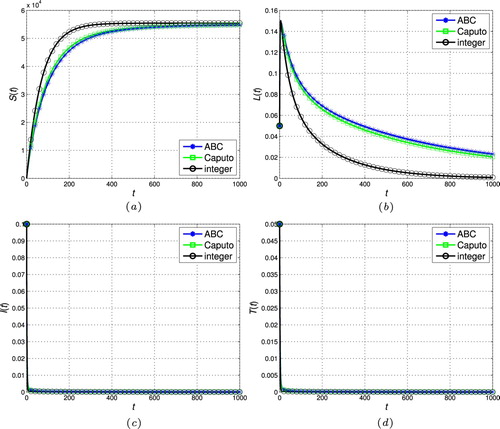
Figure 2. The stability of the disease-free steady-state ($\zeta =0.95$ and $R_0<1$). (a) Susceptible individuals. (b) Latently infected individuals. (c) Actively infectious individuals and (d) under treatment individuals.

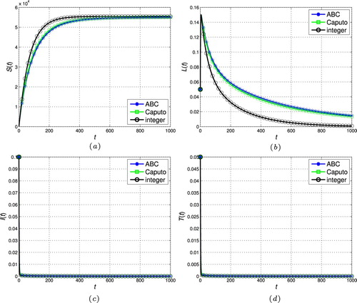
Figure 3. The stability of the disease-free steady-state ($\zeta =0.97$ and $R_0<1$). (a) Susceptible individuals. (b) Latently infected individuals. (c) Actively infectious individuals and (d) under treatment individuals.

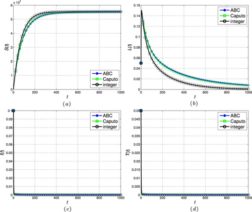
Figure 4. The stability of the disease-free steady-state ($\zeta =0.99$ and $R_0<1$). (a) Susceptible individuals. (b) Latently infected individuals. (c) Actively infectious individuals and (d) under treatment individuals.

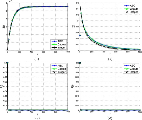
Figure 5. The stability of the endemic stead-state ($\zeta =0.93$ and $R_0>1$). (a) Susceptible individuals. (b) Latently infected individuals. (c) Actively infectious individuals and (d) under treatment individuals.

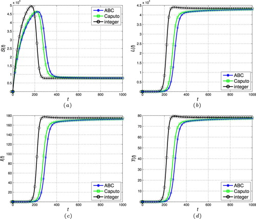
Figure 6. The stability of the endemic stead-state ($\zeta =0.95$ and $R_0>1$). (a) Susceptible individuals. (b) Latently infected individuals. (c) Actively infectious individuals and (d) Under treatment individuals.

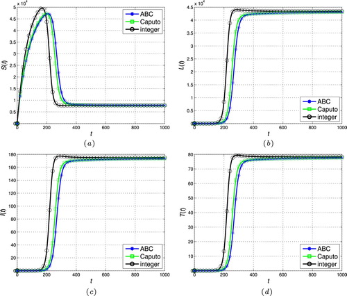
Figure 7. The stability of the endemic stead-state ($\zeta =0.97$ and $R_0>1$). (a) Susceptible individuals. (b) Latently infected individuals. (c) Actively infectious individuals and (d) Under treatment individuals.

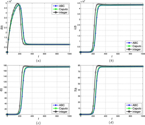
Figure 8. The stability of the endemic stead-state ($\zeta =0.99$ and $R_0>1$). (a) Susceptible individuals. (b) Latently infected individuals. (c) Actively infectious individuals and (d) Under treatment individuals.

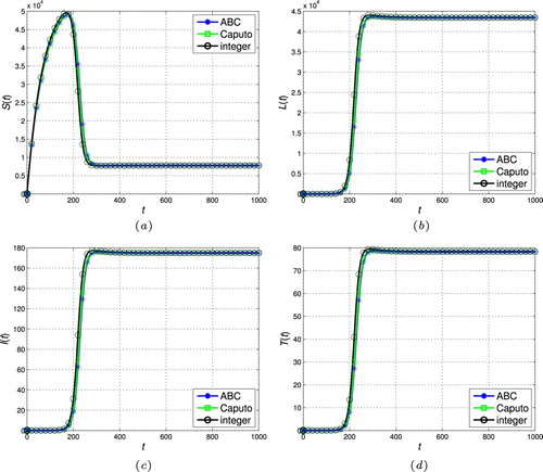
Table 1. The realistic values of parameters.

Parameters	Values
Λ	792.8571 [39]
b	$5\times {10}^{-5}$ [44]
μ	$\frac{1}{70}$ [45]
k	0.15 [39]
δ	1.5 [46]
ϵ	0.00368 [47]
γ	0.7 [39]
$a_1$	0.3 [48]
$a_2$	0.05 [39]

6. Conclusions

The main objective of this research was to investigate a new fractional tuberculosis model involving a nonsingular operator with ML kernel. The proposed model was solved by a new and efficient numerical algorithm based on the PI rule. Numerical results in Figures 1–8 verified the usefulness of employing nonsingular operator to extract different aspects of the considered model compared to the other integer and non-integer order operators. Therefore, the fractional calculus has the potential of providing more flexible models than the classic integer calculus to describe the complex dynamics of the real-world phenomena.

Acknowledgments

This project was funded by the Deanship of Scientific Research (DSR) at King Abdulaziz University, Jeddah, under grant no. G:466-130-1440. The authors, therefore, acknowledge with thanks DSR for technical and financial support.

Disclosure statement

No potential conflict of interest was reported by the authors.

ORCID

Malik Zaka Ullah  http://orcid.org/0000-0003-2944-0352

Abdullah K. Alzahrani  http://orcid.org/0000-0002-1895-3892

Additional information

Funding

This project was funded by the Deanship of Scientific Research (DSR) at King Abdulaziz University, Jeddah, under grant no. G:466-130-1440. The authors, therefore, acknowledge with thanks DSR for technical and financial support.

References

- Magin RL. Fractional calculus in bioengineering. Redding (CT): Begell House; 2006.
- Magin RL. Fractional calculus in bioengineering, part 2. Crit Rev Biomed Eng. 2004;32:105–193.
- Magin RL. Fractional calculus in bioengineering, part 3. Crit Rev Biomed Eng. 2004;32:195–378.
- Pinto CM, Machado JAT. Fractional model for malaria transmission under control strategies. Comput Math Appl. 2013;66:908–916.
- Arshad S, Baleanu D, Huang J, et al. Dynamical analysis of fractional order model of immunogenic tumors. Adv Mech Eng. 2016;8(7):1–13.
- Jajarmi A, Baleanu D. A new fractional analysis on the interaction of HIV with CD4+ T-cells. Chaos Soliton Fract. 2018;113:221–229.
- Carvalho ARM, Pinto CMA, Baleanu D. HIV/HCV coinfection model: a fractional-order perspective for the effect of the HIV viral load. Adv Differ Equ. 2018;2018:2.
- Zaka Ullah M, Al-Aidarous ES, Baleanu D. New aspects of immunogenic tumors within different fractional operators. J Comput Nonlinear Dynam. 2019;14(4):041009.
- World Health Organization. 2018. Available from: http://www.who.int/en/news-room/fact-sheets/detail/tuberculosis
- Silva CJ, Torres DFM. Optimal control of tuberculosis: a review. In: Bourguignon JP, et al., editors. Dynamics, games and science. Berlin: Springer; 2015. p. 701–722. (CIM series in mathematical sciences).
- Denysiuk R, Silva CJ, Torres DFM. Multiobjective approach to optimal control for a tuberculosis model. Optim Methods Softw. 2015;30(5):893–910.
- Silva CJ, Maurer H, Torres DFM. Optimal control of a tuberculosis model with state and control delays. Math Biosci Eng. 2017;14(1):321–337.
- Silva CJ, Torres DFM. Optimal control strategies for tuberculosis treatment: a case study in Angola. Numer Algebra Control Optim. 2012;2(3):601–617.
- Egonmwan AO, Okuonghae D. Analysis of a mathematical model for tuberculosis with diagnosis. J Appl Math Comput. 2019;59(1–2):129–162.
- Kim S, de los Reyes AA, Jung E. Mathematical model and intervention strategies for mitigating tuberculosis in the Philippines. J Theor Biol. 2018;443:100–112.
- Sweilam NH, AL-Mekhlafi SM. Numerical study for multi-strain tuberculosis (TB) model of variable-order fractional derivatives. J Adv Res. 2016;7(2):271–283.
- Wojtak W, Silva CJ, Torres DFM. Uniform asymptotic stability of a fractional tuberculosis model. Math Model Nat Phenom. 2018;13(1):9.
- Khan MA, Ullah S, Farooq M. A new fractional model for tuberculosis with relapse via Atangana–Baleanu derivative. Chaos Soliton Fract. 2018;116:227–238.
- Carvalho ARM, Pinto CMA. Non-integer order analysis of the impact of diabetes and resistant strains in a model for TB infection. Commun Nonlinear Sci. 2018;61:104–126.
- Ullah S, Khan MA, Farooq M. A fractional model for the dynamics of TB virus. Chaos Soliton Fract. 2018;116:63–71.
- Sweilam NH, AL-Mekhlafi SM, Baleanu D. Optimal control for a fractional tuberculosis infection model including the impact of diabetes and resistant strains. J Adv Res. 2019;17:125–137.
- Anukokila P, Radhakrishnan B. Goal programming approach to fully fuzzy fractional transportation problem. J Taibah Univ Sci. 2019;13(1):864–874.
- Mallawi F, Alzaidy JF, Hafez RM. Application of a Legendre collocation method to the space-time variable fractional-order advection-dispersion equation. J Taibah Univ Sci. 2019;13(1):324–330.
- Vivek D, Shah K, Kanagarajan K. Dynamical analysis of Hilfer-Hadamard type fractional pantograph equations via successive approximation. J Taibah Univ Sci. 2019;13(1):225–230.
- Bahaa GM, Hamiaz A. Optimal control problem for coupled time-fractional diffusion systems with final observations. J Taibah Univ Sci. 2019;13(1):124–135.
- Khan U, Ellahi R, Khan R, et al. Extracting new solitary wave solutions of Benny-Luke equation and Phi-4 equation of fractional order by using (G'/G)-expansion method. Opt Quant Electron. 2017;49:362.
- Rahmatullah, Ellahi R, Mohyud-Din ST, et al. Exact traveling wave solutions of fractional order Boussinesq-like equations by applying exp-function method. Res Phys. 2018;8:114–120.
- Sohail A, Maqbool K, Ellahi R. Stability analysis for fractional-order partial differential equations by means of space spectral time Adams-Bashforth Moulton method. Numer Meth Partial Differ Equ. 2018;34(1):19–29.
- Atangana A, Baleanu D. New fractional derivatives with nonlocal and non-singular kernel: theory and application to heat transfer model. Therm Sci. 2016;20(2):763–769.
- Baleanu D, Jajarmi A, Hajipour M. On the nonlinear dynamical systems within the generalized fractional derivatives with Mittag–Leffler kernel. Nonlinear Dyn. 2018;94(1):397–414.
- Korpinar Z, Inc M, Baleanu D, et al. Theory and application for the time fractional Gardner equation with Mittag–Leffler kernel. J Taibah Univ Sci. 2019;13(1):813–819.
- Baleanu D, Sajjadi SS, Jajarmi A, et al. New features of the fractional Euler-Lagrange equations for a physical system within non–singular derivative operator. Eur Phys J Plus. 2019;134:181.
- Yadav S, Pandey RK, Shukla AK. Numerical approximations of Atangana–Baleanu Caputo derivative and its application. Chaos Soliton Fract. 2019;118:58–64.
- Qureshi S, Yusuf A, Shaikh AA, et al. Fractional modeling of blood ethanol concentration system with real data application. Chaos. 2019;29(1):013143.
- Qureshi S, Atangana A. Mathematical analysis of dengue fever outbreak by novel fractional operators with field data. Physica A. 2019;526:121127.
- Marin M, Vlase S, Ellahi R, et al. On the partition of energies for backward in time problem of the thermoelastic materials with a dipolar structure. Symmetry. 2019;11(7):863.
- Marin M, Baleanu D, Carstea C, et al. A uniqueness result for final boundary value problem of microstretch bodies. J Nonlinear Sci App. 2017;10(4):1908–1918.
- Abdeljawad T, Baleanu D. Integration by parts and its applications of a new nonlocal fractional derivative with Mittag–Leffler nonsingular kernel. J Nonlinear Sci Appl. 2017;10:1098–1107.
- Yang Y, Li J, Ma Z, et al. Global stability of two models with incomplete treatment for tuberculosis. Chaos Soliton Fract. 2010;43:79–85.
- Gómez-Aguilar JF, Rosales-García JJ, Bernal-Alvarado JJ, et al. Fractional mechanical oscillators. Revisa Mex Fis. 2012;58:348–352.
- van den Driessche P, Watmough J. Reproduction numbers and subthreshold endemic equilibria for compartmental models of disease transmission. Math Biosci. 2002;180:29–48.
- Ghanbari B, Kumar D. Numerical solution of predator-prey model with Beddington-DeAngelis functional response and fractional derivatives with Mittag-Leffler kernel. Chaos. 2019;29(6):063103.
- Garrappa R. Numerical solution of fractional differential equations: a survey and a software tutorial. Mathematics. 2018;6(2):16.
- Blower SM, McLean AR, Porco TC, et al. The intrinsic transmission dynamics of tuberculosis epidemics. Nat Med. 1995;1:815–821.
- Castillo-Chavez C, Feng Z. To treat or not to treat: the case of tuberculosis. J Math Biol. 1997;35:629–656.
- Rodriguesa P, Gomes MGM, Rebelo C. Drug resistance in tuberculosis – a reinfection model. Theor Popul Biol. 2007;71(2):196–212.
- Castillo-chavez C, Song B. Dynamical models of tuberculosis and their applications. Math Biosci Eng. 2004;1(2):361–404.
- Cohen T, Murray M. Modeling epidemics of multidrug-resistant M. tuberculosis of heterogeneous fitness. Nat Med. 2004;10(10):1117–1121.