Length and curvature variation energy minimizing planar cubic G¹ Hermite interpolation curve

Abstract

In this paper, we study how to construct a planar cubic G¹ Hermite interpolation curve with minimal length and curvature variation energy. This problem is solved by a bi-objective optimization model. We prove that there is a unique solution to this problem and give the expression of the solution. Some numerical examples show that the proposed method makes the curvature variation energy of the curve as small as possible when the length of the curve as short as possible.

KEYWORDS:

• Hermite interpolation curve
• length
• curvature variation energy
• minimization
• bi-objective optimization

MSC:

• 65D07
• 65D05
• 65D17

1. Introduction

It is known that the planar two-point cubic G¹ Hermite interpolation curve can be described as follows, (1) $\begin{array}{rl}\mathbf{b}\left(t\right)& ={\mathbf{p}}_0{B}_0^3\left(t\right)+({\mathbf{p}}_0+\frac{1}{3}{\alpha }_0{\mathbf{d}}_0)B_1^3\left(t\right)\\ & +({\mathbf{p}}_1-\frac{1}{3}{\alpha }_1{\mathbf{d}}_1)B_2^3\left(t\right)+{\mathbf{p}}_1{B}_3^3\left(t\right)\text{,}\end{array}$(1) where ${\mathbf{p}}_0$ and ${\mathbf{p}}_1$ are two points, ${\mathbf{d}}_0$ and ${\mathbf{d}}_1$ are two unit tangent directions, i.e. $||{\mathbf{d}}_0||=||{\mathbf{d}}_1||=1$, ${\alpha }_0$ and ${\alpha }_1$ are positive numbers, $B_k^3\left(t\right)=(3!/k!(3-k)!)t^k(1-t{)}^{3-k}(k=0,1,2,3)$ are cubic Bernstein basis polynomials. In general, the unit tangent directions ${\mathbf{d}}_0$ and ${\mathbf{d}}_1$ are given in advance and the positive numbers ${\alpha }_0$ and ${\alpha }_1$ are often used as free parameters. One can choose suitable ${\alpha }_0$ and ${\alpha }_1$ to make the cubic G¹ Hermite interpolation curve meet some certain needs.

Because the construction of fair (or smooth) curves is a fundamental problem in the filed of CAD and related application fields (see [1–3]), a natural idea is to find the optimal ${\alpha }_0$ and ${\alpha }_1$ for constructing the fair cubic G¹ Hermite interpolation curves. The general ways to construct fair curves are achieved by minimizing some energy functional representing the fairness (see [4]). The strain energy (bending energy) and curvature variation energy are two widely adopted metrics to describe the fairness of a planar curve, since curvature is the universal shape measure for curves (see [1, 5–8]). Recently, some works on determining suitable ${\alpha }_0$ and ${\alpha }_1$ of the planar cubic G¹ Hermite interpolation curve via strain energy minimization or curvature variation energy minimization have been proposed (see [4, 9–12]).

As with fairness, length is another usual shape measure for curves. People often need to construct curves with specific length in the filed of CAD and related application fields. It is not difficult to think that one can find suitable ${\alpha }_0$ and ${\alpha }_1$ to construct a cubic G¹ Hermite curve with required length. Furthermore, one can even find suitable ${\alpha }_0$ and ${\alpha }_1$ to construct a fair cubic G¹ Hermite curve with required length. Unfortunately, there is little discussion on this issue at present. In this paper, we consider finding suitable ${\alpha }_0$ and ${\alpha }_1$ for constructing the planar cubic G¹ Hermite curves with minimal length and curvature variation energy. We give the computing method in Section 2. In Section 3 we show some numerical examples to illustrate the effectiveness of the method. We present a short conclusion and discussion in Section 4.

2. The computing method

2.1. Length minimization

Firstly, we consider minimizing the length of the cubic G¹ Hermite interpolation curve for constructing a curve with minimal length. As we know, the length of the curve $\mathbf{b}\left(t\right)$ can be expressed by (2) $s_1\left(\mathbf{b}\right)={\int }_0^1||{\mathbf{b}}^{\mathrm{\prime }}\left(t\right)||\text{d}t.$(2)

Because it is too complicated for most practical applications, Equation (2) is often simplified to the following approximate form (see [13]), (3) ${\hat{s}}_1\left(\mathbf{b}\right)={\int }_0^1{||{\mathbf{b}}^{\mathrm{\prime }}\left(t\right)||}^{\text{2}}\text{d}t.$(3)

By a deduction from Equation (1), we can obtain that (4) $\begin{array}{rl}{\mathbf{b}}^{\mathrm{\prime }}\left(t\right)& ={\alpha }_0\left(B_0^2\left(t\right)-B_1^2\left(t\right)\right){\mathbf{d}}_0-{\alpha }_1\left(B_1^2\left(t\right)-B_2^2\left(t\right)\right){\mathbf{d}}_1\\ & +3B_1^2\left(t\right)\Delta {\mathbf{p}}_0\text{,}\end{array}$(4) where $\Delta {\mathbf{p}}_0:={\mathbf{p}}_1-{\mathbf{p}}_0$, and $B_k^2\left(t\right)=(2!/k!(2-k)!)t^k(1-t{)}^{2-k}(k=0,1,2)$ are quadratic Bernstein basis polynomials.

By computing from Equation (4), Equation (3) becomes (5) $\begin{array}{rl}{\hat{s}}_1({\alpha }_0,{\alpha }_1)& ={\int }_0^1||{\alpha }_0\left(B_0^2\left(t\right)-B_1^2\left(t\right)\right){\mathbf{d}}_0\\ & -{\alpha }_1\left(B_1^2\left(t\right)-B_2^2\left(t\right)\right){\mathbf{d}}_1+3B_1^2\left(t\right)\Delta {\mathbf{p}}_0|{|}^{\text{2}}\text{d}t\\ & =\frac{1}{15}(2{\alpha }_0^2+2{\alpha }_1^2-{\alpha }_0{\alpha }_1({\mathbf{d}}_0\cdot {\mathbf{d}}_1)\\ & -3{\alpha }_0\left(\Delta {\mathbf{p}}_0\cdot {\mathbf{d}}_0\right)-3{\alpha }_1\left(\Delta {\mathbf{p}}_0\cdot {\mathbf{d}}_1\right)\\ & +18{||\Delta {\mathbf{p}}_0||}^2)\text{,}\end{array}$(5) where $\mathbf{a}\cdot \mathbf{b}:=a_x{b}_x+a_y{b}_y$ denotes the dot product of planar vector.

Let (6) $\begin{array}{rl}{h}_1({\alpha }_0,{\alpha }_1):& =2{\alpha }_0^2+2{\alpha }_1^2-{\alpha }_0{\alpha }_1\left({\mathbf{d}}_0\cdot {\mathbf{d}}_1\right)\\ & -3{\alpha }_0\left(\Delta {\mathbf{p}}_0\cdot {\mathbf{d}}_0\right)-3{\alpha }_1\left(\Delta {\mathbf{p}}_0\cdot {\mathbf{d}}_1\right)\\ & +18||\Delta {\mathbf{p}}_0|{|}^2\text{,}\end{array}$(6) then Equations (5) and (6) have the same minimum.

The gradients of Equation (6) can be calculated as follows, (7) $\left\{\begin{array}{l}\frac{\mathrm{\partial }{h}_1}{\mathrm{\partial }{\alpha }_0}=4{\alpha }_0-\left({\mathbf{d}}_0\cdot {\mathbf{d}}_1\right){\alpha }_1-3\left(\Delta {\mathbf{p}}_0\cdot {\mathbf{d}}_0\right)\text{,}\\ \frac{\mathrm{\partial }{h}_1}{\mathrm{\partial }{\alpha }_1}=4{\alpha }_1-\left({\mathbf{d}}_0\cdot {\mathbf{d}}_1\right){\alpha }_0-3\left(\Delta {\mathbf{p}}_0\cdot {\mathbf{d}}_1\right).\end{array}\right.$(7)

We can see from Equation (7) that the Hessian matrix of $h_1({\alpha }_0,{\alpha }_1)$ is (8) $\begin{array}{rl}{H}_1& =\left(\begin{array}{cc}4& -\left({\mathbf{d}}_0\cdot {\mathbf{d}}_1\right)\\ -\left({\mathbf{d}}_0\cdot {\mathbf{d}}_1\right)& 4\end{array}\right)\\ & =\left(\begin{array}{cc}4& -\cos \theta \\ -\cos \theta & 4\end{array}\right)\text{,}\end{array}$(8) where $\theta$ represents the angle between vectors ${\mathbf{d}}_0$ and ${\mathbf{d}}_1$. It can be easily checked from Equation (8) that the matrix $H_1$ is symmetric positive definite. That means the quadratic functional $h_1({\alpha }_0,{\alpha }_1)$ is strictly convex, and it has a unique global minimum. The following unique global minimum can be solved by $\left(\mathrm{\partial }{h}_1/\mathrm{\partial }{\alpha }_0\right)=0$ and $\left(\mathrm{\partial }{h}_1/\mathrm{\partial }{\alpha }_1\right)=0$,

(9) $\left\{\begin{array}{l}{\alpha }_0^{\left(1\right)}=\frac{1}{16-{\left({\mathbf{d}}_0\cdot {\mathbf{d}}_1\right)}^2}\left(12\left(\Delta {\mathbf{p}}_0\cdot {\mathbf{d}}_0\right)+3\left(\Delta {\mathbf{p}}_0\cdot {\mathbf{d}}_1\right)\left({\mathbf{d}}_0\cdot {\mathbf{d}}_1\right)\right)\text{,}\\ {\alpha }_1^{\left(1\right)}=\frac{1}{16-{\left({\mathbf{d}}_0\cdot {\mathbf{d}}_1\right)}^2}\left(12\left(\Delta {\mathbf{p}}_0\cdot {\mathbf{d}}_1\right)+3\left(\Delta {\mathbf{p}}_0\cdot {\mathbf{d}}_0\right)\left({\mathbf{d}}_0\cdot {\mathbf{d}}_1\right)\right).\end{array}\right.$(9)

Then, we can choose the parameters as Equation (9) for constructing the cubic G¹ Hermite interpolation curve with minimal length.

2.2. Curvature variation energy minimization

Secondly, we consider minimizing the curvature variation energy of the cubic G¹ Hermite interpolation curve for constructing a fair curve. The curvature variation energy of the curve $\mathbf{b}\left(t\right)$ is defined by (see [5]) (10) $s_2\left(\mathbf{b}\right)={\int }_0^1{\left[{\kappa }^{\mathrm{\prime }}\right(t\left)\right]}^2\text{d}t\text{,}$(10) where $\kappa \left(t\right)=\left(||{\mathbf{b}}^{\mathrm{\prime }}\left(t\right)\times {\mathbf{b}}^{\mathrm{\prime }\mathrm{\prime }}\left(t\right)||/||{\mathbf{b}}^{\mathrm{\prime }}\left(t\right)|{|}^3\right)$ represents the curvature of the curve.

In order to simplify the calculation, Equation (10) can be approximated by (see [12]) (11) ${\hat{s}}_2\left(\mathbf{b}\right)={\int }_0^1{||{\mathbf{b}}^{\mathrm{\prime }\mathrm{\prime }\mathrm{\prime }}\left(t\right)||}^2\text{d}t.$(11)

By a deduction from Equation (1), we can obtain that (12) ${\mathbf{b}}^{\mathrm{\prime }\mathrm{\prime }\mathrm{\prime }}\left(t\right)=6({\alpha }_0{\mathbf{d}}_0+{\alpha }_1{\mathbf{d}}_1-2\Delta {\mathbf{p}}_0).$(12)

By computing from Equation (12), Equation (11) becomes (13) $\begin{array}{rl}{\hat{s}}_2({\alpha }_0,{\alpha }_1)& ={\int }_0^1{||6({\alpha }_0{\mathbf{d}}_0+{\alpha }_1{\mathbf{d}}_1-2\Delta {\mathbf{p}}_0)||}^{\text{2}}\text{d}t\\ & =36({\alpha }_0^2+{\alpha }_1^2+2{\alpha }_0{\alpha }_1({\mathbf{d}}_0\cdot {\mathbf{d}}_1)\\ & -4{\alpha }_0\left(\Delta {\mathbf{p}}_0\cdot {\mathbf{d}}_0\right)\\ & -4{\alpha }_1\left(\Delta {\mathbf{p}}_0\cdot {\mathbf{d}}_1\right)+4{||\Delta {\mathbf{p}}_0||}^2).\end{array}$(13)

Let (14) $\begin{array}{rl}{h}_2({\alpha }_0,{\alpha }_1):& ={\alpha }_0^2+{\alpha }_1^2+2{\alpha }_0{\alpha }_1\left({\mathbf{d}}_0\cdot {\mathbf{d}}_1\right)\\ & -4{\alpha }_0\left(\Delta {\mathbf{p}}_0\cdot {\mathbf{d}}_0\right)-4{\alpha }_1\left(\Delta {\mathbf{p}}_0\cdot {\mathbf{d}}_1\right)\\ & +4||\Delta {\mathbf{p}}_0|{|}^2\text{,}\end{array}$(14) then Equations (13) and (14) have the same minimum.

The gradients of (14) can be calculated as follows, (15) $\left\{\begin{array}{l}\frac{\mathrm{\partial }{h}_2}{\mathrm{\partial }{\alpha }_0}=2{\alpha }_0+2\left({\mathbf{d}}_0\cdot {\mathbf{d}}_1\right){\alpha }_1-4\left(\Delta {\mathbf{p}}_0\cdot {\mathbf{d}}_0\right)\text{,}\\ \frac{\mathrm{\partial }{h}_2}{\mathrm{\partial }{\alpha }_1}=2{\alpha }_1+2\left({\mathbf{d}}_0\cdot {\mathbf{d}}_1\right){\alpha }_0-4\left(\Delta {\mathbf{p}}_0\cdot {\mathbf{d}}_1\right).\end{array}\right.$(15)

We can see from Equation (15) that the Hessian matrix of $h_2({\alpha }_0,{\alpha }_1)$ is (16) $H_2=2\left(\begin{array}{cc}1& \left({\mathbf{d}}_0\cdot {\mathbf{d}}_1\right)\\ \left({\mathbf{d}}_0\cdot {\mathbf{d}}_1\right)& 1\end{array}\right)=2\left(\begin{array}{cc}1& \cos \theta \\ \cos \theta & 1\end{array}\right).$(16)

It can be easily checked from Equation (16) that the matrix $H_2$ is symmetric positive definite when ${\mathbf{d}}_0$ is not parallel to ${\mathbf{d}}_1$. In this case the quadratic functional $h_2({\alpha }_0,{\alpha }_1)$ is strictly convex, and it has a unique global minimum. The following unique global minimum can be solved by $\left(\mathrm{\partial }{h}_2/\mathrm{\partial }{\alpha }_0\right)=0$ and $\left(\mathrm{\partial }{h}_2/\mathrm{\partial }{\alpha }_1\right)=0$,

(17) $\left\{\begin{array}{l}{\alpha }_0^{\left(2\right)}=\frac{2}{1-{\left({\mathbf{d}}_0\cdot {\mathbf{d}}_1\right)}^2}\left(\left(\Delta {\mathbf{p}}_0\cdot {\mathbf{d}}_0\right)-\left(\Delta {\mathbf{p}}_0\cdot {\mathbf{d}}_1\right)\left({\mathbf{d}}_0\cdot {\mathbf{d}}_1\right)\right)\text{,}\\ {\alpha }_1^{\left(2\right)}=\frac{2}{1-{\left({\mathbf{d}}_0\cdot {\mathbf{d}}_1\right)}^2}\left(\left(\Delta {\mathbf{p}}_0\cdot {\mathbf{d}}_1\right)-\left(\Delta {\mathbf{p}}_0\cdot {\mathbf{d}}_0\right)\left({\mathbf{d}}_0\cdot {\mathbf{d}}_1\right)\right).\end{array}\right.$(17)

Then, we can choose the parameters as Equation (17) for constructing the cubic G¹ Hermite interpolation curve with minimal curvature variation energy.

2.3. Length and curvature variation energy minimization

Finally, let us consider minimizing the length and curvature variation energy synchronously for constructing a fair curve with minimal length. In order to achieve this goal, we need to solve the following bi-objective optimization problem, (18) $\text{min}(h_1({\alpha }_0,{\alpha }_1),h_2({\alpha }_0,{\alpha }_1){)}^{\text{T}}\text{,}$(18) where $h_1({\alpha }_0,{\alpha }_1)$ and $h_2({\alpha }_0,{\alpha }_1)$ is expressed in (6) and (14) respectively.

By taking the sum of the two objectives with weights as a single objective functional, Equation (18) becomes (19) $minh({\alpha }_0,{\alpha }_1,\lambda )=\lambda h_1({\alpha }_0,{\alpha }_1)+(1-\lambda )h_2({\alpha }_0,{\alpha }_1)\text{,}$(19) where $\lambda$ is the weight and $0<\lambda <1$.

If we have determined the value of the weight $\lambda$, the gradients of Equation (19) could be calculated as follows, (20) $\left\{\begin{array}{l}\frac{\mathrm{\partial }h}{\mathrm{\partial }{\alpha }_0}=\lambda \frac{\mathrm{\partial }{h}_1}{\mathrm{\partial }{\alpha }_0}+(1-\lambda )\frac{\mathrm{\partial }{h}_2}{\mathrm{\partial }{\alpha }_0}=2(1+\lambda ){\alpha }_0\\ +(2-3\lambda )\left({\mathbf{d}}_0\cdot {\mathbf{d}}_1\right){\alpha }_1+(\lambda -4)\left(\Delta {\mathbf{p}}_0\cdot {\mathbf{d}}_0\right)\text{,}\\ \frac{\mathrm{\partial }h}{\mathrm{\partial }{\alpha }_1}=\lambda \frac{\mathrm{\partial }{h}_1}{\mathrm{\partial }{\alpha }_1}+(1-\lambda )\frac{\mathrm{\partial }{h}_2}{\mathrm{\partial }{\alpha }_1}=2(1+\lambda ){\alpha }_1\\ +(2-3\lambda )\left({\mathbf{d}}_0\cdot {\mathbf{d}}_1\right){\alpha }_0+(\lambda -4)\left(\Delta {\mathbf{p}}_0\cdot {\mathbf{d}}_1\right).\end{array}\right.$(20)

In this case, we can see from Equation (20) that the Hessian matrix of $h({\alpha }_0,{\alpha }_1)$ is $H=\left(\begin{array}{cc}2(1+\lambda )& (2-3\lambda )\left({\mathbf{d}}_0\cdot {\mathbf{d}}_1\right)\\ (2-3\lambda )\left({\mathbf{d}}_0\cdot {\mathbf{d}}_1\right)& 2(1+\lambda )\end{array}\right).$

Lemma 2.1:

Let ${\mathbf{d}}_0$ be not parallel to ${\mathbf{d}}_1$, the matrix $H$ is symmetric positive definite when $0<\lambda <1$.

Proof: When $0<\lambda <1$, we have $2(1+\lambda )>0$. The determinant of $H$ can be calculated by (21) $\text{det}\left(H\right)=4(1+\lambda {)}^2-(2-3\lambda {)}^2{\cos }^2\theta .$(21) When $0<\lambda <1$, it can be easily checked that $4<4(1+\lambda {)}^2<16$ and $1<(2-3\lambda {)}^2<4$. From (21), we have $\text{det}\left(H\right)>4-4{\cos }^2\theta$. Since ${\mathbf{d}}_0$ is not parallel to ${\mathbf{d}}_1$, we obtain that $\text{det}\left(H\right)>0$. Thus, the matrix $H$ is symmetric positive definite.

Theorem 2.1:

When $0<\lambda <1$ and ${\mathbf{d}}_0$ is not parallel to ${\mathbf{d}}_1$, Equation (19) has a unique global solution given by (22) $\left\{\begin{array}{l}{\alpha }_0=\frac{2(1+\lambda )(4-\lambda )\left(\Delta {\mathbf{p}}_0\cdot {\mathbf{d}}_0\right)-(2-3\lambda )(4-\lambda )\left(\Delta {\mathbf{p}}_0\cdot {\mathbf{d}}_1\right)\left({\mathbf{d}}_0\cdot {\mathbf{d}}_1\right)}{4{(1+\lambda )}^2-{(2-3\lambda )}^2{\left({\mathbf{d}}_0\cdot {\mathbf{d}}_1\right)}^2}\text{,}\\ {\alpha }_1=\frac{2(1+\lambda )(4-\lambda )\left(\Delta {\mathbf{p}}_0\cdot {\mathbf{d}}_1\right)-(2-3\lambda )(4-\lambda )\left(\Delta {\mathbf{p}}_0\cdot {\mathbf{d}}_0\right)\left({\mathbf{d}}_0\cdot {\mathbf{d}}_1\right)}{4{(1+\lambda )}^2-{(2-3\lambda )}^2{\left({\mathbf{d}}_0\cdot {\mathbf{d}}_1\right)}^2}.\end{array}\right.$(22)

Proof: According to Lemma 1, Equation (19) has a unique global solution that can be solved by $\left(\mathrm{\partial }h/\mathrm{\partial }{\alpha }_0\right)=0$ and $\left(\mathrm{\partial }h/\mathrm{\partial }{\alpha }_1\right)=0$. By computing from Equation (20), we can obtain the unique global solution expressed in Equation (22).

Then, we can choose the parameters as Equation (22) for constructing the cubic G¹ Hermite interpolation curve with minimal length and curvature variation energy.

Now, the only task left is to determine the value of the weight $\lambda$ in Equation (22). There are several approaches to determine the value of the weight (see [14]). Here, we use the ranking method. The overall algorithm is described in Algorithm 1, with some key steps detailed below. In Line 1, we compute the deviation between the two target functions. It is obvious that the deviation ${\delta }_i^{\left(j\right)}\ge 0$, $i,j=1,2$. In Line 2, we compute the average deviation of the two target functions. Since ${\delta }_i^{\left(i\right)}=0$, the average deviations are actually $m_1={\delta }_1^{\left(2\right)}$ and $m_2={\delta }_2^{\left(1\right)}$. In Line 3, we compute the initial weights of the two target functions. It is obvious that the initial weights satisfy ${\lambda }_1,{\lambda }_2\ge 0$ and ${\lambda }_1+{\lambda }_2=1$. In Line 4, we choose the smaller weight for the objective function with larger average deviation, and the larger weight for the objective function with smaller average deviation.

Table

Algorithm 1: Determining the weight $\lambda$ by ranking method.
1: Compute ${\delta }_i^{\left(j\right)}:=h_i({\alpha }_0^{\left(j\right)},{\alpha }_1^{\left(j\right)})-h_i({\alpha }_0^{\left(i\right)},{\alpha }_1^{\left(i\right)})$, $i,j=1,2$, where $({\alpha }_0^{\left(i\right)},{\alpha }_1^{\left(i\right)})$ is the solution of single objective problem $min{h}_i({\alpha }_0,{\alpha }_1)$, $i=1,2$.
2: Let $m_i:={\sum }_{j=1}^2{\delta }_i^{\left(j\right)}$, $i=1,2$.
3: Compute ${\lambda }_i=m_i/(m_1+m_2)$, $i=1,2$.
4: If ${\lambda }_1\ge {\lambda }_2$, the weight is taken as $\lambda ={\lambda }_2$; else, the weight is taken as $\lambda ={\lambda }_1$.

3. Numerical examples

In this section, we give some numerical examples to illustrate effectiveness of the length and curvature variation energy minimization, and compare this method with the length minimization and the curvature variation energy minimization. All the numerical examples are implemented by MATLAB.

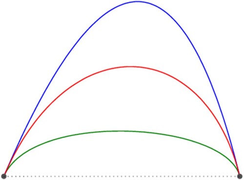
Example 3.1:

Let us take the following data, $\begin{array}{rl}{\mathbf{p}}_0& =(-1,0)\text{,}{\mathbf{p}}_1=(1,0)\text{,}{\mathbf{d}}_0=(\cos \pi /4,\sin \pi /4)\text{,}\\ {\mathbf{d}}_1& =(\cos \pi /3,-\sin \pi /3).\end{array}$We can obtain the two parameters of the three methods from Equations (9), (17), (22) and Algorithm 1. By substituting the obtained parameters into Equations (5) and (13), we can get the length and the curvature variation energy of the three methods. For the convenience of comparison, we put these results in Table 1.

Table 1. Parameters, length and curvature variation energy of the three methods (Example 1).

Method	Parameters	length	Curvature variation energy
Length minimization	(1.0164, 0.6842)	4.5878	311.5705
Curvature variation energy minimization	(3.5863, 2.9282)	6.2393	0
Length and curvature variation energy minimization	(2.3249, 1.7782)	5.0004	77.8611

Figure 1 shows the graphs of the following curves: the cubic Hermite interpolation curve with minimal length (in green), the cubic Hermite interpolation curve with minimal curvature variation energy (in blue), the cubic Hermite interpolation curve with minimal length and curvature variation energy (in red), and the polygonal line joining the points (in dotted).

Figure 1. The graphs of the curves (Example 1).

Example 3.2:

Let us take the following data, $\begin{array}{rl}{\mathbf{p}}_0& =(-1,0)\text{,}{\mathbf{p}}_1=(1,0)\text{,}{\mathbf{d}}_0=(\cos \pi /4,\sin \pi /5)\text{,}\\ {\mathbf{d}}_0& =(\cos \pi /4,\sin \pi /5).\end{array}$We put the results of the parameters, length and the curvature variation energy of the three methods in Table 2.

In Figure 2 we present the cubic Hermite interpolation curve with minimal length (in green), the cubic Hermite interpolation curve with minimal curvature variation energy (in blue), the cubic Hermite interpolation curve with minimal length and curvature variation energy (in red), and the polygonal line joining the points (in dotted).

Example 3.3:

We take the following data taken from a unit arc, ${\mathbf{p}}_i=(\sin {\theta }_i,\cos {\theta }_i)\text{,}{\mathbf{d}}_i=(\cos {\theta }_i,-\sin {\theta }_i)\text{,}$where ${\theta }_i=\pi /4,\pi /2,2\pi /3$. In this case, the G¹ Hermite interpolation curve consists of two segments (The two segments are named as s1 and s2 for short). We put the results of the parameters, length and the curvature variation energy of each segment of the three methods in Table 3.

The cubic Hermite interpolation curve with minimal length (in green), the cubic Hermite interpolation curve with minimal curvature variation energy (in blue), the cubic Hermite interpolation curve with minimal length and curvature variation energy (in red), and the unit arc (in dotted) are shown in Figure 3.

Figure 2. The graphs of the curves (Example 2).

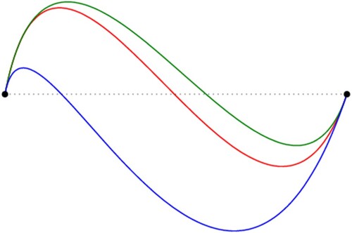
Figure 3. The graphs of the curves (Example 3).

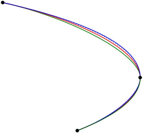
Table 2. Parameters, length and curvature variation energy of the three methods (Example 2).

Method	Parameters	length	Curvature variation energy
Length minimization	(1.3563, 1.4838)	4.3681	189.0343
Curvature variation energy minimization	(0.6834, 2.6914)	4.6661	138.3666
Length and curvature variation energy minimization	(1.3659, 1.8918)	4.3901	165.3203

Table 3. Parameters, length and curvature variation energy of each segment of the three methods.

	Parameters		Length		Curvature variation energy
Method	s1	s2	s1	s2	s1	s2
Length minimization	(0.6442, 0.6442)	(0.4786, 0.4786)	0.6118	0.2737	4.1710	0.4407
Curvature variation energy minimization	(0.8284, 0.8284)	(0.5359, 0.5359)	0.6193	0.2744	4.4373e-31	3.2171e-30
Length and curvature variation energy minimization	(0.7397, 0.7397)	(0.5122, 0.5122)	0.6138	0.2739	0.9687	0.0754

The above numerical examples show that the proposed method makes the curvature variation energy of the curve as small as possible when the length of the curve as short as possible. If we need to construct the fair curves with minimal length, the proposed method will come in handy.

4. Conclusion and discussion

This paper focuses on how to construct a fair cubic G¹ Hermite interpolation curve with minimal length, which is achieved by solving a bi-objective optimization problem to search the optimal values of the two parameters. It can be found that there is a unique solution to this problem, and the expression of the solution is given in this paper. The cubic G¹ Hermite interpolation curves obtained by the proposed method have less curvature variation energy in the case of shorter length. Some numerical examples verify this conclusion.

In this paper, we use the curvature variation energy as the metric to construct a fair cubic G¹ Hermite interpolate curve. In fact, the strain energy is also a metric to construct fair curves. Maybe we can replace the curvature variation energy minimization with the strain energy minimization in the proposed method; however, the curvature variation energy minimization may obtain more satisfactory results in shape and fairness than the strain energy minimization for constructing cubic G¹ Hermite interpolation curves (see [4]). In addition, it is necessary to impose a feasible region on the two parameters (i.e.$\{({\alpha }_0,{\alpha }_1)\in {\mathbb{R}}^2|{\alpha }_0>0,{\alpha }_1>0\}$) for constructing a cubic G¹ Hermite interpolation curve (see [4, 10–12]). Therefore, one should select appropriate G¹ Hermite data when using the proposed method.

Disclosure statement

No potential conflict of interest was reported by the authors.

Additional information

Funding

This work is supported by the Scientific Research Fund of Hunan Provincial Education Department under the [grant number 18A415], and the Open Research Fund Program of Data Recovery Key Laboratory of Sichuan Province under the [grant number DRN19019].

References

- Farin G. Curves and surfaces for CAGD: a practical guide. San Diego: Academic Press; 2002.
- Hofer M, Pottmann H. Energy-minimizing splines in manifolds. ACM T Graphic. 2004;23:284–293. doi: 10.1145/1015706.1015716
- Fan W, Lee C, Chen J. A realtime curvature-smooth interpolation scheme and motion planning for CNC machining of short line segments. Int J Mach Tool Manu. 2015;96:27–46. doi: 10.1016/j.ijmachtools.2015.04.009
- Lu L, Jiang C, Hu Q. Planar cubic G1 and quintic G2 Hermite interpolations via curvature variation minimization. Comput Graph. 2018;70:92–98. doi: 10.1016/j.cag.2017.07.007
- Farin G. Geometric Hermite interpolation with circular precision. Comput Aided Geom D. 2008;40:476–479. doi: 10.1016/j.cad.2008.01.003
- Renka R. Shape-preserving interpolation by fair discrete G3 space curves. Comput Aided Geom D. 2005;22:793–809. doi: 10.1016/j.cagd.2005.03.003
- Xu G, Wang G, Chen W. Geometric construction of energy-minimizing Bézier curves. Sci China Inform Sci. 2011;54:1395–1406. doi: 10.1007/s11432-011-4294-8
- Ahn Y, Hoffmann C, Rosen P. Geometric constraints on quadratic Bézier curves using minimal length and energy. J Comput Appl Math. 2014;255:887–897. doi: 10.1016/j.cam.2013.07.005
- Yong J, Cheng F. Geometric Hermite curves with minimum strain energy. Comput Aided Geom D. 2004;21:281–301. doi: 10.1016/j.cagd.2003.08.003
- Jaklič G, Žagar E. Planar cubic G1 interpolatory splines with small strain energy. J Comput Appl Math. 2011;235:2758–2765. doi: 10.1016/j.cam.2010.11.025
- Jaklič G, Žagar E. Curvature variation minimizing cubic Hermite interpolants. Appl Math Comput. 2011;218:3918–3924.
- Lu L. A note on curvature variation minimizing cubic Hermite interpolants. Appl Math Comput. 2015;259:596–599.
- Veltkamp R, Wesselink W. Modeling 3D curves of minimal energy. In: Eurographics 95, Maastricht, Netherlands, 1995;97–110.
- Lin C, Dong J. The methods and theories of multi-objective optimizations. Changchun: Jilin Education Press; 1992.