Constructions of the optical solitons and other solitons to the conformable fractional Zakharov–Kuznetsov equation with power law nonlinearity

Abstract

The current research manifests kink wave answers, mixed singular optical solitons, the mixed dark-bright lump answer, the mixed dark-bright periodic wave answer, and periodic wave answers to the conformable fractional ZK model, including power law nonlinearity by plugging the revised $\left(G^{\prime }/G\right)$-expansion process. The constraint requirements for the occurrence of substantial solitons are provided. Under the selection of proper values of a, b, n, t, λ, μ and α, the 2D and 3D pictures to a few of the recorded answers are sketched. From our obtained solutions, we might decide that the investigated procedure is hugely muscular, sincere, and essential in rendering various new soliton solutions of distinct nonlinear conformable fractional evolution equations and accordingly, we shall bring it up in our future investigations.

Keywords:

• Modified $\left(G^{\prime }/G\right)$-expansion method
• $(3+1)$-dimensional conformable fractional Zakharov–Kuznetsov equation with power law nonlinearity
• conformable fractional derivative
• travelling wave solutions
• soliton solutions

2010 AMS (MOS) Subject Classifications:

• 35C07
• 35C08
• 35Q53

1. Introduction

Nowadays, the study of closed-form wave answers the nonlinear wave equation improvement ahead of its measurement. Besides, a conformable derivative nonlinear ordinary differential equation has been converted mostly to make their application in the communication scheme. Accordingly, the problem of securing the closed-form wave answers of the conformable nonlinear model attracts a lot of consideration. Nonetheless, numerous applications have been executed in the economy, quantum field theory, optical fibres, plasma physics, fluid mechanics, mathematical physics, biology, geochemistry, to mention a few. Thus, various mathematical methods have been improved to answer them, such as Lie symmetry analysis [1], the auxiliary equation method [2], the FRDTM [3], the tan$\phi \left(\xi \right)/2)$-expansion method [4], Tanh method [5], the Riccati–Bernoulli sub-ODE method [6], the exp$-\phi \left(\xi \right)$-expansion method [7–9], extended trial equation method [10], Fractional Fan sub-equation method [11], new generalized $\left(G^{\prime }/G\right)$-expansion method [12–15], exponential rational function method [16], $\left(G^{\prime }/G\right)$-expansion method [17–19], modified extended tanh method [20], improved $\left(G^{\prime }/G\right)$-expansion method [21], differential transform method [22], the Painleve analysis [23], fractional homotopy method [24], Truncation method [25], Semi-Inverse variational principle [26], the Feng's first integral method [27], the unified method [28], $\left(\frac{G^{\prime }}{G^2}\right)$-expansion method [29], singular manifold method [30], singular manifold method [31], homotopy perturbation transform method [32], Collocation method [33], separation of variables method [34], Lagrange multiplier method [35], fractional Adams– Bashforth–Moulton method [36], Chebyshev wavelet method [37], Jacobi elliptic function method [38], Kudryashov method [39], exp-function method [40], sub-equation method [41], space spectral time-fractional Adam–Bashforth– Moulton method [42], exp-function method [43], the phase field method [44], fractional homotopy analysis transform method [45] and many more [57].

In this paper, the modified $\left(G^{\prime }/G\right)$-expansion process will obtain soliton answers of the following conformable fractional ZK model, including power law nonlinearity [28,46]. We are considering that using above model [28,46], (1) $\begin{array}{r}\frac{{\mathrm{\partial }}^{\alpha }u}{\mathrm{\partial }{t}^{\alpha }}+a{u}^n\frac{\mathrm{\partial }u}{\mathrm{\partial }x}+b\frac{\mathrm{\partial }}{\mathrm{\partial }x}\left(\frac{{\mathrm{\partial }}^{2}u}{\mathrm{\partial }{x}^2}+\frac{{\mathrm{\partial }}^{2}u}{\mathrm{\partial }{y}^2}+\frac{{\mathrm{\partial }}^{2}u}{\mathrm{\partial }{z}^2}\right)=0,\end{array}$(1) where a and b are constants, n is the power law nonlinearity parameter, $\frac{{\mathrm{\partial }}^{\alpha }u}{\mathrm{\partial }{t}^{\alpha }}$ is the evolution term, $u^n\frac{\mathrm{\partial }u}{\mathrm{\partial }x}$ is the nonlinearity and $\frac{\mathrm{\partial }}{\mathrm{\partial }x}\left(\frac{{\mathrm{\partial }}^{2}u}{\mathrm{\partial }{x}^2}+\frac{{\mathrm{\partial }}^{2}u}{\mathrm{\partial }{y}^2}+\frac{{\mathrm{\partial }}^{2}u}{\mathrm{\partial }{z}^2}\right)$ is dispersion. Solitons are the outcome of a rule between dispersion and nonlinearity. The above model typically appears in the analysis of plasma physics. Matebese et al. [46] noted the above model through the three analytical methods, such as the $\left(G^{\prime }/G\right)$-expansion method, the extended tanh function method, and the ansatz method. Besides, Aminikhah et al. [47] attempted to discover the same model when $\alpha =1$ plugging the functional variable method. The particular case where n = 1 and $\alpha =1$ provides the $(3+1)$-dimensional Zakharov–Kuznetsov equation. Section 2 provides a few fundamental aspects and the knowledge of the conformable fractional calculus theory. The novel closed-form wave answers of the recommended model are discussed in Section 4. The last section conveys the conclusions and future tasks.

2. Conformable fractional derivative

This section gives a few essential characteristics and the knowledge of the conformable fractional calculus theory which can be seen in  [48–55].

Definition 2.1

we consider that $f:(0,\mathrm{\infty })\to \mathbb{R}$, therefore, the conformable fractional derivative of f of order α is expressed as (2) $\begin{array}{r}{}_t{D}^{\alpha }f\left(t\right)=\underset{ϵ\to 0}{lim}\frac{f(t+ϵt^{1-\alpha })-f\left(t\right)}{ϵ},\end{array}$(2) for all t>0, $\alpha \in (0,1).$

If f is α-differentiable in some $(0,a),a>0$ and $\underset{t\to 0^{+}}{lim}{(}_t{D}^{\alpha }f\left(t\right))$ exists, then in accordance with the definition, we obtain (3) $\begin{array}{r}{}_t{D}^{\alpha }\left(f\right)\left(0\right)=\underset{t\to 0^{+}}{lim}{(}_t{D}^{\alpha }f\left(t\right)).\end{array}$(3)

The novel definition convinces the characteristics manifested in the following theorem.

Theorem 2.2

We consider that $\alpha \in (0,1]$, and f, g be α-differentiable at a point t, such that

• ${}_t{D}^{\alpha }(af+bg)=a{(}_t{D}^{\alpha }f)+b{(}_t{D}^{\alpha }g),\mathrm{\forall }a,b\in \mathbb{R}$.

• ${}_t{D}^{\alpha }\left(t^{\mu }\right)=\mu t^{\mu -\alpha },forall\mu \in \mathbb{R}.$

• ${}_t{D}^{\alpha }(f+g)=f{(}_t{D}^{\alpha }g)+g{(}_t{D}^{\alpha }f).$

• ${}_t{D}^{\alpha }\left(\frac{f}{g}\right)=\frac{g{(}_t{D}^{\alpha }f)-f{(}_t{D}^{\alpha }g)}{g^2}.$

In addition, if f is differentiable, then ${}_t{D}^{\alpha }f\left(t\right)=t^{1-\alpha }\frac{df}{dt}.$

Abdeljawad [50] established the chain rule under the conformable fractional derivatives.

Theorem 2.3

We consider that $f:(0,\mathrm{\infty })\to \mathbb{R}$ is a function, for example, f is differentiable and also α-differentiable. Let us consider that g is a function defined in the range of f and also differentiable. Then one has the following rule: (4) $\begin{array}{r}{}_t{D}^{\alpha }f\left(fog\right)\left(t\right)=t^{1-\alpha }{g}^{\prime }\left(t\right)f^{\prime }\left(g\right(t\left)\right).\end{array}$(4)

2.1. The fractional complex transformation

This section implements the complex fractional transformation for the fractional-order PDE: (5) $\begin{array}{r}L\left(u,\frac{{\mathrm{\partial }}^{\alpha }u}{\mathrm{\partial }{t}^{\alpha }},\frac{\mathrm{\partial }u}{\mathrm{\partial }x},\frac{\mathrm{\partial }u}{\mathrm{\partial }y},\frac{{\mathrm{\partial }}^{2\alpha }u}{\mathrm{\partial }{t}^{2\alpha }},\frac{{\mathrm{\partial }}^{2}u}{\mathrm{\partial }{t}^2}\right)=0,t\ge 0,0<\alpha \le 1,\end{array}$(5) where $L=u(x,y,t)$. For Equation (5(5) $\begin{array}{r}L\left(u,\frac{{\mathrm{\partial }}^{\alpha }u}{\mathrm{\partial }{t}^{\alpha }},\frac{\mathrm{\partial }u}{\mathrm{\partial }x},\frac{\mathrm{\partial }u}{\mathrm{\partial }y},\frac{{\mathrm{\partial }}^{2\alpha }u}{\mathrm{\partial }{t}^{2\alpha }},\frac{{\mathrm{\partial }}^{2}u}{\mathrm{\partial }{t}^2}\right)=0,t\ge 0,0<\alpha \le 1,\end{array}$(5) ), let $u=u\left(\xi \right)=u(x,y,z,t),\xi =x+y+z-V\frac{t^{\alpha }}{\alpha }$ and obtain $\frac{{\mathrm{\partial }}^{\alpha }}{\mathrm{\partial }{t}^{\alpha }}=-V\frac{\mathrm{\partial }}{\mathrm{\partial }\xi }$, $\frac{\mathrm{\partial }}{\mathrm{\partial }x}=\frac{\mathrm{\partial }}{\mathrm{\partial }\xi }$, $\frac{\mathrm{\partial }}{\mathrm{\partial }y}=\frac{\mathrm{\partial }}{\mathrm{\partial }\xi }$, $\frac{{\mathrm{\partial }}^{2\alpha }}{\mathrm{\partial }{t}^{2\alpha }}=V^2\frac{{\mathrm{\partial }}^2}{\mathrm{\partial }{\xi }^2}$ $\dots$, where V stands for the travelling wave speed. Then, Equation (5(5) $\begin{array}{r}L\left(u,\frac{{\mathrm{\partial }}^{\alpha }u}{\mathrm{\partial }{t}^{\alpha }},\frac{\mathrm{\partial }u}{\mathrm{\partial }x},\frac{\mathrm{\partial }u}{\mathrm{\partial }y},\frac{{\mathrm{\partial }}^{2\alpha }u}{\mathrm{\partial }{t}^{2\alpha }},\frac{{\mathrm{\partial }}^{2}u}{\mathrm{\partial }{t}^2}\right)=0,t\ge 0,0<\alpha \le 1,\end{array}$(5) ) becomes (6) $\begin{array}{r}Q\left(u,\frac{\mathrm{\partial }u}{\mathrm{\partial }\xi },\frac{{\mathrm{\partial }}^{2}u}{\mathrm{\partial }{\xi }^2},\dots \right)=0.\end{array}$(6)

3. New soliton solutions for the $(3+1)$-dimensional conformable fractional Zakharov–Kuznetsov equation with power law nonlinearity

To represent the idea of the modified $\left(G^{\prime }/G\right)$-expansion method [56], we apply the way on the (3 + 1)-dimensional conformable fractional Zakharov–Kuznetsov equation with power law nonlinearity [28,46]. Let us consider that (7) $\begin{array}{r}\frac{{\mathrm{\partial }}^{\alpha }u}{\mathrm{\partial }{t}^{\alpha }}+a{u}^n\frac{\mathrm{\partial }u}{\mathrm{\partial }x}+b\frac{\mathrm{\partial }}{\mathrm{\partial }x}\left(\frac{{\mathrm{\partial }}^{2}u}{\mathrm{\partial }{x}^2}+\frac{{\mathrm{\partial }}^{2}u}{\mathrm{\partial }{y}^2}+\frac{{\mathrm{\partial }}^{2}u}{\mathrm{\partial }{z}^2}\right)=0.\end{array}$(7) Let (8) $\begin{array}{r}u=u\left(\xi \right)=u(x,y,z,t),\xi =x+y+z-V\frac{t^{\alpha }}{\alpha }.\end{array}$(8) From Equations (7(7) $\begin{array}{r}\frac{{\mathrm{\partial }}^{\alpha }u}{\mathrm{\partial }{t}^{\alpha }}+a{u}^n\frac{\mathrm{\partial }u}{\mathrm{\partial }x}+b\frac{\mathrm{\partial }}{\mathrm{\partial }x}\left(\frac{{\mathrm{\partial }}^{2}u}{\mathrm{\partial }{x}^2}+\frac{{\mathrm{\partial }}^{2}u}{\mathrm{\partial }{y}^2}+\frac{{\mathrm{\partial }}^{2}u}{\mathrm{\partial }{z}^2}\right)=0.\end{array}$(7) ) and (8(8) $\begin{array}{r}u=u\left(\xi \right)=u(x,y,z,t),\xi =x+y+z-V\frac{t^{\alpha }}{\alpha }.\end{array}$(8) ), we achieve: (9) $\begin{array}{r}-V\frac{\mathrm{\partial }u}{\mathrm{\partial }\xi }+a{u}^n\frac{\mathrm{\partial }u}{\mathrm{\partial }\xi }+b\frac{\mathrm{\partial }}{\mathrm{\partial }\xi }\left(\frac{{\mathrm{\partial }}^{2}u}{\mathrm{\partial }{\xi }^2}+\frac{{\mathrm{\partial }}^{2}u}{\mathrm{\partial }{\xi }^2}+\frac{{\mathrm{\partial }}^{2}u}{\mathrm{\partial }{\xi }^2}\right)=0.\end{array}$(9) Integrating the above equation, we have (10) $\begin{array}{r}-Vu+\frac{a}{n+1}{u}^{n+1}+3b\frac{{\mathrm{\partial }}^{2}u}{\mathrm{\partial }{\xi }^2}=0.\end{array}$(10) Plugging $u=v^{\frac{1}{n}}$, Equation (10(10) $\begin{array}{r}-Vu+\frac{a}{n+1}{u}^{n+1}+3b\frac{{\mathrm{\partial }}^{2}u}{\mathrm{\partial }{\xi }^2}=0.\end{array}$(10) ) becomes (11) $\begin{array}{rl}& 3bn(n+1)v\frac{{\mathrm{\partial }}^{2}v}{\mathrm{\partial }{\xi }^2}+3b(n^2-1){\left(\frac{\mathrm{\partial }v}{\mathrm{\partial }\xi }\right)}^2\\ & -n^2(1+n)V{v}^2+a{n}^2{v}^3=0,n\ne 0,\pm 1.\end{array}$(11) In accordance with the modified $\left(G^{\prime }/G\right)$-expansion method [56], by plugging homogeneous balance rule between $v\frac{{\mathrm{\partial }}^{2}v}{\mathrm{\partial }{\xi }^2}$ and $v^3$ from the equation (11(11) $\begin{array}{rl}& 3bn(n+1)v\frac{{\mathrm{\partial }}^{2}v}{\mathrm{\partial }{\xi }^2}+3b(n^2-1){\left(\frac{\mathrm{\partial }v}{\mathrm{\partial }\xi }\right)}^2\\ & -n^2(1+n)V{v}^2+a{n}^2{v}^3=0,n\ne 0,\pm 1.\end{array}$(11) ), it yields M = 2. Therefore, Equation (11(11) $\begin{array}{rl}& 3bn(n+1)v\frac{{\mathrm{\partial }}^{2}v}{\mathrm{\partial }{\xi }^2}+3b(n^2-1){\left(\frac{\mathrm{\partial }v}{\mathrm{\partial }\xi }\right)}^2\\ & -n^2(1+n)V{v}^2+a{n}^2{v}^3=0,n\ne 0,\pm 1.\end{array}$(11) ) reduces to (12) $\begin{array}{r}v\left(\xi \right)=A_2{F}^2+A_{1}F+A_0+A_{-1}{F}^{-1}+A_{-2}{F}^{-2},\end{array}$(12) where $A_0$, $A_1$, $A_2$, $A_{-1}$ and $A_{-2}$ are constants.

Plugging Equation (12(12) $\begin{array}{r}v\left(\xi \right)=A_2{F}^2+A_{1}F+A_0+A_{-1}{F}^{-1}+A_{-2}{F}^{-2},\end{array}$(12) ) into Equation (11(11) $\begin{array}{rl}& 3bn(n+1)v\frac{{\mathrm{\partial }}^{2}v}{\mathrm{\partial }{\xi }^2}+3b(n^2-1){\left(\frac{\mathrm{\partial }v}{\mathrm{\partial }\xi }\right)}^2\\ & -n^2(1+n)V{v}^2+a{n}^2{v}^3=0,n\ne 0,\pm 1.\end{array}$(11) ) and then calculating each coefficients of $F^i(\pm 1,\pm 2,\dots \dots .,\pm m)$ to zeros, we obtain the following relations:

• Phase 1: Let $V=-\frac{3b({\lambda }^{2}n-4\mu n-n+1)}{n^2},A_0=\frac{3b({\lambda }^2-4\mu )(n+1)}{2an},A_1=0,A_2=0,A_{-1}=0$, and $A_{-2}=-\frac{9b({\lambda }^4-8{\lambda }^2\mu +16{\mu }^2)(n+1)}{8an}$ and use the values of the Phase 1 into Equation (12(12) $\begin{array}{r}v\left(\xi \right)=A_2{F}^2+A_{1}F+A_0+A_{-1}{F}^{-1}+A_{-2}{F}^{-2},\end{array}$(12) ), we obtain: $\begin{array}{rl}{u}_{11}(x,t)& =\left[\frac{-3b({\lambda }^2-4\mu )(n+1)}{2an}\right.\\ & \times \left\{2+3csc{h}^2\left(\frac{\sqrt{{\lambda }^2-4\mu }}{2}(x+y+z\right.\right.\\ & {\left.\left.\left.-\frac{3b({\lambda }^{2}n-4\mu n-n+1))}{n^2}\frac{t^{\alpha }}{\alpha }\right)\right\}\right]}^{\frac{1}{n}}.\\ u_{12}(x,t)& =\left[\frac{-3b({\lambda }^2-4\mu )(n+1)}{2an}\right.\\ & \times \left\{2+3sec{h}^2\left(\frac{\sqrt{{\lambda }^2-4\mu }}{2}(x+y+z\right.\right.\\ & {\left.\left.\left.-\frac{3b({\lambda }^{2}n-4\mu n-n+1))}{n^2}\frac{t^{\alpha }}{\alpha }\right)\right\}\right]}^{\frac{1}{n}}.\\ u_{13}(x,t)& =\left[\frac{-3b({\lambda }^2-4\mu )(n+1)}{2an}\right.\\ & \times \left\{2-3cs{c}^2\left(\frac{\sqrt{4\mu -{\lambda }^2}}{2}(x+y+z\right.\right.\\ & {\left.\left.\left.-\frac{3b({\lambda }^{2}n-4\mu n-n+1))}{n^2}\frac{t^{\alpha }}{\alpha }\right)\right\}\right]}^{\frac{1}{n}}.\\ u_{14}(x,t)& =\left[\frac{-3b({\lambda }^2-4\mu )(n+1)}{2an}\right.\\ & \times \left\{2-3se{c}^2\left(\frac{\sqrt{4\mu -{\lambda }^2}}{2}(x+y+z\right.\right.\\ & {\left.\left.\left.-\frac{3b({\lambda }^{2}n-4\mu n-n+1))}{n^2}\frac{t^{\alpha }}{\alpha }\right)\right\}\right]}^{\frac{1}{n}}.\\ u_{15}(x,t)& =\left[\frac{3b({\lambda }^2-4\mu )(n+1)}{2an}\right.\\ & -\frac{9b({\lambda }^4-8{\lambda }^2\mu +16{\mu }^2)(n+1)}{8an}\\ & {\left.\frac{1}{(x+y+z-\frac{3b({\lambda }^{2}n-4\mu n-n+1)}{n^2}\frac{t^{\alpha }}{\alpha }{)}^2}\right]}^{\frac{1}{n}}.\end{array}$

• Phase 2: Let $V=\frac{3b({\lambda }^{2}n-4\mu n+n-1)}{n^2},A_0=\frac{9b({\lambda }^2-4\mu )(n+1)}{2an},A_1=0,A_2=0,A_{-1}=0$, and $A_{-2}=-\frac{9b({\lambda }^4-8{\lambda }^2\mu +16{\mu }^2)(n+1)}{8an}$ and plug the values of the Phase 2 into Equation (12(12) $\begin{array}{r}v\left(\xi \right)=A_2{F}^2+A_{1}F+A_0+A_{-1}{F}^{-1}+A_{-2}{F}^{-2},\end{array}$(12) ), we get: $\begin{array}{rl}{u}_{21}(x,t)& =\left[\frac{9b({\lambda }^2-4\mu )(n+1)}{2an}\right.\\ & \times csc{h}^2\left(\frac{\sqrt{{\lambda }^2-4\mu }}{2}(x+y+z\right.\\ & {\left.\left.\left.-\frac{3b({\lambda }^{2}n-4\mu n-n+1)}{n^2}\frac{t^{\alpha }}{\alpha }\right)\right)\right]}^{\frac{1}{n}}.\\ u_{22}(x,t)& =\left[\frac{9b({\lambda }^2-4\mu )(n+1)}{2an}sec{h}^2\right.\\ & \times \left(\frac{\sqrt{{\lambda }^2-4\mu }}{2}(x+y+z\right.\\ & {\left.\left.\left.-\frac{3b({\lambda }^{2}n-4\mu n-n+1)}{n^2}\frac{t^{\alpha }}{\alpha }\right)\right)\right]}^{\frac{1}{n}}.\\ u_{23}(x,t)& =\left[\frac{9b({\lambda }^2-4\mu )(n+1)}{2an}\right.\\ & \times cs{c}^2\left(\frac{\sqrt{4\mu -{\lambda }^2}}{2}(x+y+z\right.\\ & {\left.\left.\left.-\frac{3b({\lambda }^{2}n-4\mu n-n+1)}{n^2}\frac{t^{\alpha }}{\alpha }\right)\right)\right]}^{\frac{1}{n}}.\\ u_{24}(x,t)& =\left[\frac{9b({\lambda }^2-4\mu )(n+1)}{2an}\right.\\ & \times se{c}^2\left(\frac{\sqrt{4\mu -{\lambda }^2}}{2}(x+y+z\right.\\ & {\left.\left.\left.-\frac{3b({\lambda }^{2}n-4\mu n-n+1)}{n^2}\frac{t^{\alpha }}{\alpha }\right)\right)\right]}^{\frac{1}{n}}.\\ u_{25}(x,t)& =\left[\frac{3b({\lambda }^2-4\mu )(n+1)}{2an}\right.\\ & \times -\frac{9b({\lambda }^4-8{\lambda }^2\mu +16{\mu }^2)(n+1)}{8an}\\ & {\left.\frac{1}{{\left(x+y+z-\frac{3b({\lambda }^{2}n-4\mu n-n+1)}{n^2}\frac{t^{\alpha }}{\alpha }\right)}^2}\right]}^{\frac{1}{n}}.\end{array}$

• Phase 3: Let $V=\frac{3b({\lambda }^{2}n-4\mu n+n-1)}{n^2},A_0=\frac{9b({\lambda }^2-4\mu )(n+1)}{2an}{A}_1=0A_2=-\frac{18b(n+1)}{an}{A}_{-1}=0$, and $A_{-2}=0$ and plug the values of the Phase 3 into Equation (12(12) $\begin{array}{r}v\left(\xi \right)=A_2{F}^2+A_{1}F+A_0+A_{-1}{F}^{-1}+A_{-2}{F}^{-2},\end{array}$(12) ), we obtain: $\begin{array}{rl}& u_{31}(x,t)\\ & =\left[\frac{9b({\lambda }^2-4\mu )(n+1)}{2an}-\frac{18b(n+1)({\lambda }^2-4\mu )}{4an}\right.\\ & {\tanh }^2\left(\frac{\sqrt{{\lambda }^2-4\mu }}{2}\left(x+y+z\phantom{\frac{3b({\lambda }^{2}n-4\mu n+n-1)}{n^2}}\right.\right.\\ & -{\left.\left.\left.\frac{3b({\lambda }^{2}n-4\mu n+n-1)}{n^2}\frac{t^{\alpha }}{\alpha }\right)\right)\right]}^{\frac{1}{n}}.\\ & u_{32}(x,t)\\ & =\left[\frac{9b({\lambda }^2-4\mu )(n+1)}{2an}-\frac{18b(n+1)({\lambda }^2-4\mu )}{4an}\right.\\ & {\coth }^2\left(\frac{\sqrt{{\lambda }^2-4\mu }}{2}\left(x+y+z\phantom{\frac{3b({\lambda }^{2}n-4\mu n+n-1)}{n^2}}\right.\right.\\ & -{\left.\left.\left.\frac{3b({\lambda }^{2}n-4\mu n+n-1)}{n^2}\frac{t^{\alpha }}{\alpha }\right)\right)\right]}^{\frac{1}{n}}.\\ & u_{33}(x,t)\\ & =\left[\frac{9b({\lambda }^2-4\mu )(n+1)}{2an}-\frac{18b(n+1)({\lambda }^2-4\mu )}{4an}\right.\\ & {\tan }^2\left(\frac{\sqrt{{\lambda }^2-4\mu }}{2}\left(x+y+z\phantom{\frac{3b({\lambda }^{2}n-4\mu n+n-1)}{n^2}}\right.\right.\\ & -{\left.\left.\left.\frac{3b({\lambda }^{2}n-4\mu n+n-1)}{n^2}\frac{t^{\alpha }}{\alpha }\right)\right)\right]}^{\frac{1}{n}}.\\ & u_{34}(x,t)\\ & =\left[\frac{9b({\lambda }^2-4\mu )(n+1)}{2an}-\frac{18b(n+1)({\lambda }^2-4\mu )}{4an}\right.\\ & {\cot }^2\left(\frac{\sqrt{{\lambda }^2-4\mu }}{2}\left(x+y+z\phantom{\frac{3b({\lambda }^{2}n-4\mu n+n-1)}{n^2}}\right.\right.\\ & -{\left.\left.\left.\frac{3b({\lambda }^{2}n-4\mu n+n-1)}{n^2}\frac{t^{\alpha }}{\alpha }\right)\right)\right]}^{\frac{1}{n}}.\\ & u_{35}(x,t)\\ & =\left[\frac{9b({\lambda }^2-4\mu )(n+1)}{2an}-\frac{18b(n+1)({\lambda }^2-4\mu )}{4an}\right.\\ & {\left.\frac{1}{(x+y+z-\frac{3b({\lambda }^{2}n-4\mu n+n-1)}{n^2}\frac{t^{\alpha }}{\alpha }{)}^2}\right]}^{\frac{1}{n}}.\end{array}$

• Phase 4: Let $V=\frac{3b({\lambda }^{2}n-16\mu n+n-1)}{n^2},A_0=\frac{9b({\lambda }^2-4\mu )(n+1)}{an},A_1=0,A_2=-\frac{18b(n+1)}{an},A_{-1}=0$, and $A_{-2}=-\frac{9b({\lambda }^4-8{\lambda }^2\mu +16{\mu }^2)(n+1)}{8an}.$

  Similarly, we can provide new five soliton answers to the case mentioned above of the studied model, which are omitted for assistance.

• Phase 5: Let $V=-\frac{3b({\lambda }^{2}n-4\mu n-n+1)}{n^2},A_0=\frac{3b({\lambda }^2-4\mu )(n+1)}{2an},A_1=0,A_2=-\frac{18b(n+1)}{an},A_{-1}=0$, and $A_{-2}=0.$

  Similarly, we can provide new five soliton answers to the case mentioned above of the studied model, which are omitted for assistance.

• Phase 6: Let $V=-\frac{3b({\lambda }^{2}n-16\mu n-n+1)}{n^2},A_0=-\frac{3b({\lambda }^2-4\mu )(n+1)}{an}{A}_1=0A_2=-\frac{18b(n+1)}{an}{A}_{-1}=0$, and $A_{-2}=-\frac{9b({\lambda }^4-8{\lambda }^2\mu +16{\mu }^2)(n+1)}{8an}.$

  Similarly, we can provide new five soliton answers to the case mentioned above of the studied model, which are omitted for assistance.

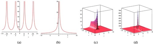
A graphical description is an essential tool for analysis and to communicate the answers to the problems lucidly. When working the calculation in daily life, we require the fundamental knowledge of securing the use of graphs. Hence, the graphical displays of some of the obtained solutions are demonstrated in Figures 1–6.

Figure 1. The $3D$ shape for $u_{12}$ under the constant values of $\lambda =3$, $\mu =1$, a = 0.1, b = 0.2, n = 2, $\alpha =0.35$, as well as t = 0.1 for the 2D shape. (a) Real $2D$ shape. (b) Imaginary $2D$ (c) shape Real $3D$ surface and Imaginary $3D$ surface.

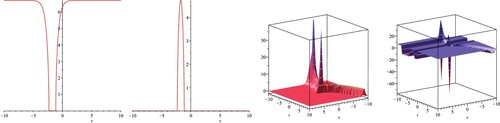
Figure 2. The $3D$ shape for $u_{14}$ under the constant values of $\lambda =2$, $\mu =2$, a = 0.1, b = 0.2, n = 2, $\alpha =0.35$, as well as t = 0.1 for the 2D shape. (a) Real $2D$ shape. (b) Imaginary $2D$ shape. (c) Real $3D$ surface and Imaginary $3D$ surface.

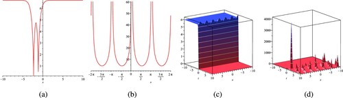
Figure 3. The $3D$ shape for $u_{22}$ under the constant values of $\lambda =3$, $\mu =1$, a = 0.1, b = 0.2, n = 2, $\alpha =0.35$ as well as t = 0.1 for the 2D shape. (a) Real $2D$ shape. (b) Imaginary $2D$ shape. (c) Real $3D$ surface and (d) Imaginary $3D$ surface.

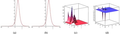
Figure 4. The $3D$ shape for $u_{23}$ under the constant values of $\lambda =2$, $\mu =2$, a = 0.1, b = 0.2, n = 2, $\alpha =0.35$ as well as t = 0.1 for the 2D shape. (a) Real $2D$ shape. (b) Imaginary $2D$ shape. (c) Real $3D$ surface and (d) Imaginary $3D$ surface.

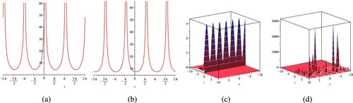
Figure 5. The $3D$ shape for $u_{32}$ under the constant values of $\lambda =3$, $\mu =1$, a = 0.1, b = 0.2, n = 2, $\alpha =0.35$ as well as t = 0.1 for the 2D shape. (a) Real $2D$ shape. (b) Imaginary $2D$ shape. (c) Real $3D$ surface and (d) Imaginary $3D$ surface.

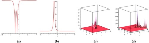
Figure 6. The $3D$ shape for $u_{35}$ under the constant values of $\lambda =2$, $\mu =1$, a = 0.1, b = 0.2, n = 2, $\alpha =0.35$ as well as t = 0.1 for the 2D shape. (a) Real $2D$ shape. (b) Imaginary $2D$ shape. (c) Real $3D$ surface and (d) Imaginary $3D$ surface.

4. Conclusions and future work

We have examined the modified $\left(G^{\prime }/G\right)$-expansion process for generating closed-form wave answers of the conformable fractional ZK equation, including power law nonlinearity. This scheme permits us to establish more many nonlinear conformable fractional evolution models in mathematical sciences by the examined models. As a consequence, various new types of closed-form wave answers are achieved. From our expert answers, we strongly conclude that the studied idea is great brawny, reliable, and crucial in executing numerous new closed-form wave answers of different nonlinear conformable FDEs. Finally, we mention that the process can be made to various distinct nonlinear conformable FDEs that occur in the area of mathematical physics.

Acknowledgments

The authors would like to acknowledge CAS-TWAS President's fellowship programme.

Disclosure statement

No potential conflict of interest was reported by the authors.

References

- Inc M, Yusuf A, Aliyu AI, et al. Time-fractional Cahn-Allen and time-fractional Klein-Gordon equations: lie symmetry analysis, explicit solutions and convergence analysis. Phys A Stat Mech Appl. 2018;493:94–106. doi: 10.1016/j.physa.2017.10.010
- Houwe A, Sabiu J, Hammouch Zet al,. Solitary pulses of the conformable derivative nonlinear differential equation governing wave propagation in low-pass electrical transmission line. Phys Scr 2019. in press. doi:10.1088/1402-4896/ab5055.
- Rawashdeh MS. A reliable method for the space-time fractional Burgers and time-fractional Cahn-Allen equations via the FRDTM. Adv Differ Equ. 2017;2017:1–14. doi: 10.1186/s13662-017-1148-8
- Hammouch Z, Mekkaoui ZT, Agarwal P. Optical solitons for the Calogero-Bogoyavlenskii-Schiff equation in (2+1)-dimensions with time-fractional conformable derivative. Eur Phys J Plus. 2018;248:133.
- Tariq H, Akram G. New approach for exact solutions of time fractional Cahn-Allen equation and time fractional Phi-4 equation. Physica A Stat Mech Appl. 2017;473(1):352–362. doi: 10.1016/j.physa.2016.12.081
- Mirzazadeh M, Alqahtani RT, Biswas A. Optical soliton perturbation with quadratic-cubic nonlinearity by riccati bernoulli sub-ODE method and Kudryashovs scheme. Optik. 2017;145:74–78. doi: 10.1016/j.ijleo.2017.07.011
- Alam MN, Alam MM. An analytical method for solving exact solutions of a nonlinear evolution equation describing the dynamics of ionic currents along microtubules. J Taibah Univ Sci. 2017;11:939–948. doi: 10.1016/j.jtusci.2016.11.004
- Alam MN, Belgacem FBM. Microtubules nonlinear models dynamics investigations through the exp−φ(ξ)-expansion method implementation. Mathematics. 2016;4:6. doi: 10.3390/math4010006
- Alam MN, Tunc C. An analytical method for solving exact solutions of the nonlinear Bogoyavlenskii equation and the nonlinear diffusive predator-prey system. Alex Eng J. 2016;55:1855–1865. doi: 10.1016/j.aej.2016.04.024
- Ekici M, Mirzazadeh M, Sonmezoglu A, et al. Optical solitons with anti-cubic nonlinearity by extended trial equation method. Optik. 2017;136:368–373. doi: 10.1016/j.ijleo.2017.02.004
- Younis M, Rehman HU, Rizvi STR, et al. Dark and singular optical solitons perturbation with fractional temporal evolution. Superlattices Microstruct. 2017;104:525–531. doi: 10.1016/j.spmi.2017.03.006
- Alam MN, Akbar MA, Hoque MF. Exact travelling wave solutions of the (3+1)-dimensional mKdV-ZK equation and the (1+1)-dimensional compound KdVB equation using new approach of the generalized (G′/G)-expansion method. Pramana J Phys. 2014;83(3):317–329. doi: 10.1007/s12043-014-0776-8
- Al-Shawbaa AA, Gepreel KA, Abdullaha FA, et al. Abundant closed form solutions of the conformable time fractional Sawada-Kotera-Ito equation using (G′/G)-expansion method. Results Phys. 2018;9:337–343. doi: 10.1016/j.rinp.2018.02.012
- Alam MN, Li X. Exact travelling wave solutions to higher order nonlinear equations. J Ocean Eng Sci. 2019;4(3):276–288. doi: 10.1016/j.joes.2019.05.003
- Alam MN. Exact solutions to the foam drainage equation by using the new generalized (G′/G)-expansion method. Results Phys. 2015;5:168–177. doi: 10.1016/j.rinp.2015.07.001
- Din STM, Bibi S. Exact solutions for nonlinear fractional differential equations using exponential rational function method. Opt Quant Electron. 2017;49:64. doi: 10.1007/s11082-017-0895-9
- Younis M. Optical solitons in (n+1)-dimensions with Kerr and power law nonlinearities. Modern Phys Lett B. 2017;31(15):1750186. doi: 10.1142/S021798491750186X
- Alam MN, Akbar MA, Mohyud-Din ST. A novel (G′/G)-expansion method and its application to the Boussinesq equation. Chin Phys B. 2014;23(2):020203. doi: 10.1088/1674-1056/23/2/020203
- Khan U, Ellahi R, Khan R, et al. Extracting new solitary wave solutions of Benny-Luke equation and Phi-4 equation of fractional order by using (G′/G)-expansion method. Opt Quant Electron. 2017;49:361. doi: 10.1007/s11082-017-1191-4
- Shallal MA, Jabbar HN, Ali KK. Analytic solution for the space-time fractional Klein-Gordon and coupled conformable Boussinesq equations. Results Phys. 2018;8:372–378. doi: 10.1016/j.rinp.2017.12.051
- Sahoo S, Ray SS. Solitary wave solutions for time fractional third order modified KdV equation using two reliable techniques (G′/G)-expansion method and improved (G′/G)-expansion method. Physica A. 2016;448:265–282. doi: 10.1016/j.physa.2015.12.072
- Unal E, Gokdogan A. Solution of conformable fractional ordinary differential equations via differential transform method. Optik-Int J Light Electron Opt. 2017;128:264–273. doi: 10.1016/j.ijleo.2016.10.031
- Wazwaz AM. Painlev analysis for a new integrable equation combining the modified Calogero-Bogoyavlenskii-Schiff (MCBS) equation with its negative-order form. Nonlinear Dyn. 2018;91:877–883. doi: 10.1007/s11071-017-3916-0
- Delgado VFM, Aguilar JFG, Torres L, et al. Exact solutions for the linard type model via fractional homotopy methods. Fract Deri Mittag-Leffler Kernel. 2019;194:269–291. doi: 10.1007/978-3-030-11662-0_16
- Saleh R, Mabrouk SM, Kassem M. Truncation method with point transformation for exact solution of Liouville Bratu Gelfand equation. Comput Math Appl. 2018;76:1219–1227. doi: 10.1016/j.camwa.2018.06.016
- Darvishi MT, Najafi M, Wazwaz AM. Soliton solutions for Boussinesq-like equations with spatio-temporal dispersion. Ocean Eng. 2017;130:228–240. doi: 10.1016/j.oceaneng.2016.11.052
- Martinez HY, Sosa IO, Reyes JM, et al. The Feng's first integral method applied to the nonlinear mKdV space-time fractional partial differential equation. Revista Mexicana de Fisica. 2016;62:310–316.
- Osman MS, Rezazadeh H, Eslami M. Traveling wave solutions for (3+1)-dimensional conformable fractional Zakharov-Kuznetsov equation with power law nonlinearity. Nonlinear Eng. 2019;8:559. doi: 10.1515/nleng-2018-0163
- Yaslan HC, Girgin A. New exact solutions for the conformable space-time fractional KdV, CDG, (2+1)-dimensional CBS and (2+1)-dimensional AKNS equations. J Taibah Univ Sci. 2019;13(1):1–8. doi: 10.1080/16583655.2018.1515303
- Saleh R, Kassem M, Mabrouk SM. Exact solutions of nonlinear fractional order partial differential equations via singular manifold method. Chinese J Phys. 2019;61:290–300. doi: 10.1016/j.cjph.2019.09.005
- Sabiu J, Jibril A, Gadu AM. New exact solution for the (3+1) conformable space–time fractional modified Korteweg–de-Vries equations via Sine-Cosine Method. J Taibah Univ Sci. 2019;13(1):91–95. doi: 10.1080/16583655.2018.1537642
- Tiwanaa MH, Maqbool K, Mann AB. Homotopy perturbation Laplace transform solution of fractional non-linear reaction diffusion system of Lotka-Volterra type differential equation. Eng Sci Tech. 2017;20(2):672–678.
- Mallaw F, Alzaidy JF, Hafez RM. Application of a Legendre collocation method to the space–time variable fractional-order advection–dispersion equation. J Taibah Univ Sci. 2019;13(1):324–330. doi: 10.1080/16583655.2019.1576265
- Pakchin SI, Javidi M, Kheiri H. Analytical solutions for the fractional nonlinear cable equation using a modified homotopy perturbation and separation of variables methods. Comput Math Math Phys. 2016;56(1):116–131. doi: 10.1134/S0965542516010103
- Ahmed HF. A numerical technique for solving multi-dimensional fractional optimal control problems. J Taibah Univ Sci. 2018;12(5):494–505. doi: 10.1080/16583655.2018.1491690
- Baskonus HM, Bulut H. On the numerical solutions of some fractional ordinary differential equations by fractional Adams-Bashforth-Moulton method. Open Math. 2015;13:547–556. doi: 10.1515/math-2015-0052
- Khan H, Arif M, Mohyud-Din ST, et al. Numerical solutions to systems of fractional Voltera Integro differential equations, using Chebyshev wavelet method. J Taibah Univ Sci. 2018;12(5):584–591. doi: 10.1080/16583655.2018.1510149
- Batista M. A closed-form solution for Reissner planar finite-strain beam using Jacobi elliptic functions. Int J Solids Struct. 2016;87:153–166. doi: 10.1016/j.ijsolstr.2016.02.020
- Nuruddeen RI, Nass AM. Exact solitary wave solution for the fractional and classical GEW-Burgers equations: an application of Kudryashov method. J Taibah Univ Sci. 2018;12(3):309–314. doi: 10.1080/16583655.2018.1469283
- Rahmatullah, Ellahi R, Din STMet al,. Exact traveling wave solutions of fractional order Boussinesq-like equations by applying exp-function method. Results Phys. 2018;8:114–120. doi: 10.1016/j.rinp.2017.11.023
- Martineza HY, Aguilarb JFG, Baleanu D. Beta-derivative and sub-equation method applied to the optical solitons in medium with parabolic law nonlinearity and higher order dispersion. Optik. 2018;155:357–365. doi: 10.1016/j.ijleo.2017.10.104
- Sohail A, Maqbool K, Ellahi R. Stability analysis for fractional-order partial differential equations by means of space spectral time Adams-Bashforth Moulton method. Num Meth Partial Differ Equ. 2018;34(1):19–29. doi: 10.1002/num.22171
- Rahmatullah ER, Mohyud-Din ST, Khan U. Exact traveling wave solutions of fractional order Boussinesq-like equations by applying Exp-function method. Results Phys. 2018;8:114–120. doi: 10.1016/j.rinp.2017.11.023
- Sohail A, Wajid HA, Rashidi MM. Numerical modeling of capillary-gravity waves using the phase field method. Surf Rev Lett. 2014;21(03):1450036. doi: 10.1142/S0218625X1450036X
- Arshad S, Siddiqui AM, Sohail A, et al. Comparison of optimal homotopy analysis method and fractional homotopy analysis transform method for the dynamical analysis of fractional order optical solitons. Adv Mech Eng. 2017;9(3):1–12. doi: 10.1177/1687814017692946
- Matebese BT, Adem AR, Khalique CM, et al. Solutions of Zakharov-Kuznetsov equation with power law nonlinearity in (1+3)-dimensions. Phys Wave Phenomena. 2011;19(2):148–154. doi: 10.3103/S1541308X11020117
- Zhou DZ, Yong C, Huai LY. Symmetry reduction and exact solutions of the (3+1)-dimensional Zakharov-Kuznetsov equation. Chinese Phys B. 2010;19(9):090205.
- Khalil R, AlHorani M, Yousef A, et al. A new definition of fractional derivative. J Comput Appl Math. 2014;264:65–70. doi: 10.1016/j.cam.2014.01.002
- Atangana A, Baleanu D, Alsaed A. New properties of conformable derivative. Open Math. 2015;13:889–98. doi: 10.1515/math-2015-0081
- Abdeljawad T. On conformable fractional calculus. J Comput Appl Math. 2015;279:57–66. doi: 10.1016/j.cam.2014.10.016
- Shahid N, Tunc C. Resolution of coincident factors in altering the flow dynamics of an MHD elastoviscous fluid past an unbounded upright channel. J Taibah Univ Sci. 2019;13(1):1022–1034. doi: 10.1080/16583655.2019.1678897
- Golmankhaneh AK. A review on application of the local fractal calculus. Num Com Meth Sci Eng. 2019;1(2):57–66.
- Golmankhaneh AK, Fernandez A. Random variables and stable distributions on fractal cantor sets. Fractal Fractional. 2019;3(2):31. doi: 10.3390/fractalfract3020031
- Golmankhaneh AK, Tunc C. Stochastic differential equations on fractal sets. Stochastics. 2019. doi:10.1080/17442508.2019.1697268.
- Hameed M, Khan AA, Ellahi R, et al. Study of magnetic and heat transfer on the peristaltic transport of a fractional second grade fluid in a vertical tube. Eng Sci Tech. 2015;18(3):496–502.
- Ma X, Pan Y, Chang L. Explicit travelling wave solutions in a magneto-electro-elastic circular rod. Inter J Comput Sci. 2013;10(1):62–68.
- Tunç C, Tunç O. Qualitative analysis for a variable delay system of differential equations of second order. J Taibah Univ Sci. 2019;13(1):468–477. doi: 10.1080/16583655.2019.1595359