Bifurcation and travelling wave solutions for a (2+1)-dimensional KdV equation

Abstract

This work aims to study a new $\left(2+1\right)KdV$ equation that is recently introduced in (Phys. Lett. A. 383: 728–731, 2019). By using the method of dynamical systems, we examine the bifurcation and construct exact travelling wave solutions for a (2+1) KdV equation. Exact parametric representations of all wave solutions are introduced and they are clarified graphically.

KEYWORDS:

• Travel wave solution
• bifurcation
• phase portrait
• $\left(2+1\right)KdV$ equation

1. Introduction

The construction of the new travelling wave solutions for nonlinear evolution equations (NELLEs) is substantial and significant in various sides for the majority of phenomena physical and mathematics. The nonlinear wave phenomena arise in numerous branches of engineering and science, such as ocean engineering fluid mechanics, chemical kinematics, biology, solid-state physics, chemical physics, geochemistry, and meteorology [1–4]. The nonlinear wave phenomena of dissipation, reaction, diffusion, dispersion and convection are very meaningful in nonlinear wave equations. Thus, the search for the exact solutions for those equations has long been one of the fundamental topics of the perennial interest in mathematics and physics. In the procedures of seeking for exact solutions for those equations, numerous methods have been introduced and some of them have been developed, such as homogeneous balance method [5], Darboux transformations [6,7], extended tanh method [8,9], inverse scattering transform [10] and so on. It is well known that the traditional $\left(1+1\right)KdV$ equation (1) $u_t+6u{u}_x+u_{xxx}=0$(1) is a famous one that is utilized to characterize the waves on shallow water surfaces. Several authors have studied numerous versions of the $KdV$ equation with distinct procedures and techniques from diverse points of view (see, e.g. [11–18]) and the references therein.

Recently in 2019, a new (2+1)-dimensional KdV equation has been proved based on the extended Lax pair and has been announced in [19]. It takes the following form: (2) $\begin{array}{r}{u}_t+6u^2\left(u_y-u_x\right)-u_{xxx}+u_{yy}+3u_{xxy}-3u_{xyy}=0.\end{array}$(2)

To our knowledge, Equation (2) was not previously studied in other works from the point of view of constructing the travelling wave solutions, which may be helpful in understanding the physical interpretation for it. This motivates us to utilize the combination of the qualitative theory for differential equation and bifurcation for planar dynamical system associated with Equation (2) to construct new exact travelling wave solutions based on different values of the parameters.

Notice that, if $u$ does not depend on $x$ independently, i.e. $u=u\left(y,t\right)$, Equation (2) reduces immediately (3) $u_t+6u^2{u}_y+u_{yyy}=0.$(3)

Re-expressing the variable $y$ as $x$ we get the traditional $mKdV$ equation.

This paper is organized as follows: Section two contains a popular transformation which is utilized to convert the given time-evolution Equation (2) a planar conservative Hamiltonian system. Section three, we study the phase portrait for the deduced planar system in section two. In section four, based on the formula of the total energy corresponding to the deduced planar system, we construct several types of travelling wave solution and illustrate them graphically.

2. Travelling wave transformation

In this subsection, we apply the transformation: (4) $u\left(x,y,t\right)=u\left(\xi \right),\xi =k_{1}x+k_{2}y+ct,$(4) to Equation (2) to be able to construct a travelling wave solution, we obtain (5) $c{u}^{\mathrm{\prime }}+3\lambda u^2{u}^{\mathrm{\prime }}+\overline{\lambda }{u}^{\mathrm{\prime }\mathrm{\prime }\mathrm{\prime }}=0$(5) where ′ denotes derivatives with respect to $\xi$ while (6) $\lambda =2\left(k_2-k_1\right),\overline{\lambda }=\left(k_2-k_1\right)\left(k_2^2+4k_1{k}_2+k_1^2\right),$(6) where $k_1$ and $k_2$ are arbitrary constants and $c$ is the speed of the wave. Integrating Equation (5) with respect to $\xi$ and equating the integration constant to zero, we obtain (7) $u^{\mathrm{\prime }\mathrm{\prime }}=\frac{-cu-\lambda u^3}{\overline{\lambda }}$(7) Equation (7) can be expressed as a system of first-order differential equations in the following form (8) $u^{\mathrm{\prime }}=z,z^{\mathrm{\prime }}=\frac{-cu-\lambda u^3}{\overline{\lambda }}$(8) Preforming the transformation (9) $d\xi =\overline{\lambda }d\tau ,$(9) to the dynamical system (8), we obtain (10) $\frac{du}{d\tau }=\overline{\lambda }z,\frac{dz}{d\tau }=-\left(cu+\lambda u^3\right)$(10) It is worth noting that the dynamical system (10) is a conservative Hamiltonian system that describes physically the motion of a particle in the Euclidean plane under the influence of the potential forces. The Hamiltonian function (Total energy) takes the following form (11) $H=\frac{1}{2}\overline{\lambda }{z}^2+\frac{c}{2}{u}^2+\frac{\lambda }{4}{u}^4=h,$(11) where $h$ is an arbitrary constant denoting the value of the energy. The Hamiltonian system (10) is one-dimensional integrable system. Thus, the constant of motion, the total energy, is given by (11) and is used to find the explicit solution of the Hamiltonian system (10) and so, we can construct a travelling wave solution for Equation (2). For more details about the integrable systems with more than one dimension (see, e.g. [20–23]).

3. Bifurcation and phase portrait of Equation (2)

In this section, we are interested in investigating all the possible bifurcations and phase portrait for the dynamical system (10), taking into account the transformation (9). It is clear that the equilibrium points corresponding the Hamiltonian system (10) laying on the axis $z=0$ are the zeros of $f\left(u\right)=cu+\lambda u^2.$ Thus, the Hamiltonian system (10) has $E_1=\left(0,0\right)$ as a unique equilibrium point if $c\lambda \ge 0$, while if $c\lambda <0$, it has three equilibrium points that are $E_1=\left(0,0\right)$ and $E_{2,3}=\left(\pm \sqrt{(-c/\lambda )},0\right)$. The determinant of the Jacobi matrix corresponding to the Hamiltonian system (10) admits the following form (12) $det\left[J\left(u_0,0\right)\right]=\overline{\lambda }\left[c+3\lambda u_0^2\right],$(12) where $\left(u_0,0\right)$ is any equilibrium point for the system (10). According to the theory of planar dynamical system, the equilibrium point $\left(u_0,0\right)$ of the planar integrable dynamical system (10) is either saddle point if $det\left[J\left(u_0,0\right)\right]<0$ or centre point if $det\left[J\left(u_0,0\right)\right]>0$ or cusp point if $det\left[J\left(u_0,0\right)\right]=0$ besides the poincare index of this equilibrium point is zero. The values of the energy $h$ at those equilibrium points are (13) $h_1=H\left(0,0\right)=0,h_2=H\left(\pm \sqrt{\frac{-c}{\lambda }},0\right)=\frac{-c2}{4\lambda }$(13) The determinants of the Jacobi matrix (12) calculated at the equilibrium points $Ei,i=1,2,3$ are (14) $\begin{array}{rl}\text{det}\left[J\left(E_1\right)\right]& =c\overline{\lambda },\end{array}$(14) (15) $\begin{array}{rl}\text{det}\left[J\left(E_{2,3}\right)\right]& =-2c\overline{\lambda }\end{array}$(15) We have three bifurcation curves: (16) $L_1:\overline{\lambda }=0,L_2:c=0,L_3:\lambda =0,$(16) Those curves divide the space of the parameters into 10 regions that are defined as $\begin{array}{rl}{R}_1& =\left\{\right(\overline{\lambda },c,\lambda )|\overline{\lambda }>0,c<0,\lambda <0\},\end{array}$ $\begin{array}{rl}{R}_2& =\left\{(\overline{\lambda },c,\lambda )|\overline{\lambda }<0,c>0,\lambda >0\right\},\end{array}$ $\begin{array}{rl}{R}_3& =\left\{\right(\overline{\lambda },c,\lambda )|\overline{\lambda }>0,c>0,\lambda >0\},\end{array}$ $\begin{array}{rl}{R}_4& =\left\{\right(\overline{\lambda },c,\lambda )|\overline{\lambda }<0,c<0,\lambda <0\},\end{array}$ $\begin{array}{rl}{R}_5& =\left\{\right(\overline{\lambda },c,\lambda )|\overline{\lambda }>0,c=0,\lambda >0\},\end{array}$ $\begin{array}{rl}{R}_6& =\left\{\right(\overline{\lambda },c,\lambda )|\overline{\lambda }<0,c=0,\lambda <0\},\end{array}$ $\begin{array}{rl}{R}_7& =\left\{\right(\overline{\lambda },c,\lambda )|\overline{\lambda }>0,c>0,\lambda <0\},\end{array}$ $\begin{array}{rl}{R}_8& =\left\{\left(\overline{\lambda },c,\lambda \right)|\overline{\lambda }>0,c<0,\lambda >0\right\},\end{array}$ $\begin{array}{rl}{R}_9& =\left\{\right(\overline{\lambda },c,\lambda )|\overline{\lambda }<0,c>0,\lambda <0\},\end{array}$ (17) $\begin{array}{rl}{R}_{10}& =\left\{\left(\overline{\lambda },c,\lambda \right)|\overline{\lambda }<0,c<0,\lambda >0\right\}.\end{array}$(17)

Taking into account the above restriction on the parameters and utilizing the software Maple for symbolic computations, we can present the phase portrait for the system (10) in the plane $\left(u,z\right).$

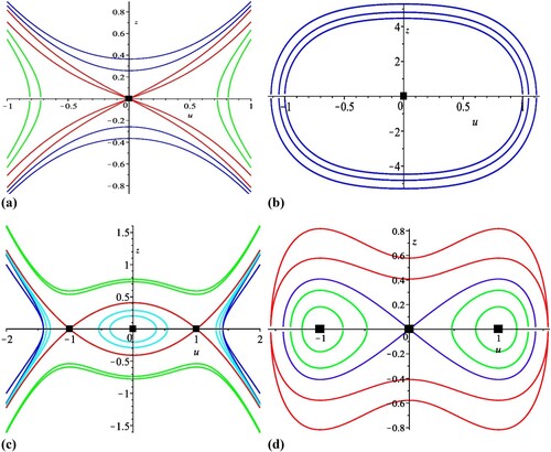
Case I: When $\left(\overline{\lambda },c,\lambda \right)\in R_1$, the dynamical system (10) has a unique equilibrium point $E_1=\left(0,0\right)$ and it is a saddle point because the determinant of the Jacobi matrix (14) is negative. The phase portrait for this case is clarified in Figure 1(a).

Figure 1. The level curves defined by $H\left(u,\frac{du}{d\xi }\right)=h$ for different values of $h$ and the parameters $c,\lambda ,\overline{\lambda }.$ The solid black box indicates the equilibrium points.

Case II: When $\left(\overline{\lambda },c,\lambda \right)\in R_2$, $E_1=\left(0,0\right)$ is a unique equilibrium point, and the determinant of the Jacobi matrix (14) is negative , so it is a saddle point. The phase portrait for this case is outlined in Figure 1(a).

Case III: When $\left(\overline{\lambda },c,\lambda \right)\in R_3$, the point, $E_1=\left(0,0\right)$ is a unique equilibrium point for a system (10). It is a centre since the determinant of the Jacobi matrix (14) is positive. The phase portrait for this case is illustrated in Figure 1(b).

Case IV: When $\left(\overline{\lambda },c,\lambda \right)\in R_4$, the equilibrium point $E_1$ is unique and it is a centre since the determinant of the Jacobi matrix (14) is positive. The phase portrait for this case is outlined in Figure 1(b)

Case V: Assuming $\left(\overline{\lambda },c,\lambda \right)\in R_5$, the system (10) has a unique equilibrium point $E_1=\left(0,0\right)$ which is a centre point. The phase portrait for this case is clarified in Figure 1(b)

Case VI: For$\left(\overline{\lambda },c,\lambda \right)\in R_6$, the dynamical system (10) has a unique equilibrium point $E_1=\left(0,0\right)$ that is a saddle point. The phase portrait for the present case is outlined in Figure 1(a).

Case VII: For $\left(\overline{\lambda },c,\lambda \right)\in R_7$, the dynamical system (10) has three equilibrium points $E_1$ and $E_{2,3}$. As a result of that, the determinant of the Jacobi matrix (14) is positive, $E_1$ it is a centre point. While the determinant of the Jacobi matrix (15) is negative, the equilibrium points $E_{2,3}$ are saddle points. The phase portrait is clarified in Figure 1(c).

Case VIII: If $\left(\overline{\lambda },c,\lambda \right)\in R_8$, the dynamical system (10) has three equilibrium points $E_1$ and $E_{2,3}$. The equilibrium point $E_1$ is a saddle point, while the other two are centres as it is outlined in Figure 1(d).

Case IX: When $\left(\overline{\lambda },c,\lambda \right)\in R_9$ the dynamical system has three equilibrium points $E_1$ is a saddle point due to the determinant of the Jacobi matrix (14) is negative, while the other two are centre points as a result of that, the determinant of the Jacobi matrix (15) is positive Figure 1(d).

Case X: If $\left(\overline{\lambda },c,\lambda \right)\in R_{10}$, the dynamical system (10) has three equilibrium points, $E_1$ and $E_{2,3}$ and is a center point, while the other two equilibrium points are saddle points. The phase portrait for this case is outlined in Figure 1(c).

Remark 1: We notice that there is more than a case can be described by the same figure that represents the phase portrait. These figures are not completely identical. Let us clarify that: For the case VII, the green colour curves define orbits in the phase space for the dynamical system (10) on a certain level of the energy $h>(-c2/4\lambda )$, while the similar curve in case X represents the orbits for the dynamical system (10) on the level $h<(-c2/4\lambda )$ of the energy. The red colour curves represent the orbits in the phase space for the system (10) on a zero level of the energy for both cases. For case VII, the blue curves represent the orbits in the phase space for the system (10) on a zero level of the energy, but similar curves represent the orbits of the system (10) on a level $h>(-c2/4\lambda )$ of the energy for case X. Similar conclusion can be done for the other figures. Moreover, this will be illustrated in more detail in the following section.

4. Exact travelling wave solution

Assume that $u\left(\xi \right)$ is a continuous solution for the $\left(2+1\right)KdV$ equation for $\xi \in R$ and$\underset{\xi \to \mathrm{\infty }}{lim}u\left(\xi \right)=l_1,\underset{\xi \to \mathrm{\infty }}{lim}u\left(\xi \right)=l_2.$ When $l_1=l_2$, the solution $u\left(\xi \right)$ is named a solitary wave solution, and otherwise, it is called a kink (or anti-kink) wave solution. It is well known that homoclinic, heteroclinic and periodic orbits of the dynamical system (10) correspond to solitary, kink (or anti-kink) and periodic wave solutions, respectively. Therefore to examine all the bifurcations of solitary waves, kink waves and periodic waves for Equation (2), we must find all periodic annuli of the dynamical system (10) depending on the parameter space. The exact parametric representation for all bounded functions $u\left(\xi \right)$ is equivalent to construct exact travelling wave solutions for Equation (2). We utilize the energy integral (11) to find such solutions. It gives (18) $\int \frac{du}{\sqrt{P_4\left(u\right)}}=\sqrt{\frac{2}{\overline{\lambda }}}\int d\xi ,$(18) where $P_4\left(u\right)$ is a polynomial of degree four in $u$ and it takes the following form (19) $P_4\left(u\right)=h-\frac{c}{2}{u}^2-\frac{\lambda }{4}{u}^4.$(19) Depending on the values of $c,\overline{\lambda },\lambda$ and on a certain level of energy $h$, we can evaluate the integral in Equation (18) and construct a travelling wave solution for Equation (2).

4.1. Suppose ($\overline{\lambda },c,\lambda )\in R_1$

As it is outlined in Figure 1(a), there are three families of orbits for different values of the parameters $h$. The explicit representation for the travelling wave solution of Equation (2) is introduced by using Equation (18) for different values of the parameter $h$:

• On a zero-level of the total energy (11), a family of orbits pass through the origin. This family appears with a red colour in Figure 1(a). Thus, the polynomial (19) is $P_4\left(u\right)=\frac{-\lambda }{4}{u}^2\left[\frac{2c}{\lambda }+u^2\right].$ The expression (18) gives (20) $u\left(\xi \right)=-\sqrt{\frac{2c}{\lambda }}\text{csch}\sqrt{\frac{-c}{\lambda }}\left(\xi +\delta \right),$(20)

where $\delta$ is an arbitrary integration constant. The solution (20) is clarified in Figure 2(a).

• On a positive level of the energy h > 0, there is a family of orbits with blue colour as it is outlined in Figure 1(a). These orbits do not intersect the $u$-axis ($z=0$) and so the polynomial (19) does not have real zeroes, i.e. $P_4\left(u\right)=-\frac{\lambda }{4}\left(u_1^2+u^2\right)\left(u_2^2+u^2\right).$ The expression (18) gives (21) $u\left(\xi \right)=-u_1\frac{\text{sn}\left[u_2\sqrt{\frac{-\lambda }{2\overline{\lambda }}}\left(\xi +\delta \right),\sqrt{1-\frac{u_1^2}{u_2^2}}\right]}{\text{cn}\left[u_2\sqrt{\frac{-\lambda }{2\overline{\lambda }}}\left(\xi +\delta \right),\sqrt{1-\frac{u_1^2}{u_2^2}}\right]},$(21) where $\text{sn}\left(u,k\right),\text{cn}\left(u,k\right)$ and $\text{dn}\left(u,k\right)$ are the Jacobi elliptic functions [24]. The travelling wave solution (21) is illustrated in Figure 2(b).

• On a negative level of the energy, the Hamiltonian system (10) has a family of orbits with green colour as it is clarified in Figure 1(a). These orbits intersect the u-axis in two points, so the polynomial (19) has two real zeroes, i.e. $P_4\left(u\right)=-\frac{\lambda }{4}\left(u^2-u_1^2\right)\left(u^2+u_2^2\right).$ The expression (18) implies the following. (22) $u\left(\xi \right)=\frac{\text{cn}\left[\sqrt{\frac{-\lambda }{2\overline{\lambda }}\left(u_1^2+u_2^2\right)}\left(\xi +\delta \right),\frac{u_2}{\sqrt{u_1^2+u_2^2}}\right]}{\text{d}{\text{n}}^2\left[\sqrt{\frac{-\lambda }{2\overline{\lambda }}\left(u_1^2+u_2^2\right)}\left(\xi +\delta \right),\frac{u_2}{\sqrt{u_1^2+u_2^2}}\right]}.$(22)

Figure 2. The profile of the travelling wave solutions for different values of the parameters.

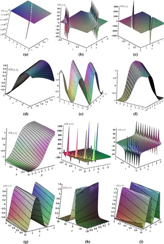
The travelling wave solution (22) is illustrated in Figure 2(c).

4.2 . Suppose $\left(\overline{\lambda },c,\lambda \right)\in R_2$

There are three families of orbits for the Hamiltonian system (10). These families are defined by $H\left(u,z\right)=h$ for different values of $h$. In Figure 1(a), the family of orbits with red colour is defined on a zero level of the constant $h$ see, Figure 1(a) and the parametric representation of the travelling wave solution is given by equation (20) and it is clarified in Figure 2(a). On a negative level of h, the orbits with blue colour are defined by $H\left(u,z\right)=h\in \left]-\mathrm{\infty },0\right[$, see, Figure 1(b). The parametric representation of the travelling wave solution is obtained by Equation (21) and it is outlined in Figure 2(b). The orbits with green colour correspond to $H\left(u,z\right)=h$, where $h>0$, see, Figure 1(a). The parametric representation of the travelling wave solution reads as Equation (22) and it is illustrated by Figure 2(c).

4.3. Suppose $\left(\overline{\lambda },c,\lambda \right)\in R_3$

There are a family of periodic orbits around the origin that is defined by $H\left(u,z\right)=h$, where as it is outlined in Figure 1(b). The existence of this type of orbits refers to the existence of periodic travelling wave solutions. Any orbit of this family intersects the u-axis ($z=0$), i.e. the polynomial (19) has two real zeroes and so $P_4\left(u\right)=\frac{\lambda }{4}\left(u_1^2-u^2\right)\left(u_2^2+u^2\right),$where $u_2^2>u_1^2.$ Consequently, the expression (18) leads to (23) $\begin{array}{rl}u\left(\xi \right)& =\frac{u_2}{\sqrt{u_1^2+u_2^2}}\\ & \times \frac{\text{cn}\left[\sqrt{\frac{-\lambda }{2\overline{\lambda }}\left(u_1^2+u_2^2\right)}\left(\xi +\delta \right),\frac{-u_2}{\sqrt{u_1^2+u_2^2}}\right]}{\text{d}{\text{n}}^2\left[\sqrt{\frac{-\lambda }{2\overline{\lambda }}\left(u_1^2+u_2^2\right)}\left(\xi +\delta \right),\frac{-u_2}{\sqrt{u_1^2+u_2^2}}\right]}.\end{array}$(23)

It is clear that the travelling wave solution (23) is periodic with period (24) $4\sqrt{\frac{2\overline{\lambda }}{\lambda \left(u_1^2+u_2^2\right)}}K\left(\frac{-u_1}{\sqrt{u_1^2+u_2^2}}\right),$(24) where $K\left(k\right)$ is a complete elliptic integral of the first type. Figure 2(d) illustrates the solution (23).

4.4. Suppose $\left(\overline{\lambda },c,\lambda \right)\in R_4$

This case is similar to the previous case. The explicit representation of the travelling wave solution is given by (23) and it is clarified by Figure 2(d).

4.5. Suppose $\left(\overline{\lambda },c,\lambda \right)\in R_5$

There is a family of periodic orbits around the origin as it is outlined in Figure 1(b). This family corresponds to the curves defined by $H\left(u,z\right)=h$, where $h>0$. Following Figure 1(b), any orbit of this family intersects the u-axis ($z=0$) in two points, so the polynomial $P_4\left(u\right)$ has two real zeroes, i.e. $P_4\left(u\right)=\frac{\lambda }{4}\left(u_1^2-u^2\right)\left(u_2^2+u^2\right),$where $u_1^2=\sqrt{\frac{4h}{\lambda }}.$ Consequently, the expression (18) leads to (25) $u\left(\xi \right)=\frac{u_1}{\sqrt{2}}sn\left[u_1\sqrt{\frac{\lambda }{2\overline{\lambda }}}\left(\xi +\delta \right),-\frac{1}{\sqrt{2}}\right].$(25) Notice that the solution (25) does not contain t explicitly due to $c=0$ in the region $R_5$. This type of solution is named static solution and it is is clarified by Figure 2(e).

4.6. Suppose $\left(\overline{\lambda },c,\lambda \right)\in R_6$

There is a family of orbits as outlined in Figure 1(a) with green colour. This family is defined by $H\left(u,z\right)=h$, where $h<0$. For this case, any orbit of this family intersects the u-axis ($z=0$) in two points and having a green colour as outlined in Figure 1(a). Thus, the polynomial (19) has two real zeroes and it takes the following form $P_4\left(u\right)=-\frac{\lambda }{4}\left(u^2-u_1^2\right)\left(u^2+u_1^2\right).$The expression (18) implies to (26) $u\left(\xi \right)=\frac{\text{cn}\left[\sqrt{\frac{\lambda }{2\overline{\lambda }}}\left(\xi +\delta \right),\frac{1}{\sqrt{2}}\right]}{\text{d}{\text{n}}^2\left[\sqrt{\frac{\lambda }{2\overline{\lambda }}}\left(\xi +\delta \right),\frac{1}{\sqrt{2}}\right]}.$(26)

The solution (26) represents a static solution for Equation (2). Figure 2(f) illustrates solution (26).

4.7. Suppose $\left(\overline{\lambda },c,\lambda \right)\in R_7$

For this case, there are four families of orbits that are defined by the curves $H\left(u,z\right)=h$, where $h$ is either $h=-\frac{c^2}{4\lambda }$ or $h=0$ or $h>-\frac{c^2}{4\lambda }$ or $0<h<-\frac{c^2}{4\lambda }$, as outlined by Figure 1(c). Let us study each case individually:

• When $h=-\frac{c^2}{4\lambda },$ there is a family of orbits connecting the two saddle points and they are defined by $H\left(u,z\right)=-\frac{c^2}{4\lambda }.$ These orbits are characterized by red colour as it is outlined by Figure 1(c). Any orbits of this family intersect the u-axis $\left(z=0\right)$ in two points that are saddle points, so the polynomial (19) has two repeated real zeroes and it takes the following form $P_4\left(u\right)=-\frac{\lambda }{4}{\left(u^2+\frac{c}{\lambda }\right)}^2.$ Thanks to the expression (18), we get the explicit representation of the travelling wave solution in the following form (27) $u\left(\xi \right)=\sqrt{\frac{-\lambda }{c}}\text{tanh}\sqrt{\frac{c}{2\overline{\lambda }}}\left(\xi +\delta \right).$(27)

Figure 2(g) illustrates the travelling wave solution (27).

• When $h=0$, there is a family of orbits that are outlined in Figure 1(c) with a blue colour. Any orbit of this family does not intersect the $z$axis ($u=0$). The polynomial (19) reads as $P_4\left(u\right)=-\frac{\lambda }{4}{u}^2\left(u^2+\frac{2c}{\lambda }\right)$ and under the expression (18), the travelling wave solution for equation (2) admits the following form (28) $u\left(\xi \right)=\sqrt{\frac{-2c}{\lambda }}\text{sec}\sqrt{\frac{c}{\overline{\lambda }}}\left(\xi +\delta \right).$(28)

Figure 2(h) clarifies the solution (28).

• On the level, $h>-\frac{c^2}{4\lambda },$ there is a family of orbits having a green colour in Figure 1(c). These orbits do not intersect the u-axis ($z=0)$ and the polynomial (19) has complex roots. The polynomial (19) has the form $P_4\left(u\right)=-\frac{\lambda }{4}\left(u^2+u_1^2\right)\left(u^2+u_2^2\right),$ where $u_{1,2}^2=a+ib.$ Using the expression (18), we obtain a travelling wave solution in the form (29) $\begin{array}{rl}u\left(\xi \right)& =\sqrt{\frac{a^2+b^2}{ib-a}}sn\\ & \times \left[\sqrt{\frac{\lambda \left(a-ib\right)}{2\overline{\lambda }}}\left(\xi +\delta \right),\frac{a+ib}{\sqrt{a^2+b^2}}\right].\end{array}$(29)

The solution (29) is illustrated in Figure 2(i).

• On the level, $0<h<-\frac{c^2}{4\lambda },$ there is a family of periodic orbits around the origin. This family is characterized by $H\left(u,z\right)=h$ and it is outlined by cyan colour in Figure 1(c). Any orbit of this family cuts the u-axis ($z=0$) in four points and so the polynomial (18) has four real zeroes and so it becomes $P_4\left(u\right)=-\frac{\lambda }{4}\left(u^2-u_1^2\right)\left(u^2-u_2^2\right)$. The expression (18) gives an explicit travelling wave solution for Equation (2) in the following form (30) $u\left(\xi \right)=u_{2}sn\left[\sqrt{\frac{-\lambda }{2\overline{\lambda }}}\left(\xi +\delta \right),\frac{u_2}{u_1}\right].$(30)

Figure 2(j) clarifies solution (30).

4.8. Suppose $\left(\overline{\lambda },c,\lambda \right)\in R_8$

For this case there are different families of orbits for the Hamiltonian system (10) and these orbits are defined by $H\left(u,z\right)=h$ for different values of the constant $h$, where $h>0,$ $h=0$, $h\in \left]\frac{-c^2}{4\lambda },0\right[.$ Let us study and examine each case individually:

• On the level h > 0, there is a family of orbits which intersect the u-axis ($z=0$) in two points, as outlined by red colour in Figure 1(d). Thus, the polynomial (19) has two real zeroes, so it becomes $P_4\left(u\right)=\frac{\lambda }{4}\left(u_1^2-u^2\right)\left(u_2^2+u^2\right).$ By virtue of expression (18), we can construct a travelling wave solution for Equation (2) as given by Equation (23) and it is outlined by Figure 2(d).

• On a zero level of the energy, there is an orbit passing through the origin which is a saddle point and returns to it again, as illustrated by blue curves in Figure 1(d). This type of orbits is named homoclinic orbit, which refers usually to the existence of solitary wave solution. It is clear from Figure 1(d), such orbit intersects the u-axis ($z=0$) in three points and so, the polynomial (19) becomes $P_4\left(u\right)=\frac{\lambda }{4}{u}^2\left[-\frac{2c}{\lambda }-u^2\right].$ Thanks the expression (18), we obtain (31) $u\left(\xi \right)=\sqrt{\frac{-2c}{\lambda }}\text{sech}\sqrt{\frac{-c}{\lambda }}\left(\xi +\delta \right).$(31)

Solution (31) is clarified by Figure 2(k).

• For $h\in \left]\frac{-c^2}{4\lambda },0\right[,$ equation $H\left(u,z\right)=h$ defines periodic orbits around the two equilibrium points $E_{2,3}$. Any orbit of this family intersects the $u-$ axis ($z=0$) in four points, so the polynomial (19) has four real zeroes, so it can be written as $P_4\left(u\right)=\frac{\lambda }{4}\left(u_1^2-u^2\right)\left(u_2^2-u^2\right).$ The periodic travelling wave solution for this case can be obtained from Equation (30) by replacing $\lambda$ by $-\lambda$ and it is illustrated by Figure 2(j).

4.9. Suppose $\left(\overline{\lambda },c,\lambda \right)\in R_9$

There are different families of orbits for the Hamiltonian system (10) that are defined by $H\left(u,z\right)=h$ different values of the constant $h:h<0,h=0,h\in \left]0,\frac{-c^2}{4\lambda }\right[.$

They are outlined in Figure 1(d) in different colours. Let us study them individually.

• There is a family of periodic orbits around the equilibrium points. These orbits are defined by $H\left(uz\right)=h,$ where $h<0$, and they are clarified by red colour in Figure 1(d). Any orbit of this family intersects the u-axis ($z=0$) in two points. This clarifies the polynomial (18) has two real zeroes, so it reads as $P_4\left(u\right)=-\frac{\lambda }{4}\left(u^2-u_1^2\right)\left(u^2+u_2^2\right).$ Thanks to expression (18), the travelling wave solution for Equation (2) can be obtained from Equation (22) by replacing $u_2$ by $u_1$. This solution is illustrated in Figure 2(c).

• On a zero level of the energy h, there is a heteroclinic orbit that is defined by $H\left(u,z\right)=0$ and it is outlined by blue colour in Figure 1(d). The travelling wave solution for Equation (2) is given by Equation (28) and it is illustrated by Figure 2(h).

• Equation $H\left(u,z\right)=h,$ where $h\in \left]0,-\frac{c^2}{4\lambda }\right[$ defines two families of periodic orbits around the two centre points $E_{2,3}$ and they are illustrated by Figure 1(d) by green colour. Figure 1(d) illustrates that the polynomial (19) has four real zeroes, so it can be rewritten as $P_4\left(u\right)=\frac{\lambda }{4}\left(u_1^2-u^2\right)\left(u^2-u_2^2\right).$ Using expression (18), the travelling wave solution for Equation (2) takes the following form (32) $u\left(\xi \right)=\frac{u_2}{\text{dn}\left[\sqrt{\frac{\lambda }{2\overline{\lambda }}}\left(\xi +\delta \right),\sqrt{1-\frac{u_2^2}{u_1^2}}\right]}.$(32)

Solution (32) is clarified by Figure 2(l).

4.10. Suppose $\left(\overline{\lambda },c,\lambda \right)\in R_{10}$

There are different families of orbits for the Hamiltonian system (10) and they are defined by $H\left(u,z\right)=h$ for different values of h as it is outlined in Figure 1(c) with different colours.

• On the level $h=-\frac{c^2}{4\lambda },$ the corresponding family of heteroclinic orbits is illustrated by Figure 1(c) with red colour. The travelling wave solution for equation (2) can be obtained by equation (27) and it is clarified by Figure 2(g).

• When $h>0$, the travelling wave solution for Equation (2) can be obtained by Equation (22) and it is illustrated in Figure 2(c).

• When $h\in \left]-\frac{c^2}{4\lambda },0\right[$ the travelling wave solution for Equation (2) is Equation (30) and it is clarified by Figure 2(j).

• When $h\in \left]-\mathrm{\infty },\frac{-c^2}{4\lambda }\right[$, Equation (2) has the travelling wave solution (21) and it is clarified by Figure 2(b).

Remark 2: PDE equation (2) is regarded as an extension or generalization of the mKdV equation. Consequently, we can construct some exact travelling wave solutions for the mKdV equation (3) as special cases from the new solutions of equation (2). Let us clarify that with some details. To construct a travelling wave solution for the mKdV equation (3), we consider the change of variables (4) with $k_1=0,k_2=1.$ Inserting those values in Equation (6), we get $\lambda =2$ and $\overline{\lambda }=1.$ Thus, we have (33) $\left(\overline{\lambda },c,\lambda \right)=\left(1,c,2\right)\in R_3\cup R_5\cup R_8.$(33) Based on the sign of the parameter $c$, we study the following three possible cases one by one:

Case (I): For $\left(1,c,2\right)\in R_3,$ the mKdV equation (3) has a periodic travelling wave solution in the form (23) with $u_1^2=\frac{1}{2}\left[c+\sqrt{c^2+8h}\right]$and $u_2^2=\frac{1}{2}\left[\sqrt{c^2+8h}-c\right].$Case (II): When $\left(1,c,2\right)\in R_5,$ we can construct a static solution for the mKdV equation in the form (25) due to $c=0$ in this case, so the solution does not contain the time explicitly.

Case (III): If $\left(1,c,2\right)\in R_8,$ there are three possible cases depending on the parameter $h$ is either positive or equals zero or lies between $-\frac{c^2}{8}$ and zero. For positive values of the parameter $h,$ the mKdV equation (3) has a solution as in case (I), while when $h=0,$ the travelling wave solution for the mKdV equation is given by (31) which is a sech-solution. If $h\in \left]-\frac{c^2}{8},0\right[,$ the mKdV equation (3) possesses a solution in the form (30) with $u_1^2=\frac{1}{2}\left[-c+\sqrt{c^2+8h}\right],u_2=-\frac{1}{2}\left[c+\sqrt{c^2+8h}\right]$ and $\lambda$ is replaced by $-\lambda .$

These solutions have been shown in [25].

5. Conclusion

We have studied a (2+1) KdV equation that has been recently introduced in 2019 [19]. This equation has been converted to a dynamical system by using certain transformation. The bifurcation and phase portrait for this system has been investigated. We have introduced some travelling wave solutions for a (2+1) KdV equation and those solutions have been graphically explained. Because a (2+1) KdV equation has been regarded as an extension or generalization for the mKdV equation, we can construct some exact travelling solution for it as special cases from the exact travelling solution for a (2+1) KdV equation for certain values of the included parameters.

Disclosure statement

No potential conflict of interest was reported by the authors.

Additional information

Funding

This study was funded by the Deanship of Scientific Research at King Faisal University (grant number 17122010).

References

- Johnson RS. Anon-linear equation incorporating damping and dispersion. J Fluid Mech. 1970;42:49–60. doi: 10.1017/S0022112070001064
- Younis M, Ali S. Solitary wave and shock wave solutions to the transmission line model for nano-ionic currents along microtubules. Appl Math Comput. 2014;246:460–463.
- Younis M, Rizvi STR, Ali S. Analytical and soliton solutions: nonlinear model of nanobioelectronics transmission lines. Appl Math Comput. 2015;265:994–1002.
- Razborova P, Moraru L, Biswas A. Perturbation of dispersive shallow water waves with Rosenau- KdV RLW equation and power law nonlinearity. Rom J Phys. 2014;59:7–8.
- Fan EG, Zhang HQ. A note on the homogeneous balance method. Phys Lett A. 1998;246:403–406. doi: 10.1016/S0375-9601(98)00547-7
- Wadati M, Sanuki H, Konno K. Relationships among inverse method. Bäcklund transformation and an infinite number of conservation laws. Prog Theor Phys. 1975;53:419–436. doi: 10.1143/PTP.53.419
- Matveev VB, Salle MA. Darboux transformation and Soliton. Berlin: Springer; 1991.
- Wazwaz AM. The tanh method for travelling wave solutions of nonlinear equations. Appl Math Comput. 2004;154:713–723.
- Wazwaz AM. The extended tanh method for abundant solitary wave solutions of nonlinear wave equations. Appl Math Comput. 2004;154:1131–1142.
- Garder CS, Green JM, Kruskal MD, et al. Method for solving the KdV equation. Phys Rev Lett. 1967;19:1095–1097. doi: 10.1103/PhysRevLett.19.1095
- Ablowitz MJ, Segur H. Solitons and the inverse scattering transform. Philadelphia: SIAM; 1981.
- Hirota R. The Direct method in Soliton theory. Japan: Osaka City University; 2004.
- Olver PJ. Application of Lie Group to differential equation. New York: Springer; 1986.
- Wazwaz AM. A KdV6 hierarchy: integrable members with distinct dispersion relations. Appl Math Lett. 2015;45:86–92. doi: 10.1016/j.aml.2015.01.014
- Geng X, Xue B. N-soliton and quasi-periodic solutions of the KdV6 equations. Appl Math Comp. 2012;219:3504–3510. doi: 10.1016/j.amc.2012.09.025
- Wazwaz AM, Xu GQ. An extended modified KdV equation and its Painlevé integrability. Nonlin Dyn. 2016;86:1455–1460. doi: 10.1007/s11071-016-2971-2
- Zhang Y, Dang XL, Xu HX. Bäcklund transformations and soliton solutions for the KdV6 equation. Appl Math Comp. 2011;217:6230–6236. doi: 10.1016/j.amc.2010.12.108
- Wen XY, Gao YT, Wang L. Darboux transformation and explicit solutions for the integrable sixth-order KdV equation for nonlinear waves. Appl Math Comp. 2011;218:55–60. doi: 10.1016/j.amc.2011.05.045
- Wang G, Kara AH. A (2+ 1)-dimensional KdV equation and mKdV equation: Symmetries, group invariant solutions and conservation laws. Phys Lett A. 2019;383:728–731. doi: 10.1016/j.physleta.2018.11.040
- Elmandouh AA. On the integrability of 2D Hamiltonian systems with variable Gaussian curvature. Nonlinear Dyn. 2018;93:933–943. doi: 10.1007/s11071-018-4237-7
- Elmandouh AA. New integrable problems in a rigid body dynamics with cubic integral in velocities. Results Phys. 2018;8:559–568. doi: 10.1016/j.rinp.2017.12.050
- Yehia HM, Elmandouh AA. A new conditional integrable case in the dynamics of a rigid body gyrostat. Mech Res Commun. 2016;78:25–27. doi: 10.1016/j.mechrescom.2016.09.007
- Elmandouh AA. On the integrability of the motion of 3D-Swinging Atwood machine and related problems. Phys Lett A. 2016;380:989–991. doi: 10.1016/j.physleta.2016.01.021
- Byrd PF, Fridman MD. Handbook of elliptic integrals for engineers and scientists. Berlin: Springer; 1971.
- Lv X, Shao T, Chen J. The study of the solution to a generalized KdV-mKdV equation. In Abst Appl Anal. 2013;2013:ID 249043.