Global stabilization of a class of nonlinear systems with polynomial nonlinearities by output feedback

Abstract

This article deals with the problem of global stabilization by output feedback for a class of nonlinear systems with high-order and low-order nonlinearities. By generalizing a reduced-dimensional design method, adding a power integrator technique and choosing an appropriate Lyapunov function, a continuous output feedback controller is constructed. A simulation example is given to verify the effectiveness of the proposed scheme.

Keywords:

• Reduced-order observer
• output feedback
• high- and low-order nonlinearities
• nonlinear systems
• adding one power integrator

1. Introduction

As we all know, output feedback stabilization of nonlinear systems is a problem that attracts much attention and challenges. Due to the lack of consistent non-observability and non-observable linearization of nonlinear systems, the traditional output feedback design method is not applicable in Ref. [1]. Ever since the output feedback stabilization of planar systems was established and improved by Refs. [2–4] and other references, the analysis and design of reduced-dimensional observer for a nonlinear system have made remarkable progress in recent years, see, e.g. Refs. [5–7]. Global finite-time stabilization by output feedback for a class of nonlinear systems was studied in Refs. [8,9]. Moreover, a dual-observer approach for global output feedback stabilization of nonlinear systems was obtained in Refs. [10,11]. In addition, there are many studies on nonlinear feedback control problems in Refs. [12–21]. Only recently, a homogeneous observer design method was developed systematically [22,23]. Asymptotic stability analysis and qualitative analysis of delay systems were investigated [24,25], respectively. Optimal control problem for coupled time-fractional diffusion systems was studied in Ref. [26].

With the help of backstepping strategy, the output feedback stabilization of nonlinear systems with low-order and high-order nonlinearities was addressed [27]. Recently, global state feedback stabilization for nonlinear systems with a known constant growth rate has been investigated in Refs. [28–30]. Furthermore, the authors consider the problem of global state feedback stabilization for nonlinear systems whose nonlinearities are bounded by both low- and high-order terms multiplied by a polynomial-type growth rate in Refs. [31,32].

In this article, we focus on global output feedback stabilization for a wider class of nonlinear systems with both low- and high-order terms multiplied by a smooth function. The main contributions are as follows:

• The nonlinear assumptions' conditions in this article are more general than some existing results such as Refs. [3,4]. To overcome the increase of nonlinear terms, it brings difficulties to the observer design. By adding one power integrator technique and nonlinear gain function, output feedback controller of the nonlinear system with high- and low-order nonlinearities is proposed.

• An appropriate Lyapunov function is constructed to ensure the globally asymptotical stability of the closed-loop system.

• The reduced-order continuous observer is constructed, by which the estimator of the unmeasurable state $x_2$ is builded.

The rest of this article is organized as follows. In Section 2, we introduce the problem formulate and the necessary notation. In Section 3, we develop a reduced-dimensional observer design algorithm and the adding one power integrator technique to achieve output feedback stability of nonlinear systems with high- and low-order nonlinearities. A numerical example is given to show the validity of the new method in Section 4. Finally, some conclusions are drawn in Section 5.

2. Problem formulation

In this article, we consider the following nonlinear systems: (1) $\begin{array}{rl}{\dot{x}}_1& =x_2^p+f_1\left(x_1\right),\\ {\dot{x}}_2& =u+f_2(x_1,x_2),\\ y& =x_1,\end{array}$(1) where $x=(x_1,x_2{)}^T\in {\mathbb{R}}^2$ is the system state and $u\in \mathbb{R}$ is the control input. $f_i(\cdot ),i=1,2$, are $C^0$ functions and locally Lipschitz with $f_i\left(0\right)=0,i=1,2$. $p\ge 1$ is an odd integer.

Assumption 2.1

For each i = 1, 2, there exist two constants $\tau \in (-(1/p),0],\omega \ge 0$ such that (2) $|f_i(\cdot )|\le {\gamma }_i\left(x_1\right)\sum _{j=1}^i(|x_j{|}^{\frac{r_i+\omega }{r_j}}+|x_j{|}^{\frac{g_i+\tau }{g_j}}),\mathrm{\forall }{x}_1,x_2\in \mathbb{R},$(2) where ${\gamma }_i\left(x_1\right)\ge 0$ is a smooth function, and $r_i,g_i$ are defined as (3) $r_1=1,r_2=\frac{r_1+\omega }{p};g_1=1,g_2=\frac{g_1+\tau }{p}.$(3)

Remark 2.1

For simplicity, in this article, we assume that τ and ω are ratios with even integer and odd integer.

Remark 2.2

In this article, the nonlinear assumption conditions are more general. More precisely, there are many results dealing with the nonlinear systems with low- and high-order nonlinearities [5,6,10,27–30], but the results about output feedback stabilization are relatively small, mainly because of the great challenge in the construction of output feedback observers under states unmeasurable.

The objective of this article is to construct a continuous output feedback control law of the form (4) $\begin{array}{rl}\dot{z}& =\varphi (z,y),z\in \mathbb{R},\\ u& =u(z,y),\end{array}$(4) such that the corresponding closed-loop system is globally asymptotically stable at the origin, where $\varphi :\mathbb{R}\times \mathbb{R}\to \mathbb{R}$ and $u:\mathbb{R}\times \mathbb{R}\to \mathbb{R}$ are $C^1$ functions, with $\varphi (0,0)=0$ and $u(0,0)=0$.

In order to study the output feedback stabilization of system (1(1) $\begin{array}{rl}{\dot{x}}_1& =x_2^p+f_1\left(x_1\right),\\ {\dot{x}}_2& =u+f_2(x_1,x_2),\\ y& =x_1,\end{array}$(1) ), the following three key Lemmas are introduced.

Lemma 2.1

[33], Lemma 2.4

Let d>0 and e>0 and $\gamma (x,y)>0$ is a real value function. Then, we have (5) $|x{|}^d|y{|}^e\le \frac{d\gamma (x,y)|x{|}^{d+e}}{d+e}+\frac{e{\gamma }^{-d/e}(x,y)|y{|}^{d+e}}{d+e}.$(5)

Lemma 2.2

[33], Lemma 2.3

For $x,y\in \mathbb{R},p\ge 1$ is an odd integer, then (6) $\begin{array}{rl}|x-y{|}^p& \le 2^{p-1}|x^p-y^p|,\end{array}$(6) (7) $\begin{array}{rl}|x^{1/p}-y^{1/p}|& \le 2^{(p-1)/p}|x-y{|}^{1/p}.\end{array}$(7)

Lemma 2.3

[5], Lemma 2.4

Let $0\le {\alpha }_1\le \cdots \le {\alpha }_n$ be real numbers and $c_j>0,j=1,\dots ,n$. Then, $\mathrm{\forall }x\in \mathbb{R},$ (8) $\begin{array}{rl}{c}_1|x{|}^{{\alpha }_1}+c_n|x{|}^{{\alpha }_n}& \le \sum _{j=1}^n{c}_j|x{|}^{{\alpha }_j}\\ & \le (\sum _{j=1}^n{c}_j)(|x{|}^{{\alpha }_1}+|x{|}^{{\alpha }_n}).\end{array}$(8)

3. Global output feedback stabilization

In this part, we propose a recursive design method to construct the continuous feedback control law of the system (1(1) $\begin{array}{rl}{\dot{x}}_1& =x_2^p+f_1\left(x_1\right),\\ {\dot{x}}_2& =u+f_2(x_1,x_2),\\ y& =x_1,\end{array}$(1) ) by means of the adding one power integrator technique.

Theorem 3.1

Under Assumption 2.1, there exists a continuous output feedback controller of the form of (4(4) $\begin{array}{rl}\dot{z}& =\varphi (z,y),z\in \mathbb{R},\\ u& =u(z,y),\end{array}$(4) ) such that the closed-loop system (1(1) $\begin{array}{rl}{\dot{x}}_1& =x_2^p+f_1\left(x_1\right),\\ {\dot{x}}_2& =u+f_2(x_1,x_2),\\ y& =x_1,\end{array}$(1) )–(4(4) $\begin{array}{rl}\dot{z}& =\varphi (z,y),z\in \mathbb{R},\\ u& =u(z,y),\end{array}$(4) ) is globally asymptotically stable.

Proof.

Controller design with the help of backstepping strategy. The proof can be divided into three parts. First, the state feedback controller is constructed by the improving adding one power integrator technique. Then, we design a continuous reduced-order observer with gain function, whose gain function will be determined in the next step. Finally, with the help of the state of the observer, the estimation of the unmeasurable state is given and substituted into the controller obtained in the first step. The observer gain function is properly selected to make the corresponding closed-loop system globally asymptotically stable.

3.1. Design of continuous state feedback controller

Let ${\xi }_1=x_1$, and construct the function $V_1=V_{L1}+V_{H1}=\frac{1}{2-\tau }{x}_1^{2-\tau }+\frac{1}{2\mu -\omega }{x}_1^{2\mu -\omega },$ where μ is a nonnegative integer constant and satisfying $\mu >\omega -\tau +1$.

The time derivative of $V_1$ along system (1(1) $\begin{array}{rl}{\dot{x}}_1& =x_2^p+f_1\left(x_1\right),\\ {\dot{x}}_2& =u+f_2(x_1,x_2),\\ y& =x_1,\end{array}$(1) ) is (9) $\begin{array}{rl}{\dot{V}}_1& =(x_1^{1-\tau }+x_1^{2\mu -\omega -1}){\dot{x}}_1\\ & =(x_1^{1-\tau }+x_1^{2\mu -\omega -1})(x_2^p+f_1(x_1\left)\right)\\ & \le (x_1^{1-\tau }+x_1^{2\mu -\omega -1})(x_2^p-x_2^{\ast p})\\ & +(x_1^{1-\tau }+x_1^{2\mu -\omega -1})x_2^{\ast p}\\ & +(x_1^{1-\tau }+x_1^{2\mu -\omega -1}){\gamma }_1\left(x_1\right)(|{\xi }_1{|}^{1+\omega }+|{\xi }_1{|}^{1+\tau }).\end{array}$(9) Clearly, by choosing the virtual controller (10) $\begin{array}{rl}{x}_2^{\ast p}& =-(2+{\gamma }_1(x_1\left)\right)({\xi }_1^{1+\omega }+{\xi }_1^{1+\tau })\\ & :=-{\text{β}}_1\left(x_1\right)({\xi }_1^{1+\omega }+{\xi }_1^{1+\tau }),\end{array}$(10) where ${\text{β}}_1\left(x_1\right)=2+{\gamma }_1\left(x_1\right)\ge 0$ is a $C^1$ function. Using Lemma 2.3, we have (11) ${\dot{V}}_1\le -2({\xi }_1^2+{\xi }_1^{2\mu })+(x_1+x_1^{2\mu -1})(x_2^p-x_2^{\ast p}).$(11) Denote ${\xi }_2=x_2^p-x_2^{\ast p}=x_2^p+{\text{β}}_1\left(x_1\right)({\xi }_1^{1+\omega }+{\xi }_1^{1+\tau })$ and choose the following function: (12) $V_2=V_1+W_L+W_H,$(12) where $W_H$ and $W_L$ are the high- and low-order parts of $V_2$, respectively, defined by (13) $W_L={\int }_{x_2^{\ast }}^{x_2}(s^p-x_2^{\ast p}{)}^{2-\frac{r_2+\omega }{p{r}_2}}\mathrm{d}s$(13) and (14) $W_H={\int }_{x_2^{\ast }}^{x_2}(s^p-x_2^{\ast p}{)}^{2\mu -\frac{g_2+\tau }{p{g}_2}}\mathrm{d}s.$(14) Hence, the time derivative of $V_2$ is (15) $\begin{array}{rl}{\dot{V}}_2& \le {\dot{V}}_1+(\frac{\mathrm{\partial }{W}_L}{\mathrm{\partial }{x}_2}+\frac{\mathrm{\partial }{W}_H}{\mathrm{\partial }{x}_2}){\dot{x}}_2+(\frac{\mathrm{\partial }{W}_L}{\mathrm{\partial }{x}_1}+\frac{\mathrm{\partial }{W}_H}{\mathrm{\partial }{x}_1}){\dot{x}}_1\\ & \le -2(x_1^2+x_1^{2\mu })+(x_1+x_1^{2\mu -1})(x_2^p-x_2^{\ast p})\\ & +({\xi }_2^{2-\frac{r_2+\omega }{p{r}_2}}+{\xi }_2^{2\mu -\frac{g_2+\tau }{p{g}_2}})(u+f_2(x_1,x_2\left)\right)\\ & +(\frac{\mathrm{\partial }{W}_L}{\mathrm{\partial }{x}_1}+\frac{\mathrm{\partial }{W}_H}{\mathrm{\partial }{x}_1})(x_2^p+f_1(x_1\left)\right).\end{array}$(15) For the second term in (15(15) $\begin{array}{rl}{\dot{V}}_2& \le {\dot{V}}_1+(\frac{\mathrm{\partial }{W}_L}{\mathrm{\partial }{x}_2}+\frac{\mathrm{\partial }{W}_H}{\mathrm{\partial }{x}_2}){\dot{x}}_2+(\frac{\mathrm{\partial }{W}_L}{\mathrm{\partial }{x}_1}+\frac{\mathrm{\partial }{W}_H}{\mathrm{\partial }{x}_1}){\dot{x}}_1\\ & \le -2(x_1^2+x_1^{2\mu })+(x_1+x_1^{2\mu -1})(x_2^p-x_2^{\ast p})\\ & +({\xi }_2^{2-\frac{r_2+\omega }{p{r}_2}}+{\xi }_2^{2\mu -\frac{g_2+\tau }{p{g}_2}})(u+f_2(x_1,x_2\left)\right)\\ & +(\frac{\mathrm{\partial }{W}_L}{\mathrm{\partial }{x}_1}+\frac{\mathrm{\partial }{W}_H}{\mathrm{\partial }{x}_1})(x_2^p+f_1(x_1\left)\right).\end{array}$(15) ), one has the following estimation: (16) $\begin{array}{rl}& ({\xi }_1+{\xi }_1^{2\mu -1})(x_2^p-x_2^{\ast p})\\ & \le \frac{{\xi }_1^2+{\xi }_1^{2\mu }}{4}+{\rho }_1\left(x_1\right)({\xi }_2^2+{\xi }_2^{2\mu }),\end{array}$(16) where ${\rho }_1\left(x_1\right)$ is a $C^1$ function.

Noting that $\left|\frac{\mathrm{\partial }{W}_L}{\mathrm{\partial }{x}_2}\right|={\xi }_2^{2-\frac{r_2+\omega }{p{r}_2}},\left|\frac{\mathrm{\partial }{W}_H}{\mathrm{\partial }{x}_2}\right|={\xi }_2^{2\mu -\frac{g_2+\tau }{p{g}_2}},$ and (17) $\begin{array}{rl}|\frac{\mathrm{\partial }{W}_L}{\mathrm{\partial }{x}_1}|& =|-(2-\frac{r_2+\omega }{p{r}_2})\frac{\mathrm{\partial }{x}_2^{\ast p}}{\mathrm{\partial }{x}_1}\\ & \times {\int }_{x_2^{\ast }}^{x_2}(s^p-x_2^{\ast p}{)}^{1-\frac{r_2+\omega }{p{r}_2}}\mathrm{d}s|\\ & \le \left(2-\frac{r_2+\omega }{p{r}_2}\right)|x_2-x_2^{\ast }||{\xi }_2{|}^{1-\frac{r_2+\omega }{p{r}_2}}|\frac{\mathrm{\partial }{x}_2^{\ast p}}{\mathrm{\partial }{x}_1}|\\ & \le a_1\left(x_1\right)|{\xi }_2{|}^{1-\frac{\omega }{p{r}_2}}|\frac{\mathrm{\partial }{x}_2^{\ast p}}{\mathrm{\partial }{x}_1}|,\end{array}$(17) where $a_1\left(x_1\right)\ge 0$ ia a $C^1$ function.

Then, combining (17(17) $\begin{array}{rl}|\frac{\mathrm{\partial }{W}_L}{\mathrm{\partial }{x}_1}|& =|-(2-\frac{r_2+\omega }{p{r}_2})\frac{\mathrm{\partial }{x}_2^{\ast p}}{\mathrm{\partial }{x}_1}\\ & \times {\int }_{x_2^{\ast }}^{x_2}(s^p-x_2^{\ast p}{)}^{1-\frac{r_2+\omega }{p{r}_2}}\mathrm{d}s|\\ & \le \left(2-\frac{r_2+\omega }{p{r}_2}\right)|x_2-x_2^{\ast }||{\xi }_2{|}^{1-\frac{r_2+\omega }{p{r}_2}}|\frac{\mathrm{\partial }{x}_2^{\ast p}}{\mathrm{\partial }{x}_1}|\\ & \le a_1\left(x_1\right)|{\xi }_2{|}^{1-\frac{\omega }{p{r}_2}}|\frac{\mathrm{\partial }{x}_2^{\ast p}}{\mathrm{\partial }{x}_1}|,\end{array}$(17) ) and Assumption 2.1 yields (18) $\begin{array}{rl}|\frac{\mathrm{\partial }{W}_L}{\mathrm{\partial }{x}_1}{\dot{x}}_1|& \le a_1\left(x_1\right)|{\xi }_2{|}^{1-\frac{\omega }{p{r}_2}}|\frac{\mathrm{\partial }{x}_2^{\ast p}}{\mathrm{\partial }{x}_1}{\dot{x}}_1|\\ & =a_1\left(x_1\right)|{\xi }_2{|}^{1-\frac{\omega }{p{r}_2}}|\frac{\mathrm{\partial }{x}_2^{\ast p}}{\mathrm{\partial }{x}_1}||{\dot{x}}_1|\\ & \le \frac{{\xi }_1^2}{2}+{\overline{a}}_1\left(x_1\right){\xi }_2^2,\end{array}$(18) where ${\overline{a}}_1\left(x_1\right)\ge 0$ is a $C^1$ function.

The estimation of the last term in (15(15) $\begin{array}{rl}{\dot{V}}_2& \le {\dot{V}}_1+(\frac{\mathrm{\partial }{W}_L}{\mathrm{\partial }{x}_2}+\frac{\mathrm{\partial }{W}_H}{\mathrm{\partial }{x}_2}){\dot{x}}_2+(\frac{\mathrm{\partial }{W}_L}{\mathrm{\partial }{x}_1}+\frac{\mathrm{\partial }{W}_H}{\mathrm{\partial }{x}_1}){\dot{x}}_1\\ & \le -2(x_1^2+x_1^{2\mu })+(x_1+x_1^{2\mu -1})(x_2^p-x_2^{\ast p})\\ & +({\xi }_2^{2-\frac{r_2+\omega }{p{r}_2}}+{\xi }_2^{2\mu -\frac{g_2+\tau }{p{g}_2}})(u+f_2(x_1,x_2\left)\right)\\ & +(\frac{\mathrm{\partial }{W}_L}{\mathrm{\partial }{x}_1}+\frac{\mathrm{\partial }{W}_H}{\mathrm{\partial }{x}_1})(x_2^p+f_1(x_1\left)\right).\end{array}$(15) ) is as follows: (19) $\begin{array}{rl}|\frac{\mathrm{\partial }{W}_H}{\mathrm{\partial }{x}_1}|& =|-(2\mu -\frac{g_2+\tau }{p{g}_2})\frac{\mathrm{\partial }{x}_2^{\ast p}}{\mathrm{\partial }{x}_1}\\ & \times {\int }_{x_2^{\ast }}^{x_2}(s^p-x_2^{\ast p}{)}^{2\mu -\frac{g_2+\tau }{p{g}_2}-1}\mathrm{d}s|\\ & \le |2\mu -\frac{g_2+\tau }{p{g}_2}||x_2-x_2^{\ast }||{\xi }_2{|}^{2\mu -\frac{g_2+\tau }{p{g}_2}-1}|\frac{\mathrm{\partial }{x}_2^{\ast p}}{\mathrm{\partial }{x}_1}|\\ & \le b_1\left(x_1\right)|{\xi }_2{|}^{2\mu -\frac{\tau }{p{g}_2}-1}|\frac{\mathrm{\partial }{x}_2^{\ast p}}{\mathrm{\partial }{x}_1}|,\end{array}$(19) where $b_1\left(x_1\right)\ge 0$ is a $C^1$ function.

Then, combining (19(19) $\begin{array}{rl}|\frac{\mathrm{\partial }{W}_H}{\mathrm{\partial }{x}_1}|& =|-(2\mu -\frac{g_2+\tau }{p{g}_2})\frac{\mathrm{\partial }{x}_2^{\ast p}}{\mathrm{\partial }{x}_1}\\ & \times {\int }_{x_2^{\ast }}^{x_2}(s^p-x_2^{\ast p}{)}^{2\mu -\frac{g_2+\tau }{p{g}_2}-1}\mathrm{d}s|\\ & \le |2\mu -\frac{g_2+\tau }{p{g}_2}||x_2-x_2^{\ast }||{\xi }_2{|}^{2\mu -\frac{g_2+\tau }{p{g}_2}-1}|\frac{\mathrm{\partial }{x}_2^{\ast p}}{\mathrm{\partial }{x}_1}|\\ & \le b_1\left(x_1\right)|{\xi }_2{|}^{2\mu -\frac{\tau }{p{g}_2}-1}|\frac{\mathrm{\partial }{x}_2^{\ast p}}{\mathrm{\partial }{x}_1}|,\end{array}$(19) ) and Assumption 2.1 yields (20) $\begin{array}{rl}|\frac{\mathrm{\partial }{W}_H}{\mathrm{\partial }{x}_1}{\dot{x}}_1|& \le b_1\left(x_1\right)|{\xi }_2{|}^{2\mu -\frac{\tau }{p{g}_2}-1}|\frac{\mathrm{\partial }{x}_2^{\ast p}}{\mathrm{\partial }{x}_1}{\dot{x}}_1|\\ & =b_1\left(x_1\right)|{\xi }_2{|}^{2\mu -\frac{\tau }{p{g}_2}-1}|\frac{\mathrm{\partial }{x}_2^{\ast p}}{\mathrm{\partial }{x}_1}||{\dot{x}}_1|\\ & \le \frac{{\xi }_1^{2\mu }}{2}+{\overline{b}}_1\left(x_1\right){\xi }_2^{2\mu },\end{array}$(20) where ${\overline{b}}_1\left(x_1\right)\ge 0$ is a $C^1$ function.

Now, we are estimating other terms on the right side of formula (15(15) $\begin{array}{rl}{\dot{V}}_2& \le {\dot{V}}_1+(\frac{\mathrm{\partial }{W}_L}{\mathrm{\partial }{x}_2}+\frac{\mathrm{\partial }{W}_H}{\mathrm{\partial }{x}_2}){\dot{x}}_2+(\frac{\mathrm{\partial }{W}_L}{\mathrm{\partial }{x}_1}+\frac{\mathrm{\partial }{W}_H}{\mathrm{\partial }{x}_1}){\dot{x}}_1\\ & \le -2(x_1^2+x_1^{2\mu })+(x_1+x_1^{2\mu -1})(x_2^p-x_2^{\ast p})\\ & +({\xi }_2^{2-\frac{r_2+\omega }{p{r}_2}}+{\xi }_2^{2\mu -\frac{g_2+\tau }{p{g}_2}})(u+f_2(x_1,x_2\left)\right)\\ & +(\frac{\mathrm{\partial }{W}_L}{\mathrm{\partial }{x}_1}+\frac{\mathrm{\partial }{W}_H}{\mathrm{\partial }{x}_1})(x_2^p+f_1(x_1\left)\right).\end{array}$(15) ). By Lemma 2.2 and (10(10) $\begin{array}{rl}{x}_2^{\ast p}& =-(2+{\gamma }_1(x_1\left)\right)({\xi }_1^{1+\omega }+{\xi }_1^{1+\tau })\\ & :=-{\text{β}}_1\left(x_1\right)({\xi }_1^{1+\omega }+{\xi }_1^{1+\tau }),\end{array}$(10) ), we obtain (21) $\begin{array}{rl}|x_2|& =|x_2-x_2^{\ast }|+|x_2^{\ast }|\\ & \le 2^{1-\frac{1}{p}}{\xi }_2^{\frac{1}{p}}+(2+{\gamma }_1(x_1\left){)}^{\frac{1}{p}}\right(|x_1{|}^{r_2}+|x_1{|}^{g_2}),\end{array}$(21) (22) $\begin{array}{rl}|x_2{|}^{\frac{r_2+\omega }{r_2}}& \le 2^{(1-\frac{1}{p})\frac{r_2+\omega }{r_2}}{\xi }_2^{\frac{r_2+\omega }{p{r}_2}}\\ & +(2+{\gamma }_1(x_1){)}^{\frac{r_2+\omega }{p{r}_2}}(|x_1{|}^{r_2+\omega }+|x_1{|}^{\frac{(r_2+\omega )g_2}{r_2}}),\end{array}$(22) and (23) $\begin{array}{rl}|x_2{|}^{\frac{g_2+\tau }{g_2}}& \le 2^{(1-\frac{1}{p})\frac{g_2+\tau }{g_2}}{\xi }_2^{\frac{g_2+\tau }{p{g}_2}}\\ & +(2+{\gamma }_1(x_1){)}^{\frac{g_2+\tau }{p{g}_2}}(|x_1{|}^{\frac{(g_2+\tau )r_2}{g_2}}+|x_1{|}^{g_2+\tau }).\end{array}$(23) With the help of above inequalities, using Lemma 2.1, we have (24) $\begin{array}{rl}& |{\xi }_2^{2-\frac{r_2+\omega }{p{r}_2}}+{\xi }_2^{2\mu -\frac{g_2+\tau }{p{g}_2}}||f_2(x_1,x_2)|\\ & \le {\gamma }_2\left(x_1\right)|{\xi }_2^{2-\frac{r_2+\omega }{p{r}_2}}+{\xi }_2^{2\mu -\frac{g_2+\tau }{p{g}_2}}|\\ & \times (|x_1{|}^{r_2+\omega }+|x_1{|}^{g_2+\tau }+|x_2{|}^{\frac{r_2+\omega }{r_2}}+|x_2{|}^{\frac{g_2+\tau }{g_2}})\\ & \le {\gamma }_2\left(x_1\right)|{\xi }_2^{2-\frac{r_2+\omega }{p{r}_2}}+{\xi }_2^{2\mu -\frac{g_2+\tau }{p{g}_2}}|||x_1{|}^{r_2+\omega }\\ & \times [1+(1+|x_1{|}^{\frac{g_2}{r_2}})(2+{\gamma }_1\left(x_1\right){)}^{\frac{r_2+\omega }{p{r}_2}}]\\ & +|x_1{|}^{g_2+\tau }[1+(1+|x_1{|}^{\frac{r_2}{g_2}})(2+{\gamma }_1\left(x_1\right){)}^{\frac{g_2+\tau }{p{g}_2}}]\\ & +2^{(1-\frac{1}{p})\frac{r_2+\omega }{r_2}}{\xi }_2^{\frac{r_2+\omega }{p{r}_2}}+2^{(1-\frac{1}{p})\frac{g_2+\tau }{g_2}}{\xi }_2^{\frac{g_2+\tau }{p{g}_2}}|\\ & \le \frac{{\xi }_1^2+{\xi }_1^{2\mu }}{4}+{\varphi }_1\left(x_1\right){\xi }_2^2+{\varphi }_2\left(x_1\right){\xi }_2^{2\mu }\\ & +{\gamma }_{21}\left(x_1\right){\xi }_2^{2-\frac{r_2+\omega }{p{r}_2}+\frac{g_2+\tau }{p{g}_2}}+{\gamma }_{22}\left(x_1\right){\xi }_2^{2\mu -\frac{g_2+\tau }{p{g}_2}+\frac{r_2+\omega }{p{r}_2}},\end{array}$(24) where ${\varphi }_i\left(x_1\right)\ge 0,{\gamma }_{2i}\left(x_1\right)\ge 0,i=1,2$ are $C^1$ functions.

Substituting estimates (16(16) $\begin{array}{rl}& ({\xi }_1+{\xi }_1^{2\mu -1})(x_2^p-x_2^{\ast p})\\ & \le \frac{{\xi }_1^2+{\xi }_1^{2\mu }}{4}+{\rho }_1\left(x_1\right)({\xi }_2^2+{\xi }_2^{2\mu }),\end{array}$(16) ), (18(18) $\begin{array}{rl}|\frac{\mathrm{\partial }{W}_L}{\mathrm{\partial }{x}_1}{\dot{x}}_1|& \le a_1\left(x_1\right)|{\xi }_2{|}^{1-\frac{\omega }{p{r}_2}}|\frac{\mathrm{\partial }{x}_2^{\ast p}}{\mathrm{\partial }{x}_1}{\dot{x}}_1|\\ & =a_1\left(x_1\right)|{\xi }_2{|}^{1-\frac{\omega }{p{r}_2}}|\frac{\mathrm{\partial }{x}_2^{\ast p}}{\mathrm{\partial }{x}_1}||{\dot{x}}_1|\\ & \le \frac{{\xi }_1^2}{2}+{\overline{a}}_1\left(x_1\right){\xi }_2^2,\end{array}$(18) ), (20(20) $\begin{array}{rl}|\frac{\mathrm{\partial }{W}_H}{\mathrm{\partial }{x}_1}{\dot{x}}_1|& \le b_1\left(x_1\right)|{\xi }_2{|}^{2\mu -\frac{\tau }{p{g}_2}-1}|\frac{\mathrm{\partial }{x}_2^{\ast p}}{\mathrm{\partial }{x}_1}{\dot{x}}_1|\\ & =b_1\left(x_1\right)|{\xi }_2{|}^{2\mu -\frac{\tau }{p{g}_2}-1}|\frac{\mathrm{\partial }{x}_2^{\ast p}}{\mathrm{\partial }{x}_1}||{\dot{x}}_1|\\ & \le \frac{{\xi }_1^{2\mu }}{2}+{\overline{b}}_1\left(x_1\right){\xi }_2^{2\mu },\end{array}$(20) ), and (24(24) $\begin{array}{rl}& |{\xi }_2^{2-\frac{r_2+\omega }{p{r}_2}}+{\xi }_2^{2\mu -\frac{g_2+\tau }{p{g}_2}}||f_2(x_1,x_2)|\\ & \le {\gamma }_2\left(x_1\right)|{\xi }_2^{2-\frac{r_2+\omega }{p{r}_2}}+{\xi }_2^{2\mu -\frac{g_2+\tau }{p{g}_2}}|\\ & \times (|x_1{|}^{r_2+\omega }+|x_1{|}^{g_2+\tau }+|x_2{|}^{\frac{r_2+\omega }{r_2}}+|x_2{|}^{\frac{g_2+\tau }{g_2}})\\ & \le {\gamma }_2\left(x_1\right)|{\xi }_2^{2-\frac{r_2+\omega }{p{r}_2}}+{\xi }_2^{2\mu -\frac{g_2+\tau }{p{g}_2}}|||x_1{|}^{r_2+\omega }\\ & \times [1+(1+|x_1{|}^{\frac{g_2}{r_2}})(2+{\gamma }_1\left(x_1\right){)}^{\frac{r_2+\omega }{p{r}_2}}]\\ & +|x_1{|}^{g_2+\tau }[1+(1+|x_1{|}^{\frac{r_2}{g_2}})(2+{\gamma }_1\left(x_1\right){)}^{\frac{g_2+\tau }{p{g}_2}}]\\ & +2^{(1-\frac{1}{p})\frac{r_2+\omega }{r_2}}{\xi }_2^{\frac{r_2+\omega }{p{r}_2}}+2^{(1-\frac{1}{p})\frac{g_2+\tau }{g_2}}{\xi }_2^{\frac{g_2+\tau }{p{g}_2}}|\\ & \le \frac{{\xi }_1^2+{\xi }_1^{2\mu }}{4}+{\varphi }_1\left(x_1\right){\xi }_2^2+{\varphi }_2\left(x_1\right){\xi }_2^{2\mu }\\ & +{\gamma }_{21}\left(x_1\right){\xi }_2^{2-\frac{r_2+\omega }{p{r}_2}+\frac{g_2+\tau }{p{g}_2}}+{\gamma }_{22}\left(x_1\right){\xi }_2^{2\mu -\frac{g_2+\tau }{p{g}_2}+\frac{r_2+\omega }{p{r}_2}},\end{array}$(24) ) into (15(15) $\begin{array}{rl}{\dot{V}}_2& \le {\dot{V}}_1+(\frac{\mathrm{\partial }{W}_L}{\mathrm{\partial }{x}_2}+\frac{\mathrm{\partial }{W}_H}{\mathrm{\partial }{x}_2}){\dot{x}}_2+(\frac{\mathrm{\partial }{W}_L}{\mathrm{\partial }{x}_1}+\frac{\mathrm{\partial }{W}_H}{\mathrm{\partial }{x}_1}){\dot{x}}_1\\ & \le -2(x_1^2+x_1^{2\mu })+(x_1+x_1^{2\mu -1})(x_2^p-x_2^{\ast p})\\ & +({\xi }_2^{2-\frac{r_2+\omega }{p{r}_2}}+{\xi }_2^{2\mu -\frac{g_2+\tau }{p{g}_2}})(u+f_2(x_1,x_2\left)\right)\\ & +(\frac{\mathrm{\partial }{W}_L}{\mathrm{\partial }{x}_1}+\frac{\mathrm{\partial }{W}_H}{\mathrm{\partial }{x}_1})(x_2^p+f_1(x_1\left)\right).\end{array}$(15) ), we arrive at (25) $\begin{array}{rl}{\dot{V}}_2& \le -({\xi }_1^2+{\xi }_1^{2\mu })+\left[{\rho }_1\right(x_1)+{\tilde{a}}_1(x_1)\\ & +{\varphi }_1\left(x_1\right)]{\xi }_2^2+{\gamma }_{21}(x_1){\xi }_2^{2-\frac{r_2+\omega }{p{r}_2}+\frac{g_2+\tau }{p{g}_2}}\\ & +\left[{\rho }_1\right(x_1)+{\tilde{b}}_1(x_1)+{\varphi }_2(x_1\left)\right]{\xi }_2^{2\mu }\\ & +{\gamma }_{22}\left(x_1\right){\xi }_2^{2\mu -\frac{g_2+\tau }{p{g}_2}+\frac{r_2+\omega }{p{r}_2}}\\ & +({\xi }_2^{2-\frac{r_2+\omega }{p{r}_2}}+{\xi }_2^{2\mu -\frac{g_2+\tau }{p{g}_2}})u\\ & \le -({\xi }_1^2+{\xi }_1^{2\mu })+\tilde{\rho }\left(x_1\right)\\ & \times [x_1^2+{\xi }_2^{2\mu }+{\xi }_2^{2-\frac{r_2+\omega }{p{r}_2}+\frac{g_2+\tau }{p{g}_2}}+{\xi }_2^{2\mu -\frac{g_2+\tau }{p{g}_2}+\frac{r_2+\omega }{p{r}_2}}]\\ & +[{\xi }_2^{2-\frac{r_2+\omega }{p{r}_2}}+{\xi }_2^{2\mu -\frac{g_2+\tau }{p{g}_2}}]u,\end{array}$(25) where $\tilde{\rho }\left(x_1\right)\ge 0$ is a $C^1$ function. Moreover, a continuous controller is designed as (26) $\begin{array}{rl}u& =-(1+\tilde{\rho }(x_1\left)\right)({\xi }_2^{\frac{r_2+\omega }{p{r}_2}}+{\xi }_2^{\frac{g_2+\tau }{p{g}_2}})\\ & =-{\text{β}}_2\left(x_1\right)({\xi }_2^{\frac{r_2+\omega }{p{r}_2}}+{\xi }_2^{\frac{g_2+\tau }{p{g}_2}}),\end{array}$(26) with ${\text{β}}_2\left(x_1\right)=1+\tilde{\rho }\left(x_1\right)>0$ is a $C^1$ function, such that (27) ${\dot{V}}_2\le -({\xi }_1^2+{\xi }_1^{2\mu })-({\xi }_2^2+{\xi }_2^{2\mu }).$(27)

3.2. Observer design

Motivated by the reduced-order observer in Refs. [3,4], we now construct a continuous control law as follows: (28) $\dot{z}=-\frac{\mathrm{\partial }l\left(x_1\right)}{\mathrm{\partial }{x}_1}[z+l(x_1)+f_1(x_1\left)\right],$(28) where $l\left(x_1\right)$ with $\mathrm{\partial }l\left(x_1\right)/\mathrm{\partial }{x}_1>0,l\left(0\right)=0$ is the gain function.

Let ${\hat{x}}_2=z+l\left(x_1\right)$ and $e=x_2-{\hat{x}}_2$. Then, we have (29) $\begin{array}{rl}\dot{e}& =u+f_2(x_1,x_2)-\dot{z}-\frac{\mathrm{\partial }l\left(x_1\right)}{\mathrm{\partial }{x}_1}(x_2^p+f_1(x_1\left)\right)\\ & =u+f_2(x_1,x_2)-\frac{\mathrm{\partial }l\left(x_1\right)}{\mathrm{\partial }{x}_1}(x_2^p-{\hat{x}}_2).\end{array}$(29) Choose the Lyapunov function $V_3=\frac{1}{2}{e}^2+\left(1/2\mu \right)e^{2\mu }$. Then, a simple calculation can be obtained (30) $\begin{array}{rl}{\dot{V}}_3& \le (e+e^{2\mu -1})\left[u+f_2(x_1,x_2)-\frac{\mathrm{\partial }l\left(x_1\right)}{\mathrm{\partial }{x}_1}(x_2^p-{\hat{x}}_2)\right]\\ & \le -(e^2+e^{2\mu })\frac{\mathrm{\partial }l\left(x_1\right)}{\mathrm{\partial }{x}_1}\\ & +p|e+e^{2\mu -1}||x_2{|}^{p-1}(u+|x_1{|}^{r_2+\omega }\\ & +|x_1{|}^{g_2+\tau }+|x_2{|}^{\frac{r_2+\omega }{r_2}}+|x_2{|}^{\frac{g_2+\tau }{g_2}}){\gamma }_2\left(x_1\right)\\ & \le -(e^2+e^{2\mu })\frac{\mathrm{\partial }l\left(x_1\right)}{\mathrm{\partial }{x}_1}\\ & +|e+e^{2\mu -1}|(|x_1|+|x_2{|}^p+|u|){\tilde{\gamma }}_2\left(x_1\right),\end{array}$(30) where ${\tilde{\gamma }}_2\left(x_1\right)\ge 0$ is a $C^1$ function.

3.3. Determination of the observer gain $l\left(x_1\right)$

Noting that the state $x_2$ is not measurable, the controller (26(26) $\begin{array}{rl}u& =-(1+\tilde{\rho }(x_1\left)\right)({\xi }_2^{\frac{r_2+\omega }{p{r}_2}}+{\xi }_2^{\frac{g_2+\tau }{p{g}_2}})\\ & =-{\text{β}}_2\left(x_1\right)({\xi }_2^{\frac{r_2+\omega }{p{r}_2}}+{\xi }_2^{\frac{g_2+\tau }{p{g}_2}}),\end{array}$(26) ) cannot be implemented directly. To get an achievable controller, we replace $x_2$ in (26(26) $\begin{array}{rl}u& =-(1+\tilde{\rho }(x_1\left)\right)({\xi }_2^{\frac{r_2+\omega }{p{r}_2}}+{\xi }_2^{\frac{g_2+\tau }{p{g}_2}})\\ & =-{\text{β}}_2\left(x_1\right)({\xi }_2^{\frac{r_2+\omega }{p{r}_2}}+{\xi }_2^{\frac{g_2+\tau }{p{g}_2}}),\end{array}$(26) ) by $(z+l(x_1){)}^{1/p}$. Result in (31) $\begin{array}{rl}u(x_1,{\hat{x}}_2)& =-{\text{β}}_2\left(x_1\right)(({\hat{x}}_2^p-x_2^{\ast p}{)}^{\frac{r_2+\omega }{p{r}_2}}+({\hat{x}}_2^p-x_2^{\ast p}{)}^{\frac{g_2+\tau }{p{g}_2}})\\ & =-{\text{β}}_2\left(x_1\right)(({\xi }_2-e{)}^{\frac{r_2+\omega }{p{r}_2}}+({\xi }_2-e{)}^{\frac{g_2+\tau }{p{g}_2}}).\end{array}$(31) With this new controller, we have (32) $\begin{array}{rl}{\dot{V}}_2{|}_{u(x_1,{\hat{x}}_2)}& \le -({\xi }_1^2+{\xi }_1^{2\mu })-({\xi }_2^2+{\xi }_2^{2\mu })\\ & +|{\xi }_2^{2-\frac{r_2+\omega }{p{r}_2}}+{\xi }_2^{2\mu -\frac{g_2+\tau }{p{g}_2}}|\\ & \times \left(u\right(x_1,{\hat{x}}_2)-u(x_1,x_2\left)\right)\\ & \le -({\xi }_1^2+{\xi }_1^{2\mu })-({\xi }_2^2+{\xi }_2^{2\mu })+|{\xi }_2^{2-\frac{r_2+\omega }{p{r}_2}}\\ & +{\xi }_2^{2\mu -\frac{g_2+\tau }{p{g}_2}}|[({\xi }_2-e{)}^{\frac{r_2+\omega }{p{r}_2}}-{\xi }_2^{\frac{r_2+\omega }{p{r}_2}}\\ & +({\xi }_2-e{)}^{\frac{g_2+\tau }{p{g}_2}}-{\xi }_2^{\frac{g_2+\tau }{p{g}_2}}]{\text{β}}_2(x_1).\end{array}$(32) Using Lemma 2.1 results in (33) $\begin{array}{rl}{\dot{V}}_2{|}_{u(x_1,{\hat{x}}_2)}& \le -({\xi }_1^2+{\xi }_1^{2\mu })-({\xi }_2^2+{\xi }_2^{2\mu })\\ & +|{\xi }_2^{2-\frac{r_2+\omega }{p{r}_2}}+{\xi }_2^{2\mu -\frac{g_2+\tau }{p{g}_2}}|[2^{1-\frac{r_2+\omega }{p{r}_2}}{e}^{\frac{r_2+\omega }{p{r}_2}}\\ & +2^{1-\frac{g_2+\tau }{p{g}_2}}{e}^{\frac{g_2+\tau }{p{g}_2}}]{\text{β}}_2\left(x_1\right).\end{array}$(33) Applying Lemmas 2.1 and 2.3, we obtain (34) $\begin{array}{rl}{\dot{V}}_2{|}_{u(x_1,{\hat{x}}_2)}& \le -({\xi }_1^2+{\xi }_1^{2\mu })-({\xi }_2^2+{\xi }_2^{2\mu })\\ & +(e^2+e^{2\mu })R\left(x_1\right),\end{array}$(34) where $R\left(x_1\right)\ge 0$ is a smooth function.

Utilizing (31(31) $\begin{array}{rl}u(x_1,{\hat{x}}_2)& =-{\text{β}}_2\left(x_1\right)(({\hat{x}}_2^p-x_2^{\ast p}{)}^{\frac{r_2+\omega }{p{r}_2}}+({\hat{x}}_2^p-x_2^{\ast p}{)}^{\frac{g_2+\tau }{p{g}_2}})\\ & =-{\text{β}}_2\left(x_1\right)(({\xi }_2-e{)}^{\frac{r_2+\omega }{p{r}_2}}+({\xi }_2-e{)}^{\frac{g_2+\tau }{p{g}_2}}).\end{array}$(31) ) and $x_2^p={\xi }_2-{\text{β}}_1\left(x_1\right)({\xi }_1^{1+\omega }+{\xi }_1^{1+\tau })$, then (30(30) $\begin{array}{rl}{\dot{V}}_3& \le (e+e^{2\mu -1})\left[u+f_2(x_1,x_2)-\frac{\mathrm{\partial }l\left(x_1\right)}{\mathrm{\partial }{x}_1}(x_2^p-{\hat{x}}_2)\right]\\ & \le -(e^2+e^{2\mu })\frac{\mathrm{\partial }l\left(x_1\right)}{\mathrm{\partial }{x}_1}\\ & +p|e+e^{2\mu -1}||x_2{|}^{p-1}(u+|x_1{|}^{r_2+\omega }\\ & +|x_1{|}^{g_2+\tau }+|x_2{|}^{\frac{r_2+\omega }{r_2}}+|x_2{|}^{\frac{g_2+\tau }{g_2}}){\gamma }_2\left(x_1\right)\\ & \le -(e^2+e^{2\mu })\frac{\mathrm{\partial }l\left(x_1\right)}{\mathrm{\partial }{x}_1}\\ & +|e+e^{2\mu -1}|(|x_1|+|x_2{|}^p+|u|){\tilde{\gamma }}_2\left(x_1\right),\end{array}$(30) ) becomes (35) $\begin{array}{rl}{\dot{V}}_3& \le -(e^2+e^{2\mu })\frac{\mathrm{\partial }l\left(x_1\right)}{\mathrm{\partial }{x}_1}+|e+e^{2\mu -1}|[|{\xi }_1|\\ & +|{\xi }_2-{\text{β}}_1\left(x_1\right)({\xi }_1^{1+\omega }+{\xi }_1^{1+\tau })|\\ & +|{\text{β}}_2\left(x_1\right)(({\xi }_2-e{)}^{\frac{r_2+\omega }{p{r}_2}}+({\xi }_2-e{)}^{\frac{g_2+\tau }{p{g}_2}})|]{\tilde{\gamma }}_2\left(x_1\right)\\ & \le -(e^2+e^{2\mu })\frac{\mathrm{\partial }l\left(x_1\right)}{\mathrm{\partial }{x}_1}\\ & +|e+e^{2\mu -1}|[|{\xi }_1|+|{\xi }_2|+|e|]{\overline{\gamma }}_2\left(x_1\right),\end{array}$(35) where $\overline{\gamma }\ge 0$ is a $C^1$ function. Using Lemma 2.1, we have (36) $\begin{array}{rl}{\dot{V}}_3& \le -(e^2+e^{2\mu })\frac{\mathrm{\partial }l\left(x_1\right)}{\mathrm{\partial }{x}_1}+\frac{1}{2}({\xi }_1^2+{\xi }_1^{2\mu })\\ & +\frac{1}{2}({\xi }_2^2+{\xi }_2^{2\mu })+(e^2+e^{2\mu })G\left(x_1\right),\end{array}$(36) where $G\left(x_1\right)\ge 0$ is a $C^1$ function.

According to (34(34) $\begin{array}{rl}{\dot{V}}_2{|}_{u(x_1,{\hat{x}}_2)}& \le -({\xi }_1^2+{\xi }_1^{2\mu })-({\xi }_2^2+{\xi }_2^{2\mu })\\ & +(e^2+e^{2\mu })R\left(x_1\right),\end{array}$(34) ) and (36(36) $\begin{array}{rl}{\dot{V}}_3& \le -(e^2+e^{2\mu })\frac{\mathrm{\partial }l\left(x_1\right)}{\mathrm{\partial }{x}_1}+\frac{1}{2}({\xi }_1^2+{\xi }_1^{2\mu })\\ & +\frac{1}{2}({\xi }_2^2+{\xi }_2^{2\mu })+(e^2+e^{2\mu })G\left(x_1\right),\end{array}$(36) ), we obtain (37) $\begin{array}{rl}{\dot{V}}_2{|}_{(x_1,{\hat{x}}_2)}+{\dot{V}}_3& \le -\frac{1}{2}({\xi }_1^2+{\xi }_1^{2\mu })-\frac{1}{2}({\xi }_2^2+{\xi }_2^{2\mu })-(e^2\\ & +e^{2\mu })[\frac{\mathrm{\partial }l\left(x_1\right)}{\mathrm{\partial }{x}_1}-R(x_1)-G(x_1)].\end{array}$(37) Obviously, the choice of (38) $l\left(x_1\right)=\frac{1}{2}{x}_1+{\int }_0^{x_1}\left[R\right(s)+G(s\left)\right]\mathrm{d}s$(38) yields (39) $\begin{array}{rl}{\dot{V}}_2{|}_{(x_1,{\hat{x}}_2)}+{\dot{V}}_3& \le -\frac{1}{2}({\xi }_1^2+{\xi }_1^{2\mu })\\ & -\frac{1}{2}({\xi }_2^2+{\xi }_2^{2\mu })-\frac{1}{2}(e^2+e^{2\mu }).\end{array}$(39) Therefore, the corresponding closed-loop system is globally asymptotically stable.

Remark 3.1

It is worthwhile pointing out that the control scheme proposed in this article is different in Ref. [2]. The main difference lies in the construction of our nonlinearities assumption conditions including two different nonlinear terms, and a new Lyapunov function is constructed.

Remark 3.2

In fact, we can also construct the one-dimensional compensator similar to that in Ref. [2]. Specifically, we can modify the observer as follows: $\dot{z}=-u-\left(\mathrm{\partial }l\left(y\right)/\mathrm{\partial }y\right)\left[\right(z+l\left(y\right){)}^p+f_1\left(y\right)]$.

Remark 3.3

Under Assumption 2.1 with p = 1 and $\omega =\tau =0$, there is a continuous control law shown in (4(4) $\begin{array}{rl}\dot{z}& =\varphi (z,y),z\in \mathbb{R},\\ u& =u(z,y),\end{array}$(4) ), rendering the planar feedback linearizable system global asymptotically stable.

4. Simulation example

In this part, a simulation example is used to illustrate the effectiveness of the proposed results.

Example 4.1

We consider the nonlinear system as follows: (40) $\begin{array}{rl}{\dot{x}}_1& =x_2^3+x_1(x_1^{\frac{4}{5}}+x_1^{\frac{4}{3}}),\\ {\dot{x}}_2& =u+x_1(x_1^{\frac{1}{15}}+x_1^{\frac{7}{9}}+x_2^{\frac{1}{4}}+x_2^{\frac{7}{4}}),\\ y& =x_1.\end{array}$(40) By using Theorem 3.1, we can explicitly construct an output feedback controller for this example. Specifically, we can choose (41) $\begin{array}{rl}\dot{z}& =-M(z+M{x}_1+x_1(x_1^{\frac{4}{5}}+x_2^{\frac{4}{3}}\left)\right),\\ u& =-(2+0.5x_1)[(z+M{x}_1+(2+x_1\left)\right(x_1^{\frac{4}{5}}+x_1^{\frac{4}{3}}){)}^{3/4}\\ & +(z+M{x}_1+(2+x_1\left)\right(x_1^{\frac{4}{5}}+x_1^{\frac{4}{3}}){)}^{7/12}],\end{array}$(41) with appropriate constant M such that the control law (41(41) $\begin{array}{rl}\dot{z}& =-M(z+M{x}_1+x_1(x_1^{\frac{4}{5}}+x_2^{\frac{4}{3}}\left)\right),\\ u& =-(2+0.5x_1)[(z+M{x}_1+(2+x_1\left)\right(x_1^{\frac{4}{5}}+x_1^{\frac{4}{3}}){)}^{3/4}\\ & +(z+M{x}_1+(2+x_1\left)\right(x_1^{\frac{4}{5}}+x_1^{\frac{4}{3}}){)}^{7/12}],\end{array}$(41) ) renders system (40(40) $\begin{array}{rl}{\dot{x}}_1& =x_2^3+x_1(x_1^{\frac{4}{5}}+x_1^{\frac{4}{3}}),\\ {\dot{x}}_2& =u+x_1(x_1^{\frac{1}{15}}+x_1^{\frac{7}{9}}+x_2^{\frac{1}{4}}+x_2^{\frac{7}{4}}),\\ y& =x_1.\end{array}$(40) ) globally stable.

Figure 1. State response $x_1$ with the controller (41(41) $\begin{array}{rl}\dot{z}& =-M(z+M{x}_1+x_1(x_1^{\frac{4}{5}}+x_2^{\frac{4}{3}}\left)\right),\\ u& =-(2+0.5x_1)[(z+M{x}_1+(2+x_1\left)\right(x_1^{\frac{4}{5}}+x_1^{\frac{4}{3}}){)}^{3/4}\\ & +(z+M{x}_1+(2+x_1\left)\right(x_1^{\frac{4}{5}}+x_1^{\frac{4}{3}}){)}^{7/12}],\end{array}$(41) ).

Figure 2. State response $x_2$ with the controller (41(41) $\begin{array}{rl}\dot{z}& =-M(z+M{x}_1+x_1(x_1^{\frac{4}{5}}+x_2^{\frac{4}{3}}\left)\right),\\ u& =-(2+0.5x_1)[(z+M{x}_1+(2+x_1\left)\right(x_1^{\frac{4}{5}}+x_1^{\frac{4}{3}}){)}^{3/4}\\ & +(z+M{x}_1+(2+x_1\left)\right(x_1^{\frac{4}{5}}+x_1^{\frac{4}{3}}){)}^{7/12}],\end{array}$(41) ).

Figure 3. Observer z.

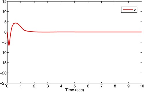
Figure 4. State responses of closed-loop systems (40(40) $\begin{array}{rl}{\dot{x}}_1& =x_2^3+x_1(x_1^{\frac{4}{5}}+x_1^{\frac{4}{3}}),\\ {\dot{x}}_2& =u+x_1(x_1^{\frac{1}{15}}+x_1^{\frac{7}{9}}+x_2^{\frac{1}{4}}+x_2^{\frac{7}{4}}),\\ y& =x_1.\end{array}$(40) )–(42(42) $\begin{array}{rl}\dot{z}& =-u-N\left(\right(z+N{x}_1{)}^3+x_1(x_1^{\frac{4}{5}}+x_2^{\frac{4}{3}})),\\ u& =-(10+2x_1)[\left(\right(z+N{x}_1{)}^3\\ & +(2+x_1)(x_1^{\frac{4}{5}}+x_1^{\frac{4}{3}}){)}^{1/12}\\ & +\left(\right(z+N{x}_1{)}^3+(2+x_1)(x_1^{\frac{4}{5}}+x_1^{\frac{4}{3}}){)}^{7/12}].\end{array}$(42) ) starting from $(1,2,0)$.

For the initial condition $\left[x_1\right(0),x_2(0),z(0\left)\right]=[1,2,0]$, the simulation results are shown in Figures 1–3. The state response $x_1$ with the controller (41(41) $\begin{array}{rl}\dot{z}& =-M(z+M{x}_1+x_1(x_1^{\frac{4}{5}}+x_2^{\frac{4}{3}}\left)\right),\\ u& =-(2+0.5x_1)[(z+M{x}_1+(2+x_1\left)\right(x_1^{\frac{4}{5}}+x_1^{\frac{4}{3}}){)}^{3/4}\\ & +(z+M{x}_1+(2+x_1\left)\right(x_1^{\frac{4}{5}}+x_1^{\frac{4}{3}}){)}^{7/12}],\end{array}$(41) ) is shown in Figure 1. The state response $x_2$ with the controller (41(41) $\begin{array}{rl}\dot{z}& =-M(z+M{x}_1+x_1(x_1^{\frac{4}{5}}+x_2^{\frac{4}{3}}\left)\right),\\ u& =-(2+0.5x_1)[(z+M{x}_1+(2+x_1\left)\right(x_1^{\frac{4}{5}}+x_1^{\frac{4}{3}}){)}^{3/4}\\ & +(z+M{x}_1+(2+x_1\left)\right(x_1^{\frac{4}{5}}+x_1^{\frac{4}{3}}){)}^{7/12}],\end{array}$(41) ) is shown in Figure 2. The state observer z is depicted in Figure 3. It is pointed out that the numerical example can also be designed according to the observer design scheme mentioned in Remark 3.2. The state responses of closed-loop systems (40(40) $\begin{array}{rl}{\dot{x}}_1& =x_2^3+x_1(x_1^{\frac{4}{5}}+x_1^{\frac{4}{3}}),\\ {\dot{x}}_2& =u+x_1(x_1^{\frac{1}{15}}+x_1^{\frac{7}{9}}+x_2^{\frac{1}{4}}+x_2^{\frac{7}{4}}),\\ y& =x_1.\end{array}$(40) )–(42(42) $\begin{array}{rl}\dot{z}& =-u-N\left(\right(z+N{x}_1{)}^3+x_1(x_1^{\frac{4}{5}}+x_2^{\frac{4}{3}})),\\ u& =-(10+2x_1)[\left(\right(z+N{x}_1{)}^3\\ & +(2+x_1)(x_1^{\frac{4}{5}}+x_1^{\frac{4}{3}}){)}^{1/12}\\ & +\left(\right(z+N{x}_1{)}^3+(2+x_1)(x_1^{\frac{4}{5}}+x_1^{\frac{4}{3}}){)}^{7/12}].\end{array}$(42) ) starting from $(1,2,0)$ are shown in Figure 4. (42) $\begin{array}{rl}\dot{z}& =-u-N\left(\right(z+N{x}_1{)}^3+x_1(x_1^{\frac{4}{5}}+x_2^{\frac{4}{3}})),\\ u& =-(10+2x_1)[\left(\right(z+N{x}_1{)}^3\\ & +(2+x_1)(x_1^{\frac{4}{5}}+x_1^{\frac{4}{3}}){)}^{1/12}\\ & +\left(\right(z+N{x}_1{)}^3+(2+x_1)(x_1^{\frac{4}{5}}+x_1^{\frac{4}{3}}){)}^{7/12}].\end{array}$(42)

5. Conclusion

In this article, we have studied global stabilization by output feedback for second-order nonlinear systems with high- and low-order nonlinearities. Nonlinear assumption is more general, so we deal with a larger class of nonlinear system in this article. With the hope of the technique of adding one power integrator, we have exploited a reduced-order design approach for designing a feedback control law, which guarantees the global stability of the corresponding closed-loop system. In addition, our design method in this article is quite different from the homogeneous methods used in most of the existing results. Moreover, an example is given to show the effectiveness of our design scheme. In the future, we will consider output feedback finite-time stabilization of nonlinear systems with polynomial nonlinearities.

Disclosure statement

No potential conflict of interest was reported by the authors.

Additional information

Funding

This work was supported by the National Natural Science Foundation of China (Grant No. 11661065) and the Scientific Research Fund of Jiangxi Provincial Education Department (Grant Nos. GJJ181101 and GJJ171135).

References

- Qian CJ, Lin W. Recursive observer design, homogeneous approximation, and nonsmooth output feedback stabilization of nonlinear systems. IEEE Trans Autom Control. 2006;51:1457–1471. doi: 10.1109/TAC.2006.880955
- Qian CJ, Lin W. Smooth output feedback stabilization of planar systems without controllable/observable linearization. IEEE Trans Autom Control. 2002;47(12):2068–2073. doi: 10.1109/TAC.2002.805690
- Qian CJ, Li J. Global finite-time stabilization by output feedback for planar systems without observable linearization. IEEE Trans Autom Control. 2005;50:885–890. doi: 10.1109/TAC.2005.849253
- Qian CJ, Lin W. Nonsmooth output feedback stabilization of a class of genuinely nonlinear systems in the plane. IEEE Trans Autom Control. 2003;48(10):1824–1829. doi: 10.1109/TAC.2003.817930
- Lei H, Lin W. Robust control of uncertain systems with polynomial nonlinearity by output feedback. Int J Robust Nonlinear Control. 2009;19:692–723. doi: 10.1002/rnc.1349
- Jiang MM, Zhang KM, Xie XJ. Output feedback stabilization of high-order nonlinear time-delay systems with low-order and high-order nonlinearities. IEEE/CAA J Autom Sin. 2018;99:1–16.
- Yang B, Lin W. Robust output feedback stabilization of uncertain nonlinear systems with uncontrollable and unobservable linearization. IEEE Trans Autom Control. 2005;50(5):619–630. doi: 10.1109/TAC.2005.847084
- Li J, Qian CJ. Global finite-time stabilization by dynamic output feedback for a class of continuous nonlinear systems. IEEE Trans Autom Control. 2006;51:879–884. doi: 10.1109/TAC.2006.874991
- Shen YJ, Huang YH, Gu JS. Global finite-time observers for Lipschitz nonlinear systems. IEEE Trans Autom Control. 2011;56:418–424. doi: 10.1109/TAC.2010.2088610
- Li J, Qian CJ, Frye MT. A dual-observer design for global output feedback stabilization of nonlinear systems with low-order and high-order nonlinearities. Int J Robust Nonlinear Control. 2009;19:1697–1720. doi: 10.1002/rnc.1401
- Wang XY, Qian CJ, Li SH. A dual-observer approach for global output feedback stabilization of planar nonlinear systems with output-dependent growth rates. Int J Robust Nonlinear Control. 2015;25:3818–3830. doi: 10.1002/rnc.3292
- Gao FZ, Yuan FS, Wu YQ. Global stabilisation of high-order non-linear systems with time-varying delays. IET Control Theory Appl. 2013;7(13):1737–1744. doi: 10.1049/iet-cta.2013.0435
- Liu L, Xie XJ. Output-feedback stabilization for stochastic high-order nonlinear systems with time-varying delay. Automatica. 2011;47:2772–2779. doi: 10.1016/j.automatica.2011.09.014
- Man YC, Liu YG. Global output-feedback stabilization for a class of uncertain time-varying nonlinear systems. Syst Control Lett. 2016;90:20–30. doi: 10.1016/j.sysconle.2015.09.014
- Jia RT, Qian CJ, Zhai JY. Semi-global stabilisation of uncertain non-linear systems by homogeneous output feedback controllers. IET Control Theory Appl. 2012;6(1):165–172. doi: 10.1049/iet-cta.2010.0503
- Jiang MM, Xie XJ, Zhang KM. Finite-time output feedback stabilisation of high-order uncertain nonlinear systems. Int J Control. 2018;91:1338–1349. doi: 10.1080/00207179.2017.1314021
- Li J, Qian CJ, Ding SH. Global finite-time stabilisation by output feedback for a class of uncertain nonlinear systems. Int J Control. 2010;83:2241–2252. doi: 10.1080/00207179.2010.511658
- Su YX, Zheng CH. Robust finite-time output feedback control of perturbed double integrator. Automatica. 2015;60:86–91. doi: 10.1016/j.automatica.2015.07.008
- Zhai JY. Global finite-time output feedback stabilisation for a class of uncertain nontriangular nonlinear system. Int J Syst Sci. 2014;45(3):637–646. doi: 10.1080/00207721.2012.724113
- Zhai JY, Song ZB. Global finite-time stabilization for a class of switched nonlinear systems via output feedback. Int J Control Autom Syst. 2017;15(5):1975–1982. doi: 10.1007/s12555-016-0490-z
- Wang XH. Global finite-time stabilization of a class of nonlinear system based on a dynamic gain approach. Math Methods Appl Sci. 2020;43(1):269–280. doi: 10.1002/mma.5874
- Gao FZ, Wu YQ. Finite-time output feedback stabilisation of chained-form systems with inputs saturation. Int J Control. 2017;90(7):1466–1477. doi: 10.1080/00207179.2016.1209564
- Zhai JY, Song ZB, Fei SM, et al. Global finite-time output feedback stabilisation for a class of switched high-order nonlinear systems. Int J Control. 2018;91:170–180. doi: 10.1080/00207179.2016.1274429
- Tunç O, Tunç C. On the asymptotic stability of solutions of stochastic differential delay equations of second order. J Taibah Univ Sci. 2019;13(1):875–882. doi: 10.1080/16583655.2019.1652453
- Tunç O, Tunç C. Qualitative analysis for a variable delay system of differential equations of second order. J Taibah Univ Sci. 2019;13(1):468–477. doi: 10.1080/16583655.2019.1595359
- Bahaa GM, Hamiaz A. Optimal control problem for coupled time-fractional diffusion systems with final observations. J Taibah Univ Sci. 2019;13(1):124–135. doi: 10.1080/16583655.2018.1545560
- Li GQ, Lin Y. Robust output feedback stabilization of nonlinear systems with low-order and high-order nonlinearities. Int J Robust Nonlinear Control. 2016;26:1919–1943. doi: 10.1002/rnc.3389
- Zhang XH, Xie XJ. Global state feedback stabilisation of nonlinear systems with high-order and low-order nonlinearities. Int J Control. 2014;87(3):642–652. doi: 10.1080/00207179.2013.852252
- Sun ZY, Liu ZG, Zhang XH. New results on global stabilization for time-delay nonlinear systems with low-order and high-order growth conditions. Int J Robust Nonlinear Control. 2015;25:878–899. doi: 10.1002/rnc.3115
- Zhang KM, Zhang XH. Finite-time stabilisation for high-order nonlinear systems with low-order and high-order nonlinearities. Int J Control. 2015;88(8):1576–1585. doi: 10.1080/00207179.2015.1011697
- Gao FZ, Wu YQ. Global state feedback stabilisation for a class of more general high-order non-linear systems. IET Control Theory Appl. 2017;8(16):1648–1655. doi: 10.1049/iet-cta.2014.0175
- Gao FZ, Wu YQ, Yu X. Global state feedback stabilisation of stochastic high-order nonlinear systems with high-order and low-order nonlinearities. Int J Syst Sci. 2016;7(16):3846–3856. doi: 10.1080/00207721.2015.1129678
- Qian CJ, Lin W. Non-Lipschitz continuous stabilizers for nonlinear systems with uncontrollable unstable linearization. Syst Control Lett. 2001;42:185–200. doi: 10.1016/S0167-6911(00)00089-X