A semi-analytical method to solve family of Kuramoto–Sivashinsky equations

Abstract

In this article, a semi-analytical technique is implemented to solve Kuramoto–Sivashinsky equations. The present method is the combination of two well-known methods namely Laplace transform method and variational iteration method. This hybrid property of the proposed method reduces the numbers of calculations and materials. The accuracy and applicability of the suggested method is confirmed through illustration examples. The accuracy of the proposed method is described in terms of absolute error. It is investigated through graphs and tables that the Laplace transformation and variational iteration method (LVIM) solutions are in good agreement with the exact solution of the problems. The LVIM solutions are also obtained at different fractional-order of the derivative. It is observed through graphs and tables that the fractional-order solutions are convergent to an integer solution as fractional-orders approaches to an integer-order of the problems. In conclusion, the overall implementation of the present method support the validity of the suggested method. Due to simple, straightforward and accurate implementation, the present method can be extended to other non-linear fractional partial differential equations.

Keywords:

• Variational iteration method
• Laplace transform
• Lagrange multiplier
• Kuramoto–Sivashinsky equations

1. Introduction

Over recent years, the theory of fractional calculus (FC) has drawn global attention to its implementations over complex systems. According to the fractional derivative principles, the simulation of significant-world problems containing fractional-order derivatives provides better predictability compared to modelling involving integer-order derivatives. FC defines the background and non-local dispersed effects of any physical system, in specific phenomenon related to the analysis of chaos in wave motion, solitary waves, phase turbulence in reaction–diffusion schemes [1–4], wrinkled flame front propagation [5], chaotic drifting waves induced by photon collision [6], time fractional-coupled mKdV equation [7–9], fractional-order wave equations [10] and fractional space–time diffusion equation [11–13].

In 1977, Gregory I. Sivashinsky measured a scenario for such a laminar flaming front. An other researcher, Yoshiki Kuramoto, created a certain problem when simultaneously designing diffusion-induced chaotic in a three-dimensional experiment of the Belousov–Zabotinskii transformation [4,14–16]. Their combined result is named the Kuramoto–Sivashinsky (KS) model. This system defines the changes in that burning front orientation, the motion of the liquid down a circular surface and a dynamically particular oscillating chemical compound in a homogeneous fluid [17–19]. It introduces chaotic behaviour, requiring a result such as moving waves travelling to a finite space domain without altering size. That has a variety of implementations in a range of conceptual ideas, along with response diffusion systems [20], thin film hydrodynamics [21] and front burn instability [22], long waves on functionality among a couple vicious fluids [23].

As stated in [24], the generalized KS equation is a form of non-linear partial differential equations (PDEs) naturally found in the research of fluid materials that displays a chaotic type of conduct. (1) $\frac{{\mathrm{\partial }}^{\kappa }\mu }{\mathrm{\partial }{t}^{\kappa }}+\mu \frac{\mathrm{\partial }\mu }{\mathrm{\partial }x}+\eta \frac{{\mathrm{\partial }}^2\mu }{\mathrm{\partial }{x}^2}+\theta \frac{{\mathrm{\partial }}^3\mu }{\mathrm{\partial }{x}^3}+\omega \frac{{\mathrm{\partial }}^4\mu }{\mathrm{\partial }{x}^4}=0,$(1) where η, θ and ω are non-zero constants.

For $\theta =0$, Equation (1(1) $\frac{{\mathrm{\partial }}^{\kappa }\mu }{\mathrm{\partial }{t}^{\kappa }}+\mu \frac{\mathrm{\partial }\mu }{\mathrm{\partial }x}+\eta \frac{{\mathrm{\partial }}^2\mu }{\mathrm{\partial }{x}^2}+\theta \frac{{\mathrm{\partial }}^3\mu }{\mathrm{\partial }{x}^3}+\omega \frac{{\mathrm{\partial }}^4\mu }{\mathrm{\partial }{x}^4}=0,$(1) ) is named the KS model, a canon non-linear reproduction equation that arises in a multitude of physical situations. For $\eta =\omega =1$ and $\theta =0$, it denotes pattern structure designs on unbalanced flame fronts and thin hydrodynamic movies, Equation (1(1) $\frac{{\mathrm{\partial }}^{\kappa }\mu }{\mathrm{\partial }{t}^{\kappa }}+\mu \frac{\mathrm{\partial }\mu }{\mathrm{\partial }x}+\eta \frac{{\mathrm{\partial }}^2\mu }{\mathrm{\partial }{x}^2}+\theta \frac{{\mathrm{\partial }}^3\mu }{\mathrm{\partial }{x}^3}+\omega \frac{{\mathrm{\partial }}^4\mu }{\mathrm{\partial }{x}^4}=0,$(1) ) has been researched extensively [25,26].

In past decade, multiple types of mathematical systems have been produced for the numerical methods of time dependent PDEs [27]. The KSE has been studied by different methods, such as, homotopy analysis method [28], Runge-Kutta method [29], finite difference scheme [30], B-spline functions [31], mesh-free numerical method [32], Reduced differential transform method [33], Lattice Boltzmann method [34], Quasi-exact KS equation solutions [35], Sub-equation Method [36] and modified tanh–coth method [37].

A Lagrange multiplier method has been commonly used to solve a variety of non-linear equations [38]. This occurs in physics and mathematics or other related areas but has been developed as a basic analytical technique, i.e. a variational iteration method (VIM) for modelling differential equations [39]. The VIM was first suggested by He [40] and was effectively implemented in dealing with heat transform problems [40–42]. The fractional variational iteration technique (FVIM) was developed via modified Riemann–Liouville derivative in 2010 [43]. Recently, a procedure combined in this sense VIM and Laplace transform technique was proposed [44,45] and Wu developed a modification via FC and Laplace transformation [46]. Laplace transformation and variational iteration method (LVIM) for solving non-linear PDEs [47] and system of fractional PDEs [48,49].

In the present research work, we implemented a hybrid technique for the solution of family of fractional-order Kuramoto–Sivashinsky equations. The present technique is the combination of two well-known methods namely LVIM is discussed in Section 3 of the paper. The convergence analysis of the suggested method is discussed in Theorem 5.1 of the manuscript. For the purpose of the validity of the current method, some illustrative examples are presented. The graphical representations of Examples 6.1, 6.2 and 6.3 in the paper have shown close contact of LVIM solutions with the exact solutions of the problems. Moreover, the LVIM solutions are calculated at different fractional-order of the targeted problems. It is investigated that the fractional-order solutions are converged to an integer-order solution for the problem as fractional-orders approaches to an integer-order. The accuracy of the proposed methods analysed with the help of Tables 1–3 in term absolute error (AE). From the table, it is clear that LVIM has the desired degree of accuracy. The overall, discussion and numerical implementation of the current method have suggested extending that it can be extended easily to solve other fractional-order differential equations.

Table 1. The LVIM and reproducing Kernel Hilbert space method (RKHSM) their corresponding absolute errors (AE) at different fractional-order κ of Example 6.1.

t	x	$\kappa =0.75$	$\kappa =1$	Exact	$AE\left(RKHSM\right)$ [50]	$AE\left(LVIM\right)$
0.1	1	2.8742118170	2.4972002150	2.497723372	5.55E−04	5.55E−04
	2	−2.323008368	−2.4484441260	−2.448081016	3.66E−04	3.66E−04
	3	−3.708744132	−3.7332570560	−3.733169900	1.48E−04	1.48E−04
	4	−3.956558383	−3.9603797970	−3.960365210	1.51E−04	1.51E−04
	5	−3.993901852	−3.9944471490	−3.994445020	2.69E−05	2.68E−05
0.5	1	4.1763182870	3.11557827900	3.127995924	2.03E−02	2.03E−02
	2	−1.870376356	−2.2425245620	−2.232914697	2.56E−03	2.56E−03
	3	−3.618654104	−3.6930007580	−3.690623590	6.48E−03	2.48E−03
	4	−3.942412918	−3.9541031590	−3.953700660	1.10E−04	1.10E−04
	5	−3.991877906	−3.9935514540	−3.993492270	1.63E−05	1.61E−05

Table 2. LVIM and AE at distinct fractional-order κ of Example 6.2.

t	x	$\kappa =0.75$	$\kappa =1$	Exact	$AE(\kappa =1)$
0.1	1	−6.846609544	−7.072056697	−7.166875017	9.48E−02
	2	−4.427777312	−4.613806338	−4.615821774	2.01E−03
	3	−1.148219426	−1.222770396	−1.204329860	1.84E−02
	4	0.525722483	0.501353776	0.511441910	1.00E−02
	5	1.181394942	1.173387101	1.177359330	3.97E−03
0.5	1	−5.539425367	−6.701156428	−7.181246074	4.80E−01
	2	−3.880210462	−4.308828578	−4.319499133	1.06E−02
	3	−0.861200835	−1.100276823	−1.021195210	7.90E−02
	4	0.613459178	0.541362538	0.586878520	4.55E−02
	5	1.209030933	1.186524333	1.204762410	1.82E−02

Table 3. LVIM and AE at distinct fractional-order κ of Example 6.3.

t	x	$\kappa =0.75$	$\kappa =1$	Exact	$AE(\kappa =1)$
0.1	1	−0.52531204	−0.535712512	−0.537461933	1.74E−03
	2	2.048065728	2.089519721	2.098276512	8.75E−03
	3	4.394074956	4.427256229	4.434021119	6.76E−03
	4	5.519284464	5.534215367	5.537207116	2.99E−03
	5	5.951376432	5.956968910	5.958082037	1.11E−03
0.5	1	−0.49268345	−0.527604267	−0.536307927	8.70E−03
	2	1.936408163	2.056955205	2.100455409	4.35E−02
	3	4.300387227	4.401361744	4.435249580	3.38E−02
	4	5.475218700	5.522623576	5.537703222	1.50E−02
	5	5.934596588	5.952636153	5.958261217	5.62E−03

2. Preliminaries and definitions

2.1. Definition

Laplace transformation of $\tilde{\rho }\left(t\right)$, $t>0$ represented as [51,52] (2) $Q\left(s\right)=\mathcal{L}\left[\tilde{\rho }\left(t\right)\right]={\int }_0^{\mathrm{\infty }}{\mathrm{e}}^{-st}\tilde{\rho }\left(t\right)\mathrm{d}t.$(2)

2.2. Definition

The Laplace transforms in forms of convolution (3) $\mathcal{L}[{\tilde{\rho }}_1\ast {\tilde{\rho }}_2]=\mathcal{L}\left[{\tilde{\rho }}_1\right(t\left)\right]\ast \mathcal{L}\left[{\tilde{\rho }}_2\right(t\left)\right],$(3) here ${\tilde{\rho }}_1\ast {\tilde{\rho }}_2$, define the convolution between ${\tilde{\rho }}_1$ and ${\tilde{\rho }}_2$, (4) $({\tilde{\rho }}_1\ast {\tilde{\rho }}_2)t={\int }_0^{\tau }{\tilde{\rho }}_1\left(\tau \right){\tilde{\rho }}_2(t-\tau )\mathrm{d}t.$(4) Laplace transform is a fractional derivative (5) $\begin{array}{rl}\mathcal{L}\left(D_t^{\kappa }\tilde{\rho }\left(t\right)\right)& =s^{\kappa }Q\left(s\right)-\sum _{k=0}^{n-1}{s}^{\kappa -1-k}{\tilde{\rho }}^{\left(k\right)}\left(0\right),\\ & \times n-1<\kappa <n,\end{array}$(5) where $Q\left(s\right)$ is the Laplace transformation of $\tilde{\rho }\left(t\right)$.

2.3. Definition

Riemann–Liouville fractional integral [53,54] (6) $I_x^{\kappa }g\left(x\right)=\left\{\begin{array}{ll}g\left(x\right)& \mathrm{i}\mathrm{f}\kappa =0\\ \frac{1}{\mathrm{\Gamma }\left(\kappa \right)}{\int }_0^x(x-\kappa {)}^{\kappa -1}g(\kappa .)\mathrm{d}\kappa & \mathrm{i}\mathrm{f}\kappa >0,\end{array}\right.$(6) where Γ represent the gamma function as, (7) $\mathrm{\Gamma }\left(\kappa \right)={\int }_0^{\mathrm{\infty }}{\mathrm{e}}^{-x}{x}^{\kappa -1}\mathrm{d}x,\kappa \in \mathbb{C},$(7)

2.4. Definition

The following mathematical expression is given to the Caputo of fractional derivative of order κ for $\overline{m}\in \mathbb{N}$, x>0, $g\in {\mathbb{C}}_t$,  $t\ge -1$. (8) $D^{\kappa }g\left(x\right)=\frac{{\mathrm{\partial }}^{\kappa }g\left(x\right)}{\mathrm{\partial }{t}^{\gamma }}=\left\{\begin{array}{l}{I}^{\tilde{m}-\kappa }\left[\frac{{\mathrm{\partial }}^{\kappa }g\left(x\right)}{\mathrm{\partial }{t}^{\kappa }}\right],\\ \mathrm{i}\mathrm{f}\tilde{m}-1<\kappa \le \tilde{m},\tilde{m}\in \mathbb{N}& \\ \frac{{\mathrm{\partial }}^{\kappa }g\left(x\right)}{\mathrm{\partial }{t}^{\kappa }},& \end{array}\right.$(8)

2.5. Lemma

If $\tilde{m}-1<\kappa \le \tilde{m}$ with $\tilde{m}\in \mathbb{N}$ and $g\in {\mathbb{C}}_t$ with $t\ge -1$, then [55] (9) $\begin{array}{rl}{I}^{\kappa }{I}^{a}g\left(x\right)& =I^{\kappa +a}g\left(x\right),a,\kappa \ge 0.\\ I^{\kappa }{x}^{\lambda }& =\frac{\mathrm{\Gamma }(\lambda +1)}{\mathrm{\Gamma }(\gamma +\lambda +1)}{x}^{\kappa +\lambda },\\ & \times \kappa >0,\lambda >-1,x>0.\\ I^{\kappa }{D}^{\kappa }g\left(x\right)& =g\left(x\right)-\sum _{k=0}^{\tilde{m}-1}{g}^{\left(k\right)}\left(0^{+}\right)\frac{x^k}{k!},\\ & \times \mathrm{f}\mathrm{o}\mathrm{r}x>0,\tilde{m}-1<\kappa \le \tilde{m}.\end{array}$(9)

2.6. Definition

Function of Mittag-Leffler, $E_{\kappa }\left(b\right)$ for $\kappa >0$ is defined as (10) $E_{\kappa }\left(b\right)=\sum _{\tilde{m}=0}^{\mathrm{\infty }}\frac{b^{\tilde{m}}}{\mathrm{\Gamma }\left(\kappa \tilde{m}+1\right)},\kappa >0b\in \mathbb{C},$(10)

3. Basics of the VIM

In order to explain the basic knowledge of the method, consider the following common non-linear scheme: (11) $\frac{{\mathrm{\partial }}^{\kappa }\mu }{\mathrm{\partial }{t}^{\kappa }}+\mathcal{R}\left(\mu \right)+\mathcal{N}\left(\mu \right)=\mathcal{P}\left(t\right),$(11) where $\mu =\mu \left(t\right)$, $\mathcal{R}$ is a linear operator, $\mathcal{N}$ is a non-linear operator and $\mathcal{P}$ is a given continuous function.

The basic character of the technique is to construct the following correction well-designed for Equation(11(11) $\frac{{\mathrm{\partial }}^{\kappa }\mu }{\mathrm{\partial }{t}^{\kappa }}+\mathcal{R}\left(\mu \right)+\mathcal{N}\left(\mu \right)=\mathcal{P}\left(t\right),$(11) ): (12) $\begin{array}{rl}{\mu }_{m+1}& ={\mu }_m+{\int }_0^t\lambda (t,\tau )\left(\frac{{\mathrm{\partial }}^{\kappa }\mu }{\mathrm{\partial }{\tau }^{\kappa }}+\mathcal{R}\left({\mu }_m\right)\right.\\ & \left.\phantom{\frac{{\mathrm{\partial }}^{\kappa }\mu }{\mathrm{\partial }{\tau }^{\kappa }}}+\mathcal{N}\left({\mu }_m\right)-\mathcal{P}\left(\tau \right)\right)\mathrm{d}\tau ,\end{array}$(12) where $\lambda (t,\tau )$ is called the general Lagrange multiplier and ${\mu }_m$ is the nth-order estimated solution.

4. The procedure of LVIM

In the case of an algebraic equation, let us revisit the original idea of the Lagrange multipliers. In the first place, an iteration formula for the solution of algebraic equation $g\left(x\right)=0$ can be constructed as (13) ${\chi }_{m+1}={\chi }_m+\lambda g\left({\chi }_m\right).$(13) The optimal situation for the maximum $\kappa {\chi }_{m+1}/\kappa {\chi }_m=0$ leads to (14) $\lambda =-\frac{1}{g^{\mathrm{\prime }}\left({\chi }_m\right)},$(14) In which κ is a classic variational operator. From (13(13) ${\chi }_{m+1}={\chi }_m+\lambda g\left({\chi }_m\right).$(13) ) and (14(14) $\lambda =-\frac{1}{g^{\mathrm{\prime }}\left({\chi }_m\right)},$(14) ), we can discover the estimated method ${\chi }_{m+1}$ by the iterative system for (14(14) $\lambda =-\frac{1}{g^{\mathrm{\prime }}\left({\chi }_m\right)},$(14) ) for a specified original value ${\chi }_m$. (15) ${\chi }_{m+1}={\chi }_m-\frac{g\left({\chi }_m\right)}{g^{\mathrm{\prime }}\left({\chi }_m\right)},g^{\mathrm{\prime }}\left({\chi }_0\right)\ne 0,m=0,1,2,\dots$(15) Now they expand its concept to find the unidentified Lagrange multiplier. The primary stage is to bring the Laplace transformation to Equation (13(13) ${\chi }_{m+1}={\chi }_m+\lambda g\left({\chi }_m\right).$(13) ) first. Therefore, the linear portion is converted in to an algebraic statement as given: (16) $\begin{array}{rl}& s^{\kappa }\mu \left(s\right)-{\mu }^{\kappa -1}\left(0\right)-s^{\kappa -1}\mu \left(0\right)\\ & \times +\text{£}\left[\mathcal{R}\left(\mu \right)+\mathcal{N}\left(\mu \right)-\mathcal{P}\left(\mu \right)\right]=0,\end{array}$(16) where $\mu \left(s\right)=\text{£}\left(\mu \right(t\left)\right)={\int }_0^{\mathrm{\infty }}{\mathrm{e}}^{-st}\mu \left(t\right)\mathrm{d}t$.

The iteration algorithm (16(16) $\begin{array}{rl}& s^{\kappa }\mu \left(s\right)-{\mu }^{\kappa -1}\left(0\right)-s^{\kappa -1}\mu \left(0\right)\\ & \times +\text{£}\left[\mathcal{R}\left(\mu \right)+\mathcal{N}\left(\mu \right)-\mathcal{P}\left(\mu \right)\right]=0,\end{array}$(16) ) are used to recommend the key iterative system that included a Lagrange multiplier as (17) $\begin{array}{rl}{\mu }_{m+1}\left(s\right)& ={\mu }_m\left(s\right)+\lambda \left(s\right)\left[s^{\kappa }\mu \right(s)-{\mu }^{\kappa -1}(0)-s^{\kappa -1}\mu (0)\\ & +\text{£}\left[\mathcal{R}\left(\mu \right)+\mathcal{N}\left(\mu \right)-\mathcal{P}\left(\mu \right)\right].\end{array}$(17) Considered $\text{£}\left[\mathcal{R}\right(\mu )+\mathcal{N}(\mu \left)\right]$ as limited conditions, a Lagrange calculation can be derived as (18) $\lambda \left(s\right)=-\frac{1}{s^{\kappa }}.$(18) Because of Equation (18(18) $\lambda \left(s\right)=-\frac{1}{s^{\kappa }}.$(18) ) and the inverse Laplace transformation ${\text{£}}^{-1}$, iteration method (5(5) $\begin{array}{rl}\mathcal{L}\left(D_t^{\kappa }\tilde{\rho }\left(t\right)\right)& =s^{\kappa }Q\left(s\right)-\sum _{k=0}^{n-1}{s}^{\kappa -1-k}{\tilde{\rho }}^{\left(k\right)}\left(0\right),\\ & \times n-1<\kappa <n,\end{array}$(5) ) can also be expressly stated as (19) $\begin{array}{rl}{\mu }_{m+1}\left(t\right)& ={\mu }_m\left(t\right)-{\text{£}}^{-1}\left[\frac{1}{s^{\kappa }}\left\{s^{\kappa }\mu \left(s\right)-{\mu }^{\kappa -1}\left(0\right)\right.\right.\\ & \left.\left.-s^{\kappa -1}\mu \left(0\right)+\text{£}\left(\mathcal{R}\left(\mu \right)+\mathcal{N}\left(\mu \right)-\mathcal{P}\left(\mu \right)\right)\right\}\right].\end{array}$(19) The Laplace solution for equation (19(19) $\begin{array}{rl}{\mu }_{m+1}\left(t\right)& ={\mu }_m\left(t\right)-{\text{£}}^{-1}\left[\frac{1}{s^{\kappa }}\left\{s^{\kappa }\mu \left(s\right)-{\mu }^{\kappa -1}\left(0\right)\right.\right.\\ & \left.\left.-s^{\kappa -1}\mu \left(0\right)+\text{£}\left(\mathcal{R}\left(\mu \right)+\mathcal{N}\left(\mu \right)-\mathcal{P}\left(\mu \right)\right)\right\}\right].\end{array}$(19) ) represent the general iterative formula for the targeted problem.

5. Convergence analysis

Theorem 5.1

Let χ and $\mathcal{Y}$ be two Banach spaces and $T:\chi \to \mathcal{Y}$ be a contractive non-linear operator, such that for all $u;u^{\ast }\in ;\chi ,||T\left(u\right)-T\left(u^{\ast }\right)||\le K||u-u^{\ast }||,$ 0<K<1 [56].

Then, in view of Banach contraction theorem, T has a unique fixed point u, such that $Tu=u:$ Let us write the generated series (19(19) $\begin{array}{rl}{\mu }_{m+1}\left(t\right)& ={\mu }_m\left(t\right)-{\text{£}}^{-1}\left[\frac{1}{s^{\kappa }}\left\{s^{\kappa }\mu \left(s\right)-{\mu }^{\kappa -1}\left(0\right)\right.\right.\\ & \left.\left.-s^{\kappa -1}\mu \left(0\right)+\text{£}\left(\mathcal{R}\left(\mu \right)+\mathcal{N}\left(\mu \right)-\mathcal{P}\left(\mu \right)\right)\right\}\right].\end{array}$(19) ), by the Laplace variational iteration method as ${\chi }_m=T\left({\chi }_{m-1}\right),{\chi }_{m-1}=\sum _{j=1}^{m-1}{u}_j,j=0,1,2,\dots$ and supposed that ${\chi }_0=u_0\in {\mathcal{S}}_p\left(u\right),$ where ${\mathcal{S}}_p\left(u\right)=\{u^{\ast }\in \chi :||u-u^{\ast }||<p\}$ then, we have $\begin{array}{rl}& \left(B_1\right){\chi }_m\in {\mathcal{S}}_p\left(u\right)\\ & \left(B_2\right)\underset{m\to \mathrm{\infty }}{lim}{\chi }_n=u.\end{array}$

Proof.

$\left(B_1\right)$ In view of mathematical induction for m = 1, we have $||{\chi }_1-u_1||=||T({\chi }_0-T(u\left)\right)||\le K||u_0-u||.$ Let the result is true for m−1, then $||{\chi }_{m-1}-u||\le K^{m-1}||u_0-u||.$ We have $\begin{array}{rl}||{\chi }_m-u||& =||T({\chi }_{m-1}-T(u\left)\right)||\le K||{\chi }_{m-1}-u||\\ & \le K^m||u_0-u||.\end{array}$ Hence, using $\left(B_1\right)$, we have $||{\chi }_m-u||\le K^m||u_0-u||\le K^{m}p<p,$ which implies that ${\chi }_m\in {\mathcal{S}}_p\left(u\right)$. $\left(B_2\right)$: Since $||{\chi }_m-u||\le K^m||u_0-u||$ and as a $\underset{m\to \mathrm{\infty }}{lim}{K}^m=0$.

Therefore, we have $\underset{m\to \mathrm{\infty }}{lim}||u_n-u||=0\Rightarrow \underset{m\to \mathrm{\infty }}{lim}{u}_n=u$.

6. Numerical examples

Example 6.1

In this instance, we discover the equation KS as described by $\eta =\theta =1$ and $\omega =4$ [31,32,50]. (20) $\frac{{\mathrm{\partial }}^{\kappa }\mu }{\mathrm{\partial }{t}^{\kappa }}+\mu \frac{\mathrm{\partial }\mu }{\mathrm{\partial }x}+\eta \frac{{\mathrm{\partial }}^2\mu }{\mathrm{\partial }{x}^2}+\theta \frac{{\mathrm{\partial }}^3\mu }{\mathrm{\partial }{x}^3}+\omega \frac{{\mathrm{\partial }}^4\mu }{\mathrm{\partial }{x}^4}=0,$(20) with initial condition $\begin{array}{rl}{\mu }_0(x,0)& =11+15\tanh \left(\frac{-1}{2}x\right)-15{\tanh }^2\left(\frac{-1}{2}x\right)\\ & -15{\tanh }^3\left(\frac{-1}{2}x\right).\end{array}$ Using LVIM on both sides equation (20(20) $\frac{{\mathrm{\partial }}^{\kappa }\mu }{\mathrm{\partial }{t}^{\kappa }}+\mu \frac{\mathrm{\partial }\mu }{\mathrm{\partial }x}+\eta \frac{{\mathrm{\partial }}^2\mu }{\mathrm{\partial }{x}^2}+\theta \frac{{\mathrm{\partial }}^3\mu }{\mathrm{\partial }{x}^3}+\omega \frac{{\mathrm{\partial }}^4\mu }{\mathrm{\partial }{x}^4}=0,$(20) ), we get (21) $\begin{array}{rl}{\mu }_{m+1}(x,t)& ={\text{£}}^{-1}\left[\frac{u_m(x,t)}{s}\right]\\ & +{\text{£}}^{-1}\left[\lambda \left(s\right)\left\{s^{\kappa }\frac{\mathrm{\partial }{\mu }_m}{\mathrm{\partial }s}+{\mu }_m\frac{\mathrm{\partial }{\mu }_m}{\mathrm{\partial }x}\right.\right.\\ & +\left.\left.\eta \frac{{\mathrm{\partial }}^2{\mu }_m}{\mathrm{\partial }{x}^2}+\theta \frac{{\mathrm{\partial }}^3{\mu }_m}{\mathrm{\partial }{x}^3}+\omega \frac{{\mathrm{\partial }}^4{\mu }_m}{\mathrm{\partial }{x}^4}\right\}\right],\end{array}$(21) where $\lambda \left(s\right)$ is the Lagrange multiplier (22) $\begin{array}{rl}\lambda \left(s\right)& =\frac{-1}{s^{\kappa }},\\ {\mu }_{m+1}(x,t)& =u_m(x,t)-{\text{£}}^{-1}\left[\frac{1}{s^{\kappa }}\left\{s^{\kappa }\frac{\mathrm{\partial }{\mu }_m}{\mathrm{\partial }s}+{\mu }_m\frac{\mathrm{\partial }{\mu }_m}{\mathrm{\partial }x}\right.\right.\\ & +\left.\left.\eta \frac{{\mathrm{\partial }}^2{\mu }_m}{\mathrm{\partial }{x}^2}+\theta \frac{{\mathrm{\partial }}^3{\mu }_m}{\mathrm{\partial }{x}^3}+\omega \frac{{\mathrm{\partial }}^4{\mu }_m}{\mathrm{\partial }{x}^4}\right\}\right].\end{array}$(22) Now take, $\begin{array}{rl}{\mu }_0(x,t)& =11+15\tanh \left(\frac{-1}{2}x\right)-15{\tanh }^2\left(\frac{-1}{2}x\right)\\ & -15{\tanh }^3\left(\frac{-1}{2}x\right),\end{array}$ consequently, we get, $\begin{array}{rl}{\mu }_1(x,t)& =u_0(x,t)-{\text{£}}^{-1}\left[\frac{1}{s^{\kappa }}\left\{s^{\kappa }\frac{\mathrm{\partial }{\mu }_0}{\mathrm{\partial }s}+{\mu }_0\frac{\mathrm{\partial }{\mu }_0}{\mathrm{\partial }x}\right.\right.\\ & +\left.\left.\eta \frac{{\mathrm{\partial }}^2{\mu }_0}{\mathrm{\partial }{x}^2}+\theta \frac{{\mathrm{\partial }}^3{\mu }_0}{\mathrm{\partial }{x}^3}+\omega \frac{{\mathrm{\partial }}^4{\mu }_0}{\mathrm{\partial }{x}^4}\right\}\right],\\ {\mu }_1(x,t)& =11+15\tanh \left(\frac{-1}{2}x\right)-15{\tanh }^2\left(\frac{-1}{2}x\right)\\ & -15{\tanh }^3\left(\frac{-1}{2}x\right)\\ & -\frac{60\left(-2+\cosh \left(x\right)-\sinh \left(x\right)\right)}{{\cosh }^2\left(x\right)+2\cosh \left(x\right)+1}\frac{t^{\kappa }}{\mathrm{\Gamma }(\kappa +1)},\\ {\mu }_2(x,t)& =u_1(x,t)-{\text{£}}^{-1}\left[\frac{1}{s^{\kappa }}\left\{s^{\kappa }\frac{\mathrm{\partial }{\mu }_1}{\mathrm{\partial }s}+{\mu }_1\frac{\mathrm{\partial }{\mu }_1}{\mathrm{\partial }x}\right.\right.\\ & +\left.\left.\eta \frac{{\mathrm{\partial }}^2{\mu }_1}{\mathrm{\partial }{x}^2}+\theta \frac{{\mathrm{\partial }}^3{\mu }_1}{\mathrm{\partial }{x}^3}+\omega \frac{{\mathrm{\partial }}^4{\mu }_1}{\mathrm{\partial }{x}^4}\right\}\right],\\ {\mu }_2(x,t)& =11+15\tanh \left(\frac{-1}{2}x\right)-15{\tanh }^2\left(\frac{-1}{2}x\right)\\ & -15{\tanh }^3\left(\frac{-1}{2}x\right)\\ & -\frac{60(-2+\cosh (x)-\sinh (x\left)\right)}{{\cosh }^2\left(x\right)+2\cosh \left(x\right)+1}\frac{t^{\kappa }}{\mathrm{\Gamma }(\kappa +1)}\\ & +\frac{\begin{array}{c}60({\cosh }^2(x)-\cosh (x)-\sinh (x)\\ \cosh \left(x\right)-2+5\sinh \left(x\right))\end{array}}{{\cosh }^3\left(x\right)+3{\cosh }^2\left(x\right)+3\cosh \left(x\right)+1}\\ & \times \frac{t^{2\kappa }}{\mathrm{\Gamma }(2\kappa +1)},\end{array}$ and $\begin{array}{rl}{\mu }_3(x,t)& =u_2(x,t)-{\text{£}}^{-1}\left[\frac{1}{s^{\kappa }}\left\{s^{\kappa }\frac{\mathrm{\partial }{\mu }_2}{\mathrm{\partial }s}+{\mu }_2\frac{\mathrm{\partial }{\mu }_2}{\mathrm{\partial }x}\right.\right.\\ & +\left.\left.\eta \frac{{\mathrm{\partial }}^2{\mu }_2}{\mathrm{\partial }{x}^2}+\theta \frac{{\mathrm{\partial }}^3{\mu }_1}{\mathrm{\partial }{x}^3}+\omega \frac{{\mathrm{\partial }}^4{\mu }_2}{\mathrm{\partial }{x}^4}\right\}\right],\\ {\mu }_3(x,t)& =11+15\tanh \left(\frac{-1}{2}x\right)-15{\tanh }^2\left(\frac{-1}{2}x\right)\\ & -15{\tanh }^3\left(\frac{-1}{2}x\right)\\ & -\frac{60(-2+\cosh (x)-\sinh (x\left)\right)}{{\cosh }^2\left(x\right)+2\cosh \left(x\right)+1}\frac{t^{\kappa }}{\mathrm{\Gamma }(\kappa +1)}\\ & \times \frac{\begin{array}{c}60({\cosh }^2(x)-\cosh (x)-\sinh (x)\\ \cosh \left(x\right)-2+5\sinh \left(x\right))\end{array}}{{\cosh }^3\left(x\right)+3{\cosh }^2\left(x\right)+3\cosh \left(x\right)+1}\\ & \times \frac{t^{2\kappa }}{\mathrm{\Gamma }(2\kappa +1)}\\ & \times \frac{\begin{array}{c}{\cosh }^2\left(x\right)-13\cosh \left(x\right)-\sinh \left(x\right)\cosh \left(x\right)\\ +16+5\sinh \left(x\right)\end{array}}{{\cosh }^3\left(x\right)+3{\cosh }^2\left(x\right)+3\cosh \left(x\right)+1}\\ & \times \frac{t^{3\kappa }}{\mathrm{\Gamma }(3\kappa +1)},\\ & ⋮\end{array}$ For $m=3,4,5\dots$ $\begin{array}{rl}{\mu }_{m+1}(x,t)& =u_m(x,t)-{\text{£}}^{-1}\left[\frac{1}{s^{\kappa }}\left\{s^{\kappa }\frac{\mathrm{\partial }{\mu }_m}{\mathrm{\partial }s}+{\mu }_m\frac{\mathrm{\partial }{\mu }_m}{\mathrm{\partial }x}\right.\right.\\ & +\left.\left.\eta \frac{{\mathrm{\partial }}^2{\mu }_m}{\mathrm{\partial }{x}^2}+\theta \frac{{\mathrm{\partial }}^3{\mu }_m}{\mathrm{\partial }{x}^3}+\omega \frac{{\mathrm{\partial }}^4{\mu }_m}{\mathrm{\partial }{x}^4}\right\}\right].\end{array}$ The exact result is (23) $\mu (x,t)=11+15\tanh \mathrm{\Phi }-15{\tanh }^2\mathrm{\Phi }-15{\tanh }^3\mathrm{\Phi },$(23) then $\mathrm{\Phi }=-\frac{1}{2}x+t$, on the interval $[-1,1]$.

Example 6.2

The KS equation as defined by $\eta =2$ $\theta =1$ and $\omega =0$ [31,32]. (24) $\frac{{\mathrm{\partial }}^{\kappa }\mu }{\mathrm{\partial }{t}^{\kappa }}+\mu \frac{\mathrm{\partial }\mu }{\mathrm{\partial }x}+\eta \frac{{\mathrm{\partial }}^2\mu }{\mathrm{\partial }{x}^2}+\theta \frac{{\mathrm{\partial }}^3\mu }{\mathrm{\partial }{x}^3}+\omega \frac{{\mathrm{\partial }}^4\mu }{\mathrm{\partial }{x}^4}=0,$(24) with initial condition $\begin{array}{rl}{u}_0(x,0)& =-\frac{\sqrt{418}}{11}-\frac{270}{361}\sqrt{418}\tanh \left(\frac{\sqrt{418}}{38}x\right)\\ & +\frac{330}{361}\sqrt{418}{\tanh }^3\left(\frac{\sqrt{418}}{38}x\right),\end{array}$ Using LVIM on both sides equation (24(24) $\frac{{\mathrm{\partial }}^{\kappa }\mu }{\mathrm{\partial }{t}^{\kappa }}+\mu \frac{\mathrm{\partial }\mu }{\mathrm{\partial }x}+\eta \frac{{\mathrm{\partial }}^2\mu }{\mathrm{\partial }{x}^2}+\theta \frac{{\mathrm{\partial }}^3\mu }{\mathrm{\partial }{x}^3}+\omega \frac{{\mathrm{\partial }}^4\mu }{\mathrm{\partial }{x}^4}=0,$(24) ), we get (25) $\begin{array}{rl}{\mu }_{m+1}(x,t)& ={\text{£}}^{-1}\left[\frac{u_m(x,t)}{s}\right]\\ & +{\text{£}}^{-1}\left[\lambda \left(s\right)\left\{s^{\kappa }\frac{\mathrm{\partial }{\mu }_m}{\mathrm{\partial }s}+{\mu }_m\frac{\mathrm{\partial }{\mu }_m}{\mathrm{\partial }x}\right.\right.\\ & +\eta \frac{{\mathrm{\partial }}^2{\mu }_m}{\mathrm{\partial }{x}^2}+\left.\left.\theta \frac{{\mathrm{\partial }}^3{\mu }_m}{\mathrm{\partial }{x}^3}\right\}\right],\end{array}$(25) where $\lambda \left(s\right)$ is the Lagrange multiplier $\begin{array}{rl}\lambda \left(s\right)& =\frac{-1}{s^{\kappa }},\end{array}$ (26) $\begin{array}{rl}{\mu }_{m+1}(x,t)& =u_m(x,t)-{\text{£}}^{-1}\left[\frac{1}{s^{\kappa }}\left\{s^{\kappa }\frac{\mathrm{\partial }{\mu }_m}{\mathrm{\partial }s}+{\mu }_m\frac{\mathrm{\partial }{\mu }_m}{\mathrm{\partial }x}\right.\right.\\ & +\left.\left.\eta \frac{{\mathrm{\partial }}^2{\mu }_m}{\mathrm{\partial }{x}^2}+\theta \frac{{\mathrm{\partial }}^3{\mu }_m}{\mathrm{\partial }{x}^3}\right\}\right].\end{array}$(26) Now take, $\begin{array}{rl}{u}_0(x,0)& =-\frac{\sqrt{418}}{11}-\frac{270}{361}\sqrt{418}\tanh \left(\frac{\sqrt{418}}{38}x\right)\\ & +\frac{330}{361}\sqrt{418}{\tanh }^3\left(\frac{\sqrt{418}}{38}x\right),\end{array}$ consequently, we get, $\begin{array}{rl}{\mu }_1(x,t)& ={\mu }_0(x,t)-{\text{£}}^{-1}\left[\frac{1}{s^{\kappa }}\left\{s^{\kappa }\frac{\mathrm{\partial }{\mu }_0}{\mathrm{\partial }s}+{\mu }_0\frac{\mathrm{\partial }{\mu }_0}{\mathrm{\partial }x}\right.\right.\\ & +\left.\left.\eta \frac{{\mathrm{\partial }}^2{\mu }_0}{\mathrm{\partial }{x}^2}+\theta \frac{{\mathrm{\partial }}^3{\mu }_0}{\mathrm{\partial }{x}^3}\right\}\right],\\ u_1(x,t)& =-\frac{\sqrt{418}}{11}-\frac{270}{361}\sqrt{418}\tanh \left(\frac{\sqrt{418}}{38}x\right)\\ & +\frac{330}{361}\sqrt{418}{\tanh }^3\left(\frac{\sqrt{418}}{38}x\right)\\ & -\left[90\sqrt{418}\left\{-152{\cosh }^3\left(\frac{\sqrt{418}}{38}x\right)\right.\right.\\ & +209\cosh \left(\frac{\sqrt{418}}{38}x\right)+88\sinh \left(\frac{\sqrt{418}}{38}x\right)\\ & \times \left.\left.{\cosh }^2\left(\frac{\sqrt{418}}{38}x\right)-242\sinh \left(\frac{\sqrt{418}}{38}x\right)\right\}\right]\\ & \times \frac{t^{\kappa }}{6859\left({\cosh }^5\left(\frac{\sqrt{418}}{38}x\right)\right)\mathrm{\Gamma }(\kappa +1)},\\ {\mu }_2(x,t)& ={\mu }_1(x,t)-{\text{£}}^{-1}\left[\frac{1}{s^{\kappa }}\left[s^{\kappa }\frac{\mathrm{\partial }{\mu }_1}{\mathrm{\partial }s}+{\mu }_1\frac{\mathrm{\partial }{\mu }_1}{\mathrm{\partial }x}\right.\right.\\ & +\left.\left.\eta \frac{{\mathrm{\partial }}^2{\mu }_1}{\mathrm{\partial }{x}^2}+\theta \frac{{\mathrm{\partial }}^3{\mu }_1}{\mathrm{\partial }{x}^3}\right]\right],\end{array}$ $\begin{array}{rl}{u}_2(x,t)& =-\frac{\sqrt{418}}{11}-\frac{270}{361}\sqrt{418}\tanh \left(\frac{\sqrt{418}}{38}x\right)\\ & +\frac{330}{361}\sqrt{418}{\tanh }^3\left(\frac{\sqrt{418}}{38}x\right)\\ & -\left[90\sqrt{418}\left\{-152{\cosh }^3\left(1/38\frac{\sqrt{418}}{38}x\right)\right.\right.\\ & +209\cosh \left(\frac{\sqrt{418}}{38}x\right)+88\sinh \left(\frac{\sqrt{418}}{38}x\right)\\ & \times \left.\left.{\cosh }^2\left(\frac{\sqrt{418}}{38}x\right)-242\sinh \left(\frac{\sqrt{418}}{38}x\right)\right\}\right]\\ & \times \frac{t^{\kappa }}{6859\left({\cosh }^5\left(\frac{\sqrt{418}}{38}x\right)\right)\mathrm{\Gamma }(\kappa +1)}\\ & [phone]\left[\mathrm{}\sqrt{\mathrm{}}\left\{\mathrm{}\sinh \left(\frac{\sqrt{418}}{38}x\right)\right.\right.\\ & \times {\cosh }^4\left(\frac{\sqrt{418}}{38}x\right)-2495625\sinh \left(\frac{\sqrt{418}}{38}x\right)\\ & \times {\cosh }^2\left(\frac{\sqrt{418}}{38}x\right)+2635380\sinh \left(\frac{\sqrt{418}}{38}x\right)\\ & +444752{\cosh }^5\left(\frac{\sqrt{418}}{38}x\right)\\ & -436810{\cosh }^3\left(\frac{\sqrt{418}}{38}x\right)\\ & -63536{\cosh }^7\left(\frac{\sqrt{418}}{38}\right)x\\ & +\left.\left.73264\sinh \left(\frac{\sqrt{418}}{38}x\right){\cosh }^6\left(\frac{\sqrt{418}}{38}x\right)\right\}\right]\\ & \times \frac{t^{2\kappa }}{2476099{\cosh }^9\left(\frac{\sqrt{418}}{38}\right)x\mathrm{\Gamma }(2\kappa +1)},\\ & ⋮\end{array}$ For $m=2,3\dots$ (27) $\begin{array}{rl}{\mu }_{m+1}(x,t)& =u_m(x,t)-{\text{£}}^{-1}\left[\frac{1}{s^{\kappa }}\left[s^{\kappa }\frac{\mathrm{\partial }{\mu }_m}{\mathrm{\partial }s}+{\mu }_m\frac{\mathrm{\partial }{\mu }_m}{\mathrm{\partial }x}\right.\right.\\ & +\left.\left.\eta \frac{{\mathrm{\partial }}^2{\mu }_m}{\mathrm{\partial }{x}^2}+\theta \frac{{\mathrm{\partial }}^3{\mu }_m}{\mathrm{\partial }{x}^3}\right]\right].\end{array}$(27) The exact result is (28) $\begin{array}{rl}u(x,t)& =-\frac{1}{\varphi }+\frac{60}{19}\varphi (-38\theta {\varphi }^2+\eta )\tanh \left(\mathrm{\Phi }\right)\\ & +120\theta {\varphi }^3{\tanh }^3\left(\mathrm{\Phi }\right),\end{array}$(28) then $\mathrm{\Phi }=\varphi x+t$ and $\varphi =0.5\sqrt{\frac{22}{19}}$, On the interval $[-1,1]$ (Figures 1–3).

Figure 1. (a) The solution graph of exact and LVIM solution at $\kappa =1$ of Example 6.1 and (b) the solution-graph of Example 6.1 at different fractional-order κ. (a) Graph of LVIM and exact solutions for t = 0.1 and $\kappa =1$ for Example 6.1. (b) Graph of LVIM solutions for different value of κ for Example 6.1.

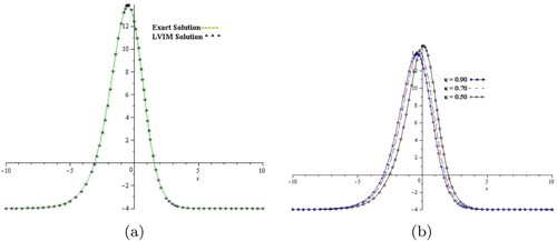
Figure 2. (a) The solution graph of exact and LVIM solution at $\kappa =1$ of Example 6.2 and (b) the solution-graph of Example 6.2 at different fractional-order κ. (a) Graph of LVIM and exact solutions for t = 0.1 and $\kappa =1$ for Example 6.2. (b) Graph of LVIM solutions for different value of κ for Example 6.2.

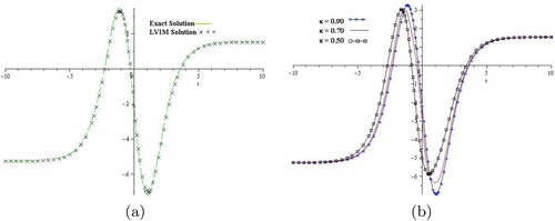
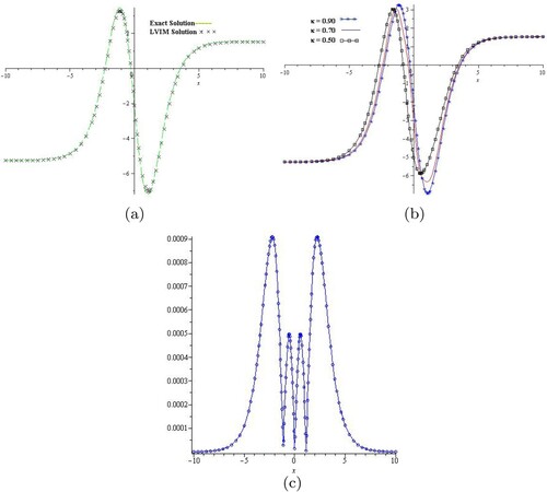
Figure 3. (a) The solution graph of exact and LVIM solution at $\kappa =1$ of example 6.3 and (b) the solution-graph of example 6.3 at different fractional-order κ. (a) Graph of LVIM and exact solutions for t = 0.1 and $\kappa =1$ for Example 6.3. (b) Graph of LVIM solutions for different value of κ for Example 6.3. (c) Error plot of Example 6.3 for $\kappa =1$.

Example 6.3

Consider the KS equation as defined by $\eta =1$ $\theta =0.5$ and $\omega =0$ [31,32]. (29) $\frac{{\mathrm{\partial }}^{\kappa }\mu }{\mathrm{\partial }{t}^{\kappa }}+\mu \frac{\mathrm{\partial }\mu }{\mathrm{\partial }x}+\eta \frac{{\mathrm{\partial }}^2\mu }{\mathrm{\partial }{x}^2}+\theta \frac{{\mathrm{\partial }}^3\mu }{\mathrm{\partial }{x}^3}+\omega \frac{{\mathrm{\partial }}^4\mu }{\mathrm{\partial }{x}^4}=0,$(29) with initial condition $\begin{array}{rl}{u}_0(x,0)& =-0.1858640755-2.973310349\tanh \\ & \left(\frac{\sqrt{418}}{38}x\right)+9.344689666{\tanh }^3\left(\frac{\sqrt{418}}{38}x\right),\end{array}$ Using LVIM on both sides equation (29(29) $\frac{{\mathrm{\partial }}^{\kappa }\mu }{\mathrm{\partial }{t}^{\kappa }}+\mu \frac{\mathrm{\partial }\mu }{\mathrm{\partial }x}+\eta \frac{{\mathrm{\partial }}^2\mu }{\mathrm{\partial }{x}^2}+\theta \frac{{\mathrm{\partial }}^3\mu }{\mathrm{\partial }{x}^3}+\omega \frac{{\mathrm{\partial }}^4\mu }{\mathrm{\partial }{x}^4}=0,$(29) ), we get (30) $\begin{array}{rl}{\mu }_{m+1}(x,t)& ={\text{£}}^{-1}\left[\frac{u_m(x,t)}{s}\right]+{\text{£}}^{-1}\left[\lambda \left(s\right)\left\{s^{\kappa }\frac{\mathrm{\partial }{\mu }_m}{\mathrm{\partial }s}\right.\right.\\ & +\left.\left.{\mu }_m\frac{\mathrm{\partial }{\mu }_m}{\mathrm{\partial }x}+\eta \frac{{\mathrm{\partial }}^2{\mu }_m}{\mathrm{\partial }{x}^2}+\theta \frac{{\mathrm{\partial }}^3{\mu }_m}{\mathrm{\partial }{x}^3}\right\}\right],\end{array}$(30) where $\lambda \left(s\right)$ is the Lagrange multiplier (31) $\begin{array}{rl}\lambda \left(s\right)& =\frac{-1}{s^{\kappa }},\\ {\mu }_{m+1}(x,t)& =u_m(x,t)-{\text{£}}^{-1}\left[\frac{1}{s^{\kappa }}\left\{s^{\kappa }\frac{\mathrm{\partial }{\mu }_m}{\mathrm{\partial }s}+{\mu }_m\frac{\mathrm{\partial }{\mu }_m}{\mathrm{\partial }x}\right.\right.\\ & +\left.\left.\eta \frac{{\mathrm{\partial }}^2{\mu }_m}{\mathrm{\partial }{x}^2}+\theta \frac{{\mathrm{\partial }}^3{\mu }_m}{\mathrm{\partial }{x}^3}\right\}\right].\end{array}$(31) Now take, $\begin{array}{rl}{u}_0(x,t)& =-0.1858640755-2.973310349\tanh \\ & \times \left(\frac{\sqrt{418}}{38}x\right)+9.344689666{\tanh }^3\left(\frac{\sqrt{418}}{38}x\right)\end{array}$ For m = 0 $\begin{array}{rl}{\mu }_1(x,t)& =u_0(x,t)-{\text{£}}^{-1}\left[\frac{1}{s^{\kappa }}\left\{s^{\kappa }\frac{\mathrm{\partial }{\mu }_0}{\mathrm{\partial }s}+{\mu }_0\frac{\mathrm{\partial }{\mu }_0}{\mathrm{\partial }x}\right.\right.\\ & +\left.\left.\eta \frac{{\mathrm{\partial }}^2{\mu }_0}{\mathrm{\partial }{x}^2}+\theta \frac{{\mathrm{\partial }}^3{\mu }_0}{\mathrm{\partial }{x}^3}\right\}\right],\\ u_1(x,t)& =-0.1858640755-2.973310349\tanh \\ & \times \left(\frac{\sqrt{418}}{38}x\right)+9.344689666{\tanh }^3\left(\frac{\sqrt{418}}{38}x\right)\\ & -\left[1.00\times {10}^{-17}\left\{8.00\times {10}^7{\cosh }^7\left(0.53x\right)\right.\right.\\ & -2.50\times {10}^{17}{\cosh }^5\left(0.53x\right)+2.80\times {10}^{17}\\ & \times {\cosh }^3\left(0.53x\right)-2.64\times {10}^9\sinh \left(0.53x\right)\\ & \times {\cosh }^6\left(0.53x\right)+6.29\times {10}^{18}\sinh \left(0.53x\right)\\ & \times {\cosh }^4\left(0.53x\right)-8.92\times {10}^{18}\sinh \left(0.53x\right)\\ & \times \left.\left.{\cosh }^2\left(0.53x\right)-3.59\times {10}^8\sinh \left(0.53x\right)\right\}\right]\\ & \times \frac{t^{\kappa }}{{\cosh }^7\left(0.53x\right)\mathrm{\Gamma }(\kappa +1)}.\end{array}$ For m = 1 $\begin{array}{rl}{\mu }_2(x,t)& =u_1(x,t)-{\text{£}}^{-1}\left[\frac{1}{s^{\kappa }}\left\{s^{\kappa }\frac{\mathrm{\partial }{\mu }_1}{\mathrm{\partial }s}+{\mu }_1\frac{\mathrm{\partial }{\mu }_1}{\mathrm{\partial }x}\right.\right.\\ & +\left.\left.\eta \frac{{\mathrm{\partial }}^2{\mu }_1}{\mathrm{\partial }{x}^2}+\theta \frac{{\mathrm{\partial }}^3{\mu }_1}{\mathrm{\partial }{x}^3}\right\}\right],\\ u_2(x,t)& =-0.1858640755-2.973310349\\ & \times \tanh \left(\frac{\sqrt{418}}{38}x\right)+9.344689666{\tanh }^3\\ & \times \left(\frac{\sqrt{418}}{38}x\right)\\ & -\left[1.00\times {10}^{-17}\left\{8.00\times {10}^7{\cosh }^7\left(0.53x\right)\right.\right.\\ & -2.50\times {10}^{17}{\cosh }^5\left(0.53x\right)+2.80\times {10}^{17}\\ & \times {\cosh }^3\left(0.53x\right)-2.64\times {10}^9\sinh \left(0.53x\right)\\ & \times {\cosh }^6\left(0.53x\right)+6.29\times {10}^{18}\sinh \left(0.53x\right)\\ & \times {\cosh }^4\left(0.53x\right)-8.92\times {10}^{18}\sinh \left(0.53x\right)\\ & \left.\left.\times {\cosh }^2\left(0.53x\right)-3.59\times {10}^8\sinh \left(0.53x\right)\right\}\right]\\ & \times \frac{t^{\kappa }}{{\cosh }^7\left(0.53x\right)\mathrm{\Gamma }(\kappa +1)}\\ & -[1.00\times {10}^{-27}\{-3.22\times {10}^{30}\sinh \left(0.53x\right)\\ & \times {\cosh }^6\left(0.53x\right)-1.80\times {10}^{20}\sinh \left(0.53x\right)\\ & +1.69\times {10}^{29}{\cosh }^7\left(0.53x\right)-2.40\times {10}^{29}\\ & \times {\cosh }^5\left(0.53x\right)+9.86\times {10}^{28}{\cosh }^3\left(0.53x\right)\\ & +6.28\times {10}^{3}0\sinh \left(0.53x\right)\\ & \times {\cosh }^4\left(0.53x\right)-3.59\times {10}^{30}\sinh \left(0.53x\right)\\ & \times {\cosh }^2\left(0.53x\right)-8.86\times {10}^{19}{\cosh }^{10}\left(0.53x\right)\\ & \times \sinh \left(0.53x\right)+4.09\times {10}^{29}{\cosh }^8\left(0.53x\right)\\ & \times \sinh \left(0.53x\right)+1.10\times {10}^9{\cosh }^{11}\left(0.53x\right)\\ & -2.97\times {10}^{28}\cosh \left(0.53x{)}^9\right\}]\\ & \times \frac{t^{2\kappa }}{{\cosh }^{11}\left(0.53x\right)\mathrm{\Gamma }(2\kappa +1)}.\end{array}$ For $m=2,3,\dots$ $\begin{array}{rl}{\mu }_{m+1}(x,t)& =u_m(x,t)-{\text{£}}^{-1}\left[\frac{1}{s^{\kappa }}\left[s^{\kappa }\frac{\mathrm{\partial }{\mu }_m}{\mathrm{\partial }s}+{\mu }_m\frac{\mathrm{\partial }{\mu }_m}{\mathrm{\partial }x}\right.\right.\\ & +\left.\left.\eta \frac{{\mathrm{\partial }}^2{\mu }_m}{\mathrm{\partial }{x}^2}+\theta \frac{{\mathrm{\partial }}^3{\mu }_m}{\mathrm{\partial }{x}^3}\right]\right].\end{array}$ The exact result is (32) $\begin{array}{rl}u(x,t)& =-\frac{0.5}{\varphi }+\frac{60}{19}\varphi (-38\theta {\varphi }^2+\eta )\tanh \left(\mathrm{\Phi }\right)\\ & +120\theta {\varphi }^3{\tanh }^3\left(\mathrm{\Phi }\right),\end{array}$(32) then $\mathrm{\Phi }=\varphi x+0.1t$ and $\varphi =0.5\sqrt{11\eta /19\theta }$, On the interval $[-1,1]$.

7. Conclusion

In the current research work, an extended Laplace variational iteration method is applied to obtain analytical solution of fractional Kuramoto–Sivashinsky equations. The proposed method is a simple and effective tool to solve fractional PDEs because it uses the Lagrange multiplier directly to solve fractional PDEs.

In conclusion, the present method have the straightforward implementation and small number of calculations and therefore can be implemented to other fractional-order PDE, that frequently arises in science and engineering.

Moreover, in future, the present method can be implemented to solve some important system of high non-linear fractional-order PDEs in applied science. In particular, the fractional-view analysis of some dynamical systems in economic, biology, physics, chemistry and engineering provide the best information about its physical, chemistry and engineering provide the best information about its physical behaviour. Therefore, in future, the proposed technique will be considered as an important tool to analyse and describe the fractional-order analysis of the important physical model.

Disclosure statement

No potential conflict of interest was reported by the author(s).

Additional information

Funding

The authors acknowledge the financial support provided by the Center of Excellence in Theoretical and Computational Science (TaCS-CoE), KMUTT.

References

- Yépez-Martínez H, Gómez-Aguilar F, Sosa IO, et al. The Feng's first integral method applied to the nonlinear mKdV space-time fractional partial differential equation. Revista mexicana de física. 2016;62:310–316.
- Baleanu D, Machado JA, Luo AC, editors. Fractional dynamics and control. Springer Science and Business Media; 2011.
- Magin Richard L. Fractional calculus in bioengineering. Chicago: Begell House Redding; 2006.
- Ellahi R, Alamri SZ, Basit A, et al. Effects of MHD and slip on heat transfer boundary layer flow over a moving plate based on specific entropy generation. J. Taibah Univ. Sci. 2018;12:476–482. doi: 10.1080/16583655.2018.1483795
- Li C, Qian D, Chen Y. On Riemann-Liouville and caputo derivatives. Discrete Dyn Nat Soc. 2011;2011:562494.
- Tenreiro Machado JA, Silva Manuel F, Barbosa Ramiro S, et al. Some applications of fractional calculus in engineering. Math Prob Eng. 2010;2010:639801. doi: 10.1155/2010/639801
- Gómez-Aguilar JF, Yépez-Martínez H, Escobar-Jiménez RF, et al. Series solution for the time-fractional coupled mKdV equation using the homotopy analysis method. Math Prob Eng. 2016;2016:7047126. doi: 10.1155/2016/7047126
- Atangana A, Gómez-Aguilar JF. Numerical approximation of Riemann-Liouville definition of fractional derivative: from Riemann-Liouville to Atangana-Baleanu. Numer Methods Partial Differ Equ. 2018;5:1502–1523. doi: 10.1002/num.22195
- Gómez-Aguilar JF, Atangana A. New insight in fractional differentiation: power, exponential decay and Mittag-Leffler laws and applications. Eur Phys J Plus. 2017;132:13. doi: 10.1140/epjp/i2017-11293-3
- Cuahutenango-Barro B, Taneco-Hernández MA, Gómez-Aguilar JF. On the solutions of fractional-time wave equation with memory effect involving operators with regular kernel. Chaos Solitons Fractals. 2018;115:283–299. doi: 10.1016/j.chaos.2018.09.002
- Gómez-Aguilar JF, Miranda-Hernández M, López-López MG, et al. Modeling and simulation of the fractional space-time diffusion equation. Commun Nonlinear Sci Numer Simul. 2016;30:115–127. doi: 10.1016/j.cnsns.2015.06.014
- Gómez-Aguilar JF. Space–time fractional diffusion equation using a derivative with nonsingular and regular kernel. Physica A. 2017;465:562–572. doi: 10.1016/j.physa.2016.08.072
- Saad KM, Gómez-Aguilar JF. Analysis of reaction–diffusion system via a new fractional derivative with non-singular kernel. Physica A. 2018;509:703–716. doi: 10.1016/j.physa.2018.05.137
- Rademacher JD, Wittenberg RW. Viscous shocks in the destabilized Kuramoto-Sivashinsky equation. J Comput Nonlinear Dyn. 2006;4:336–347. doi: 10.1115/1.2338656
- Zeeshan A, Hussain F, Ellahi R, et al. A study of gravitational and magnetic effects on coupled stress bi-phase liquid suspended with crystal and Hafnium particles down in steep channel. J Mol Liq. 2019;286:110898. doi: 10.1016/j.molliq.2019.110898
- Khan AA, Bukhari SR, Marin M. Effects of chemical reaction on third grade magnetohydrodynamics fluid flow under the influence of heat and mass transfer with variable reactive index. Heat Transf Res. 2019;50(11):1061–1080. doi: 10.1615/HeatTransRes.2018028397
- Prakash J, Tripathi D, Tiwari AK, et al. Peristaltic pumping of nanofluids through a tapered channel in a porous environment: applications in blood flow. Symmetry. 2019;7:868. doi: 10.3390/sym11070868
- Riaz A, Ellahi R, Bhatti MM. Study of heat and mass transfer in the Eyring-Powell model of fluid propagating peristaltically through a rectangular complaint channel. Heat Transf Res. 2019;50(16):1539–1560. doi: 10.1615/HeatTransRes.2019025622
- Conte R. Exact solutions of nonlinear partial differential equations by singularity analysis. In: Direct and inverse methods in nonlinear evolution equations. Berlin: Springer; 2003. p. 1–83.
- Kuramoto Y, Tsuzuki T. Persistent propagation of concentration waves in dissipative media far from thermal equilibrium. Prog Theor Phys. 1976;55:356–369. doi: 10.1143/PTP.55.356
- Tadmor E. The well-posedness of the Kuramoto–Sivashinsky equation. SIAM J Math Anal. 1986;17:884–893. doi: 10.1137/0517063
- Sivashinsky GI. Instabilities, pattern formation, and turbulence in flames. Annu Rev Fluid Mech. 1983;15:179–199. doi: 10.1146/annurev.fl.15.010183.001143
- Hooper AP, Grimshaw R. Nonlinear instability at the interface between two viscous fluids. Phys Fluids. 1985;28:37–45. doi: 10.1063/1.865160
- Khater AH, Temsah RS. Numerical solutions of the generalized Kuramoto–Sivashinsky equation by Chebyshev spectral collocation methods. Comput Math Appl. 2008;56:1465–1472. doi: 10.1016/j.camwa.2008.03.013
- Grimshaw R, Hooper AP. The non-existence of a certain class of travelling wave solutions of the Kuramoto-Sivashinsky equation. Physica D. 1991;50:231–238. doi: 10.1016/0167-2789(91)90177-B
- Liu X. Gevrey class regularity and approximate inertial manifolds for the Kuramoto-Sivashinsky equation. Physica D. 1991;50:135–151. doi: 10.1016/0167-2789(91)90085-N
- Xu Y, Shu CW. Local discontinuous Galerkin methods for the Kuramoto–Sivashinsky equations and the Ito-type coupled KdV equations. Comput Methods Appl Mech Eng. 2006;195:3430–3447. doi: 10.1016/j.cma.2005.06.021
- Abbasbandy S. Solitary wave solutions to the Kuramoto–Sivashinsky equation by means of the homotopy analysis method. Nonlinear Dyn. 2008;52:35–40. doi: 10.1007/s11071-007-9255-9
- Driscoll TA. A composite Runge–Kutta method for the spectral solution of semilinear PDEs. J Comput Phys. 2002;182:357–367. doi: 10.1006/jcph.2002.7127
- Singh BK, Arora G, Kumar P. A note on solving the fourth-order Kuramoto-Sivashinsky equation by the compact finite difference scheme. Ain Shams Eng J. 2016;9(4):1581–1589. doi: 10.1016/j.asej.2016.11.008
- Lakestani M, Dehghan M. Numerical solutions of the generalized Kuramoto–Sivashinsky equation using B-spline functions. Appl Math Model. 2012;36:605–617. doi: 10.1016/j.apm.2011.07.028
- Uddin M, Haq S. A mesh-free numerical method for solution of the family of Kuramoto–Sivashinsky equations. Appl Math Comput. 2009;212:458–469.
- Acan O, Keskin Y. Approximate solution of Kuramoto–Sivashinsky equation using reduced differential transform method. In: AIP Conference Proceedings. AIP Publishing; 2015. p. 1648.
- Lai H, Ma C. Lattice Boltzmann method for the generalized Kuramoto–Sivashinsky equation. Physica A. 2009;388:1405–1412. doi: 10.1016/j.physa.2009.01.005
- Kudryashov NA. Quasi-exact solutions of the dissipative Kuramoto–Sivashinsky equation. Appl Math Comput. 2013;219:9213–9218.
- Rezazadeh H, Ziabarya BP. Sub-equation method for the conformable fractional generalized Kuramoto Sivashinsky equation. Comput Res Prog Appl Sci Eng. 2016;2:106–109.
- Wazzan L. A modified tanh–coth method for solving the general Burgers–Fisher and the Kuramoto–Sivashinsky equations. Commun Nonlinear Sci Numer Simul. 2009;14:2642–2652. doi: 10.1016/j.cnsns.2008.08.004
- Inokuti M, Sekine H, Mura T. General use of the Lagrange multiplier in nonlinear mathematical physics. Variational Method Mech Solids. 1978;33:156–162.
- He JH. Approximate analytical solution for seepage flow with fractional derivatives in porous media. Comput Methods Appl Mech Eng. 1998;167:57–68. doi: 10.1016/S0045-7825(98)00108-X
- He JH. Variational iteration method–a kind of non-linear analytical technique: some examples. Int J Non-Linear Mech. 1999;34:699–708. doi: 10.1016/S0020-7462(98)00048-1
- Hristov J. An exercise with the He's variation iteration method to a fractional Bernoulli equation arising in a transient conduction with a non-linear boundary heat flux. Int Rev Chem Eng. 2012;4:489–497.
- Liu CF, Kong SS, Yuan SJ. Reconstructive schemes for variational iteration method within Yang-Laplace transform with application to fractal heat conduction problem. Therm Sci. 2013;17:715–721. doi: 10.2298/TSCI120826075L
- Wu GC, Lee EW. Fractional variational iteration method and its application. Phys Lett A. 2010;374:2506–2509. doi: 10.1016/j.physleta.2010.04.034
- Hesameddini E, Latifizadeh H. Reconstruction of variational iteration algorithms using the Laplace transform. Int J Nonlinear Sci Numer Simul. 2009;10:1377–1382.
- Khuri SA, Sayfy A. A Laplace variational iteration strategy for the solution of differential equations. Appl Math Lett. 2012;25:2298–2305. doi: 10.1016/j.aml.2012.06.020
- Wu GC, Baleanu D. Variational iteration method for fractional calculus-a universal approach by Laplace transform. Adv Differ Equ. 2013;2013:18. doi: 10.1186/1687-1847-2013-18
- Jafari H, Jassim HK. Approximate solution for nonlinear gas dynamic and coupled KdV equations involving local fractional operator. J Zankoy Sulaimani–Part A. 2016;18:127–132. doi: 10.17656/jzs.10456
- Ahmed HF, Bahgat MS, Zaki M. Numerical approaches to system of fractional partial differential equations. J Egypt Math Soc. 2017;25:141–150. doi: 10.1016/j.joems.2016.12.004
- Borisut P, Kumam P, Ahmed I, et al. Nonlinear Caputo Fractional Derivative with Nonlocal Riemann-Liouville Fractional Integral Condition Via Fixed Point Theorems. Symmetry. 2019;11(6):829. doi: 10.3390/sym11060829
- Akgül A, Bonyah E. Reproducing kernel Hilbert space method for the solutions of generalized Kuramoto–Sivashinsky equation. J Taibah Univ Sci. 2019;13:661–690. doi: 10.1080/16583655.2019.1618547
- Shah R, Khan H, Arif M, et al. Application of Laplace–Adomian decomposition method for the analytical solution of third-order dispersive fractional partial differential equations. Entropy. 2019;21:335. doi: 10.3390/e21040335
- Mahmood S, Shah R, Arif M. Laplace adomian decomposition method for multi dimensional time fractional model of Navier-Stokes equation. Symmetry. 2019;11:149. doi: 10.3390/sym11020149
- Rudolf H. Applications of fractional calculus in physics. Singapore: World Scientific; 2000.
- Podlubny I. Fractional differential equations: an introduction to fractional derivatives, fractional differential equations, to methods of their solution and some of their applications. San Diego: Elsevier; 1998.
- Miller KS, Ross B. An introduction to the fractional calculus and fractional differential equations. New York: John Wiley & Sons; 1993.
- Ghaneai H, Hosseini MM. Variational iteration method with an auxiliary parameter for solving wave-like and heat-like equations in large domains. Comput Math Appl. 2015;69:363–373. doi: 10.1016/j.camwa.2014.11.007