Minimizing the expected search time of finding the hidden object by maximizing the discount effort reward search

Abstract

A new search technique is developed to locate the hidden target (object) in one of the N-disjoint regions that are not identical. The lost object follows a bivariate distribution. Minimizing the search effort with discount reward has been applied instead of reducing the expected search time. Moreover, the minimum number of searchers is determined in order to minimize the total expected cost. Assuming the object's position has a Circular Normal distribution, the Kuhn–Tucker necessary conditions are implemented to get the optimum search plan.

Keywords:

• Search theory
• coordinated search technique
• circular normal distribution

Mathematics Subject Classifications:

• 37A50
• 60K30
• 90B40

1. Introduction

The detection of explosives in places where they are likely to be present in the shortest possible time will prevent many innocent victims. Minimizing the time and the effort to detect one of the explosive needs to increase the number of searchers and the coordination process among them. The case of the randomly located object with a known distribution on the real line has been discussed by Reyniers [1,2]. She considered two unit speeds searchers aim to find this object in the shortest possible time. In addition, Mohamed et al. [3,4] studied this problem for the hidden object which has a known distribution in an open area.

On the other hand, for a stochastically moving object, El-Hadidy and Abou-Gabal [5] and El-Hadidy and Alzulaibani [6,7] used a linear coordinated search technique to present a finite search plan which minimizes the first collision time expected value between one of the searchers and the stochastically moving object. Moreover, this technique is applied by using the Bayesian approach (see, e.g. [8–11]). Earlier, many interesting methods to track the stochastically moving object have been presented by Dai et al. [12] and Deilami et al. [13]. Besides that, Mohamed et al. [14,15], Mohamed and El-Hadidy [16], Mohamed and El-Hadidy [17], Beltagy and El-Hadidy [18], Abou-Gabal and El-Hadidy [19], Mohamed et al. [20], Kassem and El-Hadidy [21], El-Hadidy and El-Bagoury [22], El-Hadidy [23–31], El-Hadidy and Alzulaibani [6,7], and El-Hadidy et al. [32] provided many different mathematical treatments of this issue in both cases stochastically moving and hidden objects.

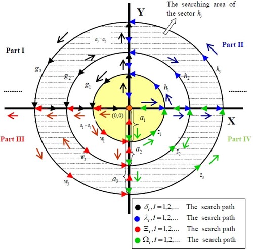
This paper aims to coordinate the search technique that allows the M-searchers $S_j,j=1,2,\dots ,M$ (where M is an even number), start together and searching for a hidden object from the centre of each region $R_{\ell },\ell =1,2,\dots ,N$  (a point $(0,0)$) , as shown in Figure 1 (the search path in the region $R_{\ell }$ which has 4-unit speed searchers). The purpose is to find the minimum expected value of the detection time by achieving the optimal search plan after applying the discount effort reward function which has been applied before in  [25].

Figure 1. The search path in $R_{\ell }$ with 4-searchers.

In this work, Section 2 explains the problem and presents the expected reward cost of detection. In Section 3, the optimal search policy that minimizes the expected reward cost of detection is presented after considering the Circular Normal distribution of the object's position. A discussion of the results and future works is presented in the conclusion part.

2. Problem formulation

The mathematical model of this problem is formulated by considering the discounted search effort reward. This model gives the expected value of the discounted effort reward for detection in one of N-disjoint and not identical regions $R_{\ell },\ell =1,2,\dots ,N.$

2.1. The searching process

The search space: The space is divided into N-disjoint and not identical regions $R_{\ell },\ell =1,2,\dots ,N$. Each region has two roads intersected at the centre of this region. These roads divide the region into four identical parts. The two roads are considered as x and y axes (see Figure 1). Here, the report for the object position is given at $(0,0)$.

The object: The object is randomly located in one of these regions with symmetric distribution about $(0,0)$.

The means of search: Let M searchers start the searching process for the object from the $(0,0)$ in each region. Each region has an even number of searchers. The searchers go along the two axes ($+ve$ and $-ve$ parts) with equal speeds. The sectors and its tracks are searched with regular speed. The searchers return to $(0,0)$ and still searching until the object detected.

2.2. 4-Coordinated search technique in the region $R_{\ell }$

Let the position of the object in $R_{\ell }$ be defined by the two independent random variables $(X,Y)$. The surface of $R_{\ell }$ is a “ Standard Euclidean 2-space E”, with points $(x,y)$. In $R_{\ell }$, we have four searchers, $S_{k\ell },k=1,2,3,4,$ each searcher of them is always searching one part from the four parts (see Figure 1). We will divide the region into many sectors, as shown in Figure 1.

2.2.1. The Searching path

To find the object, the searchers $S_{k\ell },k=1,2,3,4,$ follow ${\delta }_{\ell },$ ${\lambda }_{\ell },{\mathrm{\Xi }}_{\ell }$ and ${\mathrm{\Omega }}_{\ell }$ (the search paths), respectively. The first search path ${\delta }_{1\ell }$ of $S_{1\ell }$ is defined as follows:

1. Begin at the point $(0,0)$ and go along the right part of the y-axis ($+ve$ part) as far as $a_{1\ell }.$

2. Look for the object in $g_{1\ell }$ and its track.

3. When $S_{1\ell }$ reaches the point $(-a_{1\ell },0),$ $S_{1\ell }$ will return to the origin through $-ve$ part of the x-axis.

In addition, one can define the second search path ${\delta }_{2\ell }$ of $S_{1\ell }$ as in the above steps ($\left(i\right)$, $\left(ii\right)$ and $\left(iii\right)$), where $S_{1\ell }$ goes a distance $a_{2\ell }$ to search the sector $g_{2\ell }$ and its track, etc. Thus, ${\delta }_{\ell }$ of $S_{1\ell }$ is completely defined by a sequence $\{{\delta }_{i\ell },i\ge 0\}$. The first search path ${\lambda }_{1\ell }$ of $S_{2\ell }$ is defined as follows:

1. Begin at $(0,0)$ and go along the left part of the y-axis ($-ve$ part) as far as $a_{1\ell }.$

2. Search the sector $h_{1\ell }$ and its track.

3. When $S_{2\ell }$ reaches the point $(0,a_{1\ell }),$ $S_{2\ell }$ will return to the origin through $-ve$ part of the x-axis.

And, ${\lambda }_{2\ell }$ ( the second search path) of $S_{2\ell }$ is defined as in the above steps from (a) to (c), where $S_{2\ell }$ goes a distance $a_{2\ell }$ to search $h_{2\ell }$ and its track, etc. Thus, ${\lambda }_{\ell }$ of $S_{2\ell }$ is completely defined by the sequence $\{{\lambda }_{i\ell },i\ge 0\}$.

Also, by considering the searchers' movement on the sectors and tracks done in anticlockwise, then the search paths of $S_{3\ell }$, $S_{4\ell }$ are $\{{\mathrm{\Xi }}_{i\ell },i\ge 0\}$ and $\{{\mathrm{\Omega }}_{i\ell },i\ge 0\},$ respectively, where $S_{3\ell }$, $S_{4\ell }$ search the parts III and IV.

Each searcher goes along the x-axis with speed v = 1 and searches the circles, the tracks with regular speed ${\text{β}}_{\ell }$. The time that the searcher takes it through going on the x-axis will add to the time of the searching process (sectors and its tracks searching time).

Let the surface of $R_{\ell }$ be a “ Standard Euclidean 2-space E” and the object position has the probability density function $f(x,y)$. Also, let $t_{ik\ell },i=1,2,\dots ,$ k = 1, 2, 3, 4, be the time that the searchers $S_{k\ell },k=1,2,3,4$ take it in $\{{\delta }_{i\ell },i\ge 0\},\{{\lambda }_{i\ell },i\ge 0\},\{{\mathrm{\Xi }}_{i\ell },i\ge 0\}$ and $\{{\mathrm{\Omega }}_{i\ell },i\ge 0\}$ in the four parts to $(0,0),$ where any track i has a width $a_{i\ell }-a_{(i-1)\ell }$. They go on the y-axis and x-axis from the origin before searching the sectors. In addition, they return after finishing the searching process with equal speeds v = 1 to $(0,0)$. Then, the time of going through the y-axis is equal to the distances which done. They are searching $g_{i\ell },h_{i\ell },w_{i\ell },z_{i\ell },i=1,2,\dots$ (sectors and tracks) with ${\text{β}}_{\ell }.$ Then, the searching time is equal to ${\tau }_{i\ell }=2\pi /{\omega }_{i\ell }$, where ${\tau }_{i\ell }$ is the time league and ${\omega }_{i\ell }$ is called angular velocity. The searching time ${\tau }_{i\ell }$ depends on ${\omega }_{i\ell }$ which depends on the radius $a_{i\ell }$ and the time of detection $t\left({\phi }_{\ell }\right)$

We choose the discounted effort function as an exponential function $D_{\ell }\left(i\right)=d_{\ell }^i,0<d_{\ell }<1$, that will reduce the possible rewards at the revolution number i (see [25]). The adjust parameter $d_{\ell }$ gives permission to make the decision indirectly, and this helps the searcher to take appropriate actions in the future.

Theorem 2.1

The expected reward cost of detection for the lost object is given by

(1) $\begin{array}{rl}E\left(t\right({\phi }_{\ell }\left)\right)& =\sum _{i=1}^{\mathrm{\infty }}\left[\left(8a_{i\ell }+\frac{2\pi }{{\omega }_{i\ell }}\right)\cdot 4d_{\ell }^i\right.\\ & \left.\cdot \left[\sum _{s=i}^{\mathrm{\infty }}\sum _{u=1}^n{\int }_{a_{(s-1)\ell }}^{a_{s\ell }}{\int }_{{\theta }_{(u-1)\ell }}^{{\theta }_{u\ell }}{g}_{\ell }(r_{\ell },{\theta }_{\ell })r_{\ell }\mathrm{d}{r}_{\ell }\mathrm{d}{\theta }_{\ell }\right]\right].\end{array}$(1)

Proof.

The object may be in one of the four parts in $R_{\ell }$. Thus, more appropriate formulas for the expected time are available. This leads to the following:

If the object is located at any point on the track of $g_{1\ell },$ then $t_{2\ell }=2a_{1\ell }+\pi /2{\omega }_1$.

If the object is located at any point on the track of $g_{2\ell },$ then $t_{2\ell }=2(a_{1\ell }+a_2)+\left(\pi /2\right)(1/{\omega }_1+1/{\omega }_2)$.

If the object is located at any point on the track of $g_{3\ell },$ then $t_{2\ell }=2(a_{1\ell }+a_2+a_3)+\left(\pi /2\right)(1/{\omega }_1+1/{\omega }_2+1/{\omega }_3)$, etc.

If the object is located at any point on the track of $h_{1\ell }$, then $t_{1\ell }=a_{1\ell }+\frac{1}{4}\left(2\pi /{\omega }_{1\ell }\right)+a_{1\ell }=2a_{1\ell }+\pi /2{\omega }_{1\ell }$.

If the object is located at any point on the track of $h_{2\ell }$, then $t_{1\ell }=2(a_{1\ell }+a_{2\ell })+\left(\pi /2\right)(1/{\omega }_{1\ell }+1/{\omega }_{2\ell })$.

If the object is located at any point on the track of $h_{3\ell }$, then $t_{1\ell }=2(a_{1\ell }+a_{2\ell }+a_{3\ell })+\left(\pi /2\right)(1/{\omega }_{1\ell }+(1/{\omega }_{2\ell })+1/{\omega }_{3\ell })$, etc.

If the object is located at any point on the track of $w_{1\ell },$ then $t_{1\ell }=a_{1\ell }+\frac{1}{4}\left(2\pi /{\omega }_1\right)+a_{1\ell }=2a_{1\ell }+\left(\pi /2{\omega }_{1\ell }\right)$.

If the object is located at any point on the track of $w_{2\ell },$ then $t_{1\ell }=2(a_{1\ell }+a_{2\ell })+\left(\pi /2\right)(1/{\omega }_{1\ell }+1/{\omega }_2)$.

If the object is located at any point on the track of $w_{3\ell },$ then $t_{1\ell }=2(a_{1\ell }+a_{2\ell }+a_{3\ell })+\left(\pi /2\right)(1/{\omega }_{1\ell }+1/{\omega }_{2\ell }+1/{\omega }_{3\ell })$, and etc.

If the object is located at any point on the track of $z_{1\ell },$ then $t_{2\ell }=2a_{1\ell }+\pi /2{\omega }_{1\ell }$.

If the object is located at any point on the track of $z_{2\ell },$ then $t_{2\ell }=2(a_{1\ell }+a_{2\ell })+\left(\pi /2\right)(1/{\omega }_{1\ell }+1/{\omega }_{2\ell })$.

If the object is located at any point on the track of $z_{3\ell },$ then $t_{2\ell }=2(a_{1\ell }+a_{2\ell }+a_{3\ell })+\left(\pi /2\right)(1/{\omega }_{1\ell }+1/{\omega }_{2\ell }+1/{\omega }_{3\ell })$, etc.

Each sector is divided into equal small sectors $l_{u\ell },u=1,2,\dots ,n$, where these sectors make a set of equal cones. As in Figure 2, these cones have the same vertex $(0,0)$. Thus, each searcher can cover a track with width $a_{i\ell }-a_{(i-1)\ell }$ which has equal small areas of cones in the track number i. These cones are determined by a set of lines with equations $x=m_{u\ell }y=\tan {\theta }_{\ell }$ y, where ${\theta }_{\ell }={\theta }_{u\ell }-{\theta }_{(u-1)\ell },$ $u=1,2,\dots ,n$. These equations give a range of equal small spaces to equalize the searching process. Applying the polar coordinates with $x=r_{\ell }\cos {\theta }_{\ell }$ and $y=r_{\ell }\sin {\theta }_{\ell }$, $r_{\ell }:a_{(i-1)\ell }⟶a_{i\ell }$, $i=1,2,3,\dots ,$ and ${\theta }_{\ell }:{\theta }_{(u-1)\ell }⟶{\theta }_{u\ell }$, $u=1,2,3,\dots ,n,$ where $a_{0\ell }=r_{0\ell }=0$ and ${\theta }_{0\ell }=0$ to evaluate the expected searching time to detect the object. The searching process is performed in the anticlockwise direction.

Figure 2. The small search area in $R_{\ell }$ which is made by small sectors $l_{u\ell },u=1,2,\dots ,n,$ which made by the searchers inside the circles with radiuses $a_{i\ell },i=1,2,3,\dots$

By using our assumptions where the object has symmetric distribution and applying the discounted effort reward function in each revolution, we have $\begin{array}{rl}E\left(t\right({\phi }_{\ell }\left)\right)& =\left(2a_{1\ell }+\frac{\pi }{2{\omega }_{1\ell }}\right)\cdot d_{\ell }^1\\ & \cdot \left[{\int }_0^{a_{1\ell }}{\int }_0^{{\theta }_{1\ell }}{g}_{\ell }(r_{\ell },{\theta }_{\ell })r_{\ell }\mathrm{d}{r}_{\ell }\mathrm{d}{\theta }_{\ell }+\cdots \right.\\ & \left.+{\int }_0^{a_{1\ell }}{\int }_{{\theta }_{(n-1)\ell }}^{{\theta }_{n\ell }}{g}_{\ell }(r_{\ell },{\theta }_{\ell })r_{\ell }\mathrm{d}{r}_{\ell }\mathrm{d}{\theta }_{\ell }\right]\\ & +\left(2(a_{1\ell }+a_{2\ell })+\frac{\pi }{2}\left(\frac{1}{{\omega }_{1\ell }}+\frac{1}{{\omega }_{2\ell }}\right)\right)\\ & \cdot (d_{\ell }^1+d_{\ell }^2)\\ & \times \left[{\int }_{a_{1\ell }}^{a_{2\ell }}{\int }_0^{{\theta }_{1\ell }}{g}_{\ell }(r_{\ell },{\theta }_{\ell })r_{\ell }\mathrm{d}{r}_{\ell }\mathrm{d}{\theta }_{\ell }+\cdots \right.\\ & \left.+{\int }_{a_{1\ell }}^{a_{2\ell }}{\int }_{{\theta }_{(n-1)\ell }}^{{\theta }_{n\ell }}{g}_{\ell }(r_{\ell },{\theta }_{\ell })r_{\ell }\mathrm{d}{r}_{\ell }d{\theta }_{\ell }\right]\\ & +\left(2(a_{1\ell }+a_{2\ell }+a_{3\ell })+\frac{\pi }{2}\right.\\ & \left.\times \left(\frac{1}{{\omega }_{1\ell }}+\frac{1}{{\omega }_{2\ell }}+\frac{1}{{\omega }_{3\ell }}\right)\right)\cdot (d_{\ell }^1+d_{\ell }^2+d_{\ell }^3)\\ & \times \left[{\int }_{a_{2\ell }}^{a_{3\ell }}{\int }_0^{{\theta }_{1\ell }}{g}_{\ell }(r_{\ell },{\theta }_{\ell })r_{\ell }\mathrm{d}{r}_{\ell }\mathrm{d}{\theta }_{\ell }+\cdot \right.\\ & \left.s+{\int }_{a_{2\ell }}^{a_{3\ell }}{\int }_{{\theta }_{(n-1)\ell }}^{{\theta }_{n\ell }}{g}_{\ell }(r_{\ell },{\theta }_{\ell })r_{\ell }\mathrm{d}{r}_{\ell }\mathrm{d}{\theta }_{\ell }\right]\\ & +\cdots \\ & +\left(2a_{1\ell }+\frac{\pi }{2{\omega }_{1\ell }}\right)\cdot d_{\ell }^1\\ & \times \left[{\int }_0^{a_{1\ell }}{\int }_0^{{\theta }_{1\ell }}{g}_{\ell }(r_{\ell },{\theta }_{\ell })r_{\ell }\mathrm{d}{r}_{\ell }\mathrm{d}{\theta }_{\ell }+\cdots \right.\\ & \left.+{\int }_0^{a_{1\ell }}{\int }_{{\theta }_{(n-1)\ell }}^{{\theta }_{n\ell }}{g}_{\ell }(r_{\ell },{\theta }_{\ell })r_{\ell }\mathrm{d}{r}_{\ell }\mathrm{d}{\theta }_{\ell }\right]\\ & +\left(2(a_{1\ell }+a_{2\ell })+\frac{\pi }{2}\left(\frac{1}{{\omega }_{1\ell }}+\frac{1}{{\omega }_{2\ell }}\right)\right)\end{array}$ $\begin{array}{r}\times (d_{\ell }^1+d_{\ell }^2)\\ & \times \left[{\int }_{a_{1\ell }}^{a_{2\ell }}{\int }_0^{{\theta }_{1\ell }}{g}_{\ell }(r_{\ell },{\theta }_{\ell })r_{\ell }\mathrm{d}{r}_{\ell }\mathrm{d}{\theta }_{\ell }+\cdots \right.\\ & \left.+{\int }_{a_{1\ell }}^{a_2}{\int }_{{\theta }_{n-1}}^{{\theta }_n}{g}_{\ell }(r_{\ell },{\theta }_{\ell })r_{\ell }\mathrm{d}{r}_{\ell }\mathrm{d}{\theta }_{\ell }\right]\\ & +\left(2(a_{1\ell }+a_{2\ell }+a_{3\ell })+\frac{\pi }{2}\right.\\ & \left.\times \left(\frac{1}{{\omega }_{1\ell }}+\frac{1}{{\omega }_{2\ell }}+\frac{1}{{\omega }_{3\ell }}\right)\right)\cdot (d_{\ell }^1+d_{\ell }^2+d_{\ell }^3)\\ & \times \left[{\int }_{a_{2\ell }}^{a_{3\ell }}{\int }_0^{{\theta }_{1\ell }}{g}_{\ell }(r_{\ell },{\theta }_{\ell })r_{\ell }\mathrm{d}{r}_{\ell }\mathrm{d}{\theta }_{\ell }+\cdots \right.\\ & \left.+{\int }_{a_{2\ell }}^{a_{3\ell }}{\int }_{{\theta }_{(n-1)\ell }}^{{\theta }_{n\ell }}{g}_{\ell }(r_{\ell },{\theta }_{\ell })r_{\ell }\mathrm{d}{r}_{\ell }\mathrm{d}{\theta }_{\ell }\right]\\ & +\cdots \\ & +\left(2a_{1\ell }+\frac{\pi }{2{\omega }_{1\ell }}\right)\cdot d_{\ell }^1\\ & \times \left[{\int }_0^{a_{1\ell }}{\int }_0^{{\theta }_{1\ell }}{g}_{\ell }(r_{\ell },{\theta }_{\ell })r_{\ell }\mathrm{d}{r}_{\ell }\mathrm{d}{\theta }_{\ell }+\cdots \right.\\ & \left.+{\int }_0^{a_{1\ell }}{\int }_{{\theta }_{(n-1)\ell }}^{{\theta }_{n\ell }}{g}_{\ell }(r_{\ell },{\theta }_{\ell })r_{\ell }\mathrm{d}{r}_{\ell }\mathrm{d}{\theta }_{\ell }\right]\\ & +\left(2(a_{1\ell }+a_{2\ell })+\frac{\pi }{2}\left(\frac{1}{{\omega }_{1\ell }}+\frac{1}{{\omega }_{2\ell }}\right)\right)\\ & \times (d_{\ell }^1+d_{\ell }^2)\\ & \times \left[{\int }_{a_{1\ell }}^{a_{2\ell }}{\int }_0^{{\theta }_{1\ell }}{g}_{\ell }(r_{\ell },{\theta }_{\ell })r_{\ell }\mathrm{d}{r}_{\ell }\mathrm{d}{\theta }_{\ell }+\cdots \right.\\ & \left.+{\int }_{a_{1\ell }}^{a_{2\ell }}{\int }_{{\theta }_{(n-1)\ell }}^{{\theta }_{n\ell }}{g}_{\ell }(r_{\ell },{\theta }_{\ell })r_{\ell }\mathrm{d}{r}_{\ell }\mathrm{d}{\theta }_{\ell }\right]\\ & +\left(2(a_{1\ell }+a_{2\ell }+a_{3\ell })+\frac{\pi }{2}\right.\\ & \left.\times \left(\frac{1}{{\omega }_{1\ell }}+\frac{1}{{\omega }_{2\ell }}+\frac{1}{{\omega }_{3\ell }}\right)\right)\cdot (d_{\ell }^1+d_{\ell }^2+d_{\ell }^3)\end{array}$ $\begin{array}{r}\times \left[{\int }_{a_{2\ell }}^{a_{3\ell }}{\int }_0^{{\theta }_{1\ell }}{g}_{\ell }(r_{\ell },{\theta }_{\ell })r_{\ell }\mathrm{d}{r}_{\ell }\mathrm{d}{\theta }_{\ell }+\cdots \right.\\ & \left.+{\int }_{a_{2\ell }}^{a_{3\ell }}{\int }_{{\theta }_{(n-1)\ell }}^{{\theta }_{n\ell }}{g}_{\ell }(r_{\ell },{\theta }_{\ell })r_{\ell }\mathrm{d}{r}_{\ell }\mathrm{d}{\theta }_{\ell }\right]\\ & +\cdots \\ & +\left(2a_{1\ell }+\frac{\pi }{2{\omega }_{1\ell }}\right)\cdot d_{\ell }^1\\ & \times \left[{\int }_0^{a_{1\ell }}{\int }_0^{{\theta }_{1\ell }}{g}_{\ell }(r_{\ell },{\theta }_{\ell })r_{\ell }\mathrm{d}{r}_{\ell }\mathrm{d}{\theta }_{\ell }+\cdots \right.\\ & \left.+{\int }_0^{a_{1\ell }}{\int }_{{\theta }_{(n-1)\ell }}^{{\theta }_{n\ell }}{g}_{\ell }(r_{\ell },{\theta }_{\ell })r_{\ell }\mathrm{d}{r}_{\ell }\mathrm{d}{\theta }_{\ell }\right]\\ & +\left(2(a_{1\ell }+a_{2\ell })+\frac{\pi }{2}\left(\frac{1}{{\omega }_{1\ell }}+\frac{1}{{\omega }_{2\ell }}\right)\right)\\ & \times (d_{\ell }^1+d_{\ell }^2)\\ & \times \left[{\int }_{a_{1\ell }}^{a_{2\ell }}{\int }_0^{{\theta }_{1\ell }}{g}_{\ell }(r_{\ell },{\theta }_{\ell })r_{\ell }\mathrm{d}{r}_{\ell }\mathrm{d}{\theta }_{\ell }+\cdots \right.\\ & \left.+{\int }_{a_{1\ell }}^{a_{2\ell }}{\int }_{{\theta }_{(n-1)\ell }}^{{\theta }_{n\ell }}{g}_{\ell }(r_{\ell },{\theta }_{\ell })r_{\ell }\mathrm{d}{r}_{\ell }\mathrm{d}{\theta }_{\ell }\right]\\ & +\left(2(a_{1\ell }+a_{2\ell }+a_{3\ell })+\frac{\pi }{2}\right.\\ & \left.\times \left(\frac{1}{{\omega }_{1\ell }}+\frac{1}{{\omega }_{2\ell }}+\frac{1}{{\omega }_{3\ell }}\right)\right)\cdot (d_{\ell }^1+d_{\ell }^2+d_{\ell }^3)\\ & \times \left[{\int }_{a_{2\ell }}^{a_{3\ell }}{\int }_0^{{\theta }_{1\ell }}{g}_{\ell }(r_{\ell },{\theta }_{\ell })r_{\ell }\mathrm{d}{r}_{\ell }\mathrm{d}{\theta }_{\ell }+\cdots \right.\\ & \left.+{\int }_{a_{2\ell }}^{a_{3\ell }}{\int }_{{\theta }_{(n-1)\ell }}^{{\theta }_{n\ell }}{g}_{\ell }(r_{\ell },{\theta }_{\ell })r_{\ell }\mathrm{d}{r}_{\ell }\mathrm{d}{\theta }_{\ell }\right]+\cdots ,\end{array}$ etc., then $\begin{array}{rl}E\left(t\right({\phi }_{\ell }\left)\right)& =4\left[2a_{1\ell }+\frac{\pi }{2{\omega }_{1\ell }}\right]\cdot d_{\ell }^1\\ & \times \left[\sum _{u=1}^n{\int }_0^{a_{1\ell }}{\int }_{{\theta }_{(u-1)\ell }}^{{\theta }_{u\ell }}{g}_{\ell }(r_{\ell },{\theta }_{\ell })r_{\ell }\mathrm{d}{r}_{\ell }\mathrm{d}{\theta }_{\ell }\right]\\ & +4\left[2(a_{1\ell }+a_{2\ell })+\frac{\pi }{2}\left(\frac{1}{{\omega }_{1\ell }}+\frac{1}{{\omega }_{2\ell }}\right)\right]\\ & \times (d_{\ell }^1+d_{\ell }^2)\\ & \times \left[\sum _{u=1}^n{\int }_{a_{1\ell }}^{a_{2\ell }}{\int }_{{\theta }_{(u-1)\ell }}^{{\theta }_{u\ell }}{g}_{\ell }(r_{\ell },{\theta }_{\ell })r_{\ell }\mathrm{d}{r}_{\ell }d{\theta }_{\ell }\right]\\ & +4\left[2(a_{1\ell }+a_{2\ell }+a_{3\ell })+\frac{\pi }{2}\right.\\ & \left.\times \left(\frac{1}{{\omega }_{1\ell }}+\frac{1}{{\omega }_{2\ell }}+\frac{1}{{\omega }_{3\ell }}\right)\right]\cdot (d_{\ell }^1+d_{\ell }^2+d_{\ell }^3)\\ & \times \left[\sum _{u=1}^n{\int }_{a_{2\ell }}^{a_{3\ell }}{\int }_{{\theta }_{(u-1)\ell }}^{{\theta }_{u\ell }}{g}_{\ell }(r_{\ell },{\theta }_{\ell })r_{\ell }\mathrm{d}{r}_{\ell }\mathrm{d}{\theta }_{\ell }\right]\\ & +\cdots \\ & =\left(8a_{1\ell }+\frac{2\pi }{{\omega }_{1\ell }}\right)\cdot 4d_{\ell }^1\\ & \times \left[\sum _{u=1}^n{\int }_0^{a_{1\ell }}{\int }_{{\theta }_{(u-1)\ell }}^{{\theta }_{u\ell }}{g}_{\ell }(r_{\ell },{\theta }_{\ell })r_{\ell }\mathrm{d}{r}_{\ell }\mathrm{d}{\theta }_{\ell }\right.\\ & +\sum _{u=1}^n{\int }_{a_{1\ell }}^{a_{2\ell }}{\int }_{{\theta }_{(u-1)\ell }}^{{\theta }_{u\ell }}{g}_{\ell }(r_{\ell },{\theta }_{\ell })r_{\ell }\mathrm{d}{r}_{\ell }\mathrm{d}{\theta }_{\ell }\\ & \left.+\sum _{u=1}^n{\int }_{a_{2\ell }}^{a_{3\ell }}{\int }_{{\theta }_{(u-1)\ell }}^{{\theta }_{u\ell }}{g}_{\ell }(r_{\ell },{\theta }_{\ell })r_{\ell }\mathrm{d}{r}_{\ell }\mathrm{d}{\theta }_{\ell }+\cdots \right]\\ & +\left(8a_{2\ell }+\frac{2\pi }{{\omega }_{2\ell }}\right)\cdot 4d_{\ell }^2\\ & \times \left[\sum _{u=1}^n{\int }_{a_{1\ell }}^{a_{2\ell }}{\int }_{{\theta }_{(u-1)\ell }}^{{\theta }_{u\ell }}{g}_{\ell }(r_{\ell },{\theta }_{\ell })r_{\ell }\mathrm{d}{r}_{\ell }\mathrm{d}{\theta }_{\ell }\right.\\ & +\sum _{u=1}^n{\int }_{a_{2\ell }}^{a_{3\ell }}{\int }_{{\theta }_{(u-1)\ell }}^{{\theta }_{u\ell }}{g}_{\ell }(r_{\ell },{\theta }_{\ell })r_{\ell }\mathrm{d}{r}_{\ell }\mathrm{d}{\theta }_{\ell }\\ & \left.+\sum _{u=1}^n{\int }_{a_{3\ell }}^{a_{4\ell }}{\int }_{{\theta }_{(u-1)\ell }}^{{\theta }_{u\ell }}{g}_{\ell }(r_{\ell },{\theta }_{\ell })r_{\ell }\mathrm{d}{r}_{\ell }\mathrm{d}{\theta }_{\ell }+\cdots \right]\\ & +\left(8a_{3\ell }+\frac{2\pi }{{\omega }_{3\ell }}\right)\cdot 4d_{\ell }^3\\ & \times \left[\sum _{u=1}^n{\int }_{a_{2\ell }}^{a_{3\ell }}{\int }_{{\theta }_{(u-1)\ell }}^{{\theta }_{u\ell }}{g}_{\ell }(r_{\ell },{\theta }_{\ell })r_{\ell }\mathrm{d}{r}_{\ell }\mathrm{d}{\theta }_{\ell }\right.\\ & \left.+\sum _{u=1}^n{\int }_{a_{3\ell }}^{a_{4\ell }}{\int }_{{\theta }_{(u-1)\ell }}^{{\theta }_{u\ell }}{g}_{\ell }(r_{\ell },{\theta }_{\ell })r_{\ell }\mathrm{d}{r}_{\ell }\mathrm{d}{\theta }_{\ell }+\cdots \right]\\ & +\cdots \\ & =\sum _{i=1}^{\mathrm{\infty }}\left[\left(8a_{i\ell }+\frac{2\pi }{{\omega }_{i\ell }}\right)\cdot 4d_{\ell }^i\right.\\ & \left.\times \left[\sum _{s=i}^{\mathrm{\infty }}\sum _{u=1}^n{\int }_{a_{(s-1)\ell }}^{a_{s\ell }}{\int }_{{\theta }_{(u-1)\ell }}^{{\theta }_{u\ell }}{g}_{\ell }(r_{\ell },{\theta }_{\ell })r_{\ell }\mathrm{d}{r}_{\ell }d{\theta }_{\ell }\right]\right].\end{array}$

Corollary 2.2

In the case of two searchers, one of them searches the sectors in the right part of the y-axis and the other searches the sectors in the left part. In addition, the object has symmetric distribution and $d_{\ell }^i=\frac{1}{2}$. Then, the expected value of the time for the searchers to return to the origin after the object detection is (2) $\begin{array}{rl}E\left(t\right({\phi }_{\ell }\left)\right)& =\sum _{i=1}^{\mathrm{\infty }}\left[\left(4a_{i\ell }+\frac{\pi }{{\omega }_{i\ell }}\right)\right.\\ & \left.\cdot \left[\sum _{s=i}^{\mathrm{\infty }}\sum _{u=1}^n{\int }_{a_{(s-1)\ell }}^{a_{s\ell }}{\int }_{{\theta }_{(u-1)\ell }}^{{\theta }_{u\ell }}{g}_{\ell }(r_{\ell },{\theta }_{\ell })r_{\ell }\mathrm{d}{r}_{\ell }\mathrm{d}{\theta }_{\ell }\right]\right].\end{array}$(2) It is the same result which has been obtained before in [3] when $d_{\ell }^i\ne \frac{1}{2},i=1,2,\dots ,0<d_{\ell }<1$; we found that the expected reward cost of detection for the two searchers to return to $(0,0)$ after the object has been detected as in (2(2) $\begin{array}{rl}E\left(t\right({\phi }_{\ell }\left)\right)& =\sum _{i=1}^{\mathrm{\infty }}\left[\left(4a_{i\ell }+\frac{\pi }{{\omega }_{i\ell }}\right)\right.\\ & \left.\cdot \left[\sum _{s=i}^{\mathrm{\infty }}\sum _{u=1}^n{\int }_{a_{(s-1)\ell }}^{a_{s\ell }}{\int }_{{\theta }_{(u-1)\ell }}^{{\theta }_{u\ell }}{g}_{\ell }(r_{\ell },{\theta }_{\ell })r_{\ell }\mathrm{d}{r}_{\ell }\mathrm{d}{\theta }_{\ell }\right]\right].\end{array}$(2) ) will become (3) $\begin{array}{rl}E\left(t\right({\phi }_{\ell }\left)\right)& =\sum _{i=1}^{\mathrm{\infty }}\left[\left(4a_{i\ell }+\frac{\pi }{{\omega }_{i\ell }}\right)\cdot 2d_{\ell }^i\right.\\ & \left.\cdot \left[\sum _{s=i}^{\mathrm{\infty }}\sum _{u=1}^n{\int }_{a_{(s-1)\ell }}^{a_{s\ell }}{\int }_{{\theta }_{(u-1)\ell }}^{{\theta }_{u\ell }}{g}_{\ell }(r_{\ell },{\theta }_{\ell })r_{\ell }\mathrm{d}{r}_{\ell }\mathrm{d}{\theta }_{\ell }\right]\right],\end{array}$(3) which is less than the expected value of the time in (2(2) $\begin{array}{rl}E\left(t\right({\phi }_{\ell }\left)\right)& =\sum _{i=1}^{\mathrm{\infty }}\left[\left(4a_{i\ell }+\frac{\pi }{{\omega }_{i\ell }}\right)\right.\\ & \left.\cdot \left[\sum _{s=i}^{\mathrm{\infty }}\sum _{u=1}^n{\int }_{a_{(s-1)\ell }}^{a_{s\ell }}{\int }_{{\theta }_{(u-1)\ell }}^{{\theta }_{u\ell }}{g}_{\ell }(r_{\ell },{\theta }_{\ell })r_{\ell }\mathrm{d}{r}_{\ell }\mathrm{d}{\theta }_{\ell }\right]\right].\end{array}$(2) ). Also, we can notice that the expected value of the time in the case of $q_{\ell }$ searchers, where $q_{\ell }$ is even number, is smaller than the expected value of $(q_{\ell }-2)$ searchers; this leads to the following:

Theorem 2.3

For any even number $q_{\ell }$ of searchers in one of the non-identical N-regions, where $\sum _{\ell =1}^N$ $q_{\ell }=M,$ the total expected reward cost of detection is given by

(4) $\begin{array}{rl}E\left(t\right(\phi \left)\right)& =\sum _{\ell =1}^N\left(\sum _{i=1}^{\mathrm{\infty }}\left[\left(2q_{\ell }{a}_{i\ell }+\frac{q_{\ell }\pi }{2{\omega }_{i\ell }}\right)\cdot q_{\ell }{d}_{\ell }^i\right.\right.\\ & \left.\left.\cdot \left[\sum _{s=i}^{\mathrm{\infty }}\sum _{u=1}^n{\int }_{a_{(s-1)\ell }}^{a_{s\ell }}{\int }_{{\theta }_{(u-1)\ell }}^{{\theta }_{u\ell }}{g}_{\ell }(r_{\ell },{\theta }_{\ell })r_{\ell }\mathrm{d}{r}_{\ell }\mathrm{d}{\theta }_{\ell }\right]\right]\right).\end{array}$(4)

Proof.

By the same method that prove Theorem 2.1 we can prove this theorem.

Corollary 2.4

If the width is fixed $($i.e. $a_{i\ell }-a_{(i-1)\ell }=a),$ then $a_1=a,$ $a_2=2a,$ $a_3=3a,\dots ,$ and if $q_{\ell }=q,{\theta }_{u\ell }-{\theta }_{(u-1)\ell }=\theta$ then in (4(4) $\begin{array}{rl}E\left(t\right(\phi \left)\right)& =\sum _{\ell =1}^N\left(\sum _{i=1}^{\mathrm{\infty }}\left[\left(2q_{\ell }{a}_{i\ell }+\frac{q_{\ell }\pi }{2{\omega }_{i\ell }}\right)\cdot q_{\ell }{d}_{\ell }^i\right.\right.\\ & \left.\left.\cdot \left[\sum _{s=i}^{\mathrm{\infty }}\sum _{u=1}^n{\int }_{a_{(s-1)\ell }}^{a_{s\ell }}{\int }_{{\theta }_{(u-1)\ell }}^{{\theta }_{u\ell }}{g}_{\ell }(r_{\ell },{\theta }_{\ell })r_{\ell }\mathrm{d}{r}_{\ell }\mathrm{d}{\theta }_{\ell }\right]\right]\right).\end{array}$(4) ) we have $\begin{array}{rl}E\left(t\right(\phi \left)\right)& =\sum _{i=1}^{\mathrm{\infty }}\left[\left(2ia+\frac{\pi }{2i\omega }\right)\cdot N^3{q}^2{d}^i\right.\\ & \left.\cdot \left[\sum _{s=i}^{\mathrm{\infty }}\sum _{u=1}^n{\int }_{(s-1)a}^{sa}{\int }_{(u-1)\theta }^{u\theta }g(r,\theta )r\mathrm{d}r\mathrm{d}\theta \right]\right].\end{array}$

The above result shows that this technique is more suitable to detect an important object (like a bomb or a person in a wilderness area) by using $q_{\ell }$ searchers.

3. Optimal search plan

Since the main contribution of this technique is to minimize the expected cost of detection, then we need to get the optimal search plan ${\phi }^{\ast }\in \mathrm{\Phi },$ which give $E\left(t\right({\phi }^{\ast }\left)\right)=inf\left\{E\right(t\left(\phi \right)),\phi \in \mathrm{\Phi }\},$ where ${\phi }^{\ast }$ depend on the optimal paths ${\delta }^{\ast }=\{{\delta }_{i\ell }^{\ast },i\ge 0,\ell =1,2,\dots ,N\},{\lambda }^{\ast }=\{{\lambda }_{i\ell }^{\ast },i\ge 0,\ell =1,2,\dots ,N\},{\mathrm{\Xi }}^{\ast }=\{{\mathrm{\Xi }}_{i\ell }^{\ast },i\ge 0,\ell =1,2,\dots ,N\}$ and ${\mathrm{\Omega }}^{\ast }=\{{\mathrm{\Omega }}_{i\ell }^{\ast },i\ge 0,\ell =1,2,\dots ,N\}$. Rather than finding the optimal sequence $\{a_i^{\ast }-a_{i-1}^{\ast };i\ge 0\}$ (optimal values of the turning points $a_i$ for a given initial object distribution), which gives the optimal paths ${\delta }^{\ast },{\lambda }^{\ast },$ ${\mathrm{\Xi }}^{\ast }$ and ${\mathrm{\Omega }}^{\ast },$ we need to maximize the discounted effort reward $d_{\ell }^i,\ell =1,2,\dots ,N,$ or minimize $(1-d_{\ell }^i)$ to get $d_{\ell }^{i\ast }$ for each revolution$i,i=1,2,3,\dots$. The probability of the object in each region will be affected by the number of searchers. But, the increasing searchers' number will increase the searching cost. Thus, we also need to obtain the optimal number of searchers in each region $q_{\ell },\ell =1,2,\dots ,N;$ this will reduce the total cost.

Really, we face a difficult optimization problem because our problem has an infinite number of variables; that is, $a_{\ell }=\{a_{i\ell }-a_{(i-1)\ell };i\ge 0,\ell =1,2,\dots ,N\},$ which depends on the object distribution F. In addition, we have $({\omega }_{i\ell }{)}^{\mathrm{\prime }}s$ are considering an infinite number of variables where $({\omega }_{i\ell }{)}^{\mathrm{\prime }}s$ also depend on $(a_{i\ell }{)}^{\mathrm{\prime }}s$, $v_i={\omega }_i{a}_i$ and speed $v_i$ is “regular speed” on any circle. Therefore, if we take $v_i=\text{β}=$constant, we can obtain the optimal values of “ angular velocity” in any circle from ${\omega }_{i\ell }^{\ast }=\text{β}/a_{i\ell }^{\ast }$, $i=1,2,3,\dots$. Let us assume, from now on, that the object distribution be known with expected value $A\left(F\right)<\mathrm{\infty }$.

It is clear that, if $\acute{Q}$ $\subseteq Q$ (the class of all possible search plans) for which there is only one element and if $a_{\ell }^{\ast }$ is an optimal search path on the x-axis, then all the optimal search paths will be ${\delta }^{\ast },{\lambda }^{\ast },$ ${\mathrm{\Xi }}^{\ast }$ and ${\mathrm{\Omega }}^{\ast }$ which belongs to $\acute{Q}$. Consequently, besides the condition $A\left(F\right)<\mathrm{\infty },$ we can assume that for the necessary condition on the known object's distribution, there exists a search path ${\delta }^{\ast }=\{{\delta }_{i\ell }^{\ast },i\ge 0,\ell =1,2,\dots ,N\},{\lambda }^{\ast }=\{{\lambda }_{i\ell }^{\ast },i\ge 0,\ell =1,2,\dots ,N\},{\mathrm{\Xi }}^{\ast }=\{{\mathrm{\Xi }}_{i\ell }^{\ast },i\ge 0,\ell =1,2,\dots ,N\}$ and ${\mathrm{\Omega }}^{\ast }=\{{\mathrm{\Omega }}_{i\ell }^{\ast },i\ge 0,\ell =1,2,\dots ,N\}$ from class Q such that $D({\delta }^{\ast },{\lambda }^{\ast },{\mathrm{\Xi }}^{\ast },{\mathrm{\Omega }}^{\ast },D_{\ell }^{\ast };F)=m$.

Theorem 3.1

If $A\left(F\right)<\mathrm{\infty }$ and $D_{\ell }\left(i\right)=d_{\ell }^i,0<d_{\ell }<1$ in each region $R_{\ell },$ $\ell =1,2,\dots ,N,$ then there exists a search path from class Q with finite expected reward cost, which can also lead to $m<\mathrm{\infty }$ [33].

After proving that objective function (4(4) $\begin{array}{rl}E\left(t\right(\phi \left)\right)& =\sum _{\ell =1}^N\left(\sum _{i=1}^{\mathrm{\infty }}\left[\left(2q_{\ell }{a}_{i\ell }+\frac{q_{\ell }\pi }{2{\omega }_{i\ell }}\right)\cdot q_{\ell }{d}_{\ell }^i\right.\right.\\ & \left.\left.\cdot \left[\sum _{s=i}^{\mathrm{\infty }}\sum _{u=1}^n{\int }_{a_{(s-1)\ell }}^{a_{s\ell }}{\int }_{{\theta }_{(u-1)\ell }}^{{\theta }_{u\ell }}{g}_{\ell }(r_{\ell },{\theta }_{\ell })r_{\ell }\mathrm{d}{r}_{\ell }\mathrm{d}{\theta }_{\ell }\right]\right]\right).\end{array}$(4) ) is convex, we will use the Kuhn–Tucker conditions to obtain these optimal values which minimizes $E\left(t\right(\phi \left)\right)$. Hence, we will obtain the following non-linear programming problem (NLP(1)): $\begin{array}{rl}\mathbf{\text{NLP(1):}}& \\ \underset{a_{i\ell },q_{\ell }}{min}\underset{d_{\ell }^i}{max}& E\left(t\right(\phi \left)\right)\\ \text{subject to}& 0\le \sum _{i=1}^{\mathrm{\infty }}\sum _{\ell =1}^N\sum _{u=1}^n{\int }_{a_{(i-1)\ell }}^{a_{i\ell }}{\int }_{{\theta }_{(u-1)\ell }}^{{\theta }_{u\ell }}{g}_{\ell }\\ & (r_{\ell },{\theta }_{\ell })r_{\ell }\mathrm{d}{r}_{\ell }\mathrm{d}{\theta }_{\ell }\le 1,\\ & a_{i\ell }-a_{(i-1)\ell }>0,q_{\ell }>0,\\ & 0<d_{\ell }^i<1,i=2,3,\dots ,\mathrm{\infty },\\ \mathrm{w}\mathrm{h}\mathrm{e}\mathrm{r}\mathrm{e}E\left(t\right(\phi \left)\right)& =\sum _{\ell =1}^N\left(\sum _{i=1}^{\mathrm{\infty }}\left[\left(2q_{\ell }{a}_{i\ell }+\frac{q_{\ell }\pi }{2{\omega }_{i\ell }}\right)\cdot q_{\ell }{d}_{\ell }^i\right.\right.\\ & \cdot \left[\sum _{s=i}^{\mathrm{\infty }}\sum _{u=1}^n{\int }_{a_{(s-1)\ell }}^{a_{s\ell }}{\int }_{{\theta }_{(u-1)\ell }}^{{\theta }_{u\ell }}{g}_{\ell }(r_{\ell },{\theta }_{\ell })\right.\\ & \left.\left.\left.\phantom{\sum _{s=i}^{\mathrm{\infty }}}{r}_{\ell }\mathrm{d}{r}_{\ell }d{\theta }_{\ell }\right]\right]\right).\end{array}$

This is equivalent to the following: $\begin{array}{rl}\mathbf{\text{NLP(2):}}& \\ \underset{a_{i\ell },q_{\ell },d_{\ell }^i}{min}& \sum _{\ell =1}^N\left(\sum _{i=1}^{\mathrm{\infty }}\left[\left(2q_{\ell }{a}_{i\ell }+\frac{q_{\ell }\pi }{2{\omega }_{i\ell }}\right)\cdot q_{\ell }(1-d_{\ell }^i)\right.\right.\\ & \cdot \left[\sum _{s=i}^{\mathrm{\infty }}\sum _{u=1}^n{\int }_{a_{(s-1)\ell }}^{a_{s\ell }}{\int }_{{\theta }_{(u-1)\ell }}^{{\theta }_{u\ell }}{g}_{\ell }(r_{\ell },{\theta }_{\ell })\right.\\ & \left.\left.\left.\phantom{\sum _{s=i}^{\mathrm{\infty }}}{r}_{\ell }\mathrm{d}{r}_{\ell }\mathrm{d}{\theta }_{\ell }\right]\right]\right)\\ \text{subject to}& \sum _{i=1}^{\mathrm{\infty }}\sum _{\ell =1}^N\sum _{u=1}^n{\int }_{a_{(i-1)\ell }}^{a_{i\ell }}{\int }_{{\theta }_{(u-1)\ell }}^{{\theta }_{u\ell }}{g}_{\ell }(r_{\ell },{\theta }_{\ell })r_{\ell }\mathrm{d}{r}_{\ell }\\ & \times \mathrm{d}{\theta }_{\ell }-1\le 0,a_{(i-1)\ell }-a_{i\ell }<0,\\ & -q_{\ell }<0,d_{\ell }^i-1<0,i=2,3,\dots ,\mathrm{\infty }.\end{array}$

From the Kuhn–Tucker conditions, we obtain $\begin{array}{rl}\frac{\mathrm{\partial }E\left(t\right(\phi \left)\right)}{\mathrm{\partial }{a}_{i\ell }}+\sum _{\chi =1}^4{U}_{i\chi }\frac{\mathrm{\partial }{G}_i(a_{i\ell },q_{\ell },d_{\ell }^i)}{\mathrm{\partial }{a}_{i\ell }}& =0,\\ \frac{\mathrm{\partial }E\left(t\right(\phi \left)\right)}{\mathrm{\partial }{q}_{\ell }}+\sum _{\chi =1}^4{U}_{i\chi }\frac{\mathrm{\partial }{G}_i(a_{i\ell },q_{\ell },d_{\ell }^i)}{\mathrm{\partial }{q}_{\ell }}& =0,\\ \frac{\mathrm{\partial }E\left(t\right(\phi \left)\right)}{\mathrm{\partial }{d}_{\ell }^i}+\sum _{\chi =1}^4{U}_{i\chi }\frac{\mathrm{\partial }{G}_i(a_{i\ell },q_{\ell },d_{\ell }^i)}{\mathrm{\partial }{d}_{\ell }^i}& =0,\\ \mathrm{\partial }{G}_i(a_{i\ell },q_{\ell },d_{\ell }^i)& \le 0,\\ U_{i\chi }\mathrm{\partial }{G}_i(a_{i\ell },q_{\ell },d_{\ell }^i)& =0,\\ U_{i\chi }& \ge 0.\end{array}$

Since ${\omega }_{i\ell }=\text{β}/a_{i\ell }$, we have (5) $\begin{array}{rl}& \sum _{\ell =1}^N\sum _{i=1}^{\mathrm{\infty }}\left(\left(2q_{\ell }-\frac{2{\acute{\omega }}_{i\ell }{q}_{\ell }\pi }{4{\omega }_{i\ell }^2}\right)\cdot q_{\ell }(1-d_{\ell }^i)\right)\\ & \cdot \left[\sum _{s=i}^{\mathrm{\infty }}\sum _{u=1}^n{\int }_{a_{(s-1)\ell }}^{a_{s\ell }}{\int }_{{\theta }_{(u-1)\ell }}^{{\theta }_{u\ell }}{g}_{\ell }(r_{\ell },{\theta }_{\ell })r_{\ell }\mathrm{d}{r}_{\ell }\mathrm{d}{\theta }_{\ell }\right]\\ & +\sum _{\ell =1}^N\sum _{i=1}^{\mathrm{\infty }}\left(\left(2q_{\ell }{a}_{i\ell }+\frac{q_{\ell }\pi }{2{\omega }_{i\ell }}\right)\cdot q_{\ell }(1-d_{\ell }^i)\right)\\ & \cdot \left[\sum _{s=i}^{\mathrm{\infty }}\sum _{u=1}^n\frac{\mathrm{\partial }}{\mathrm{\partial }{a}_{i\ell }}{\int }_{a_{(s-1)\ell }}^{a_{s\ell }}{\int }_{{\theta }_{(u-1)\ell }}^{{\theta }_{u\ell }}{g}_{\ell }(r_{\ell },{\theta }_{\ell })r_{\ell }\mathrm{d}{r}_{\ell }\mathrm{d}{\theta }_{\ell }\right]\\ & +U_{i1}\sum _{i=1}^{\mathrm{\infty }}\sum _{\ell =1}^N\sum _{u=1}^n\frac{\mathrm{\partial }}{\mathrm{\partial }{a}_{i\ell }}{\int }_{a_{(i-1)\ell }}^{a_{i\ell }}{\int }_{{\theta }_{(u-1)\ell }}^{{\theta }_{u\ell }}{g}_{\ell }(r_{\ell },{\theta }_{\ell })r_{\ell }\mathrm{d}{r}_{\ell }\mathrm{d}{\theta }_{\ell }\\ & +U_{i2}(-1)=0,\end{array}$(5) (6) $\begin{array}{rl}& \sum _{\ell =1}^N\sum _{i=1}^{\mathrm{\infty }}\left(\left(2a_{i\ell }+\frac{\pi }{2{\omega }_{i\ell }}\right)\cdot q_{\ell }(1-d_{\ell }^i)\right)\\ & \cdot \left[\sum _{s=i}^{\mathrm{\infty }}\sum _{u=1}^n{\int }_{a_{(s-1)\ell }}^{a_{s\ell }}{\int }_{{\theta }_{(u-1)\ell }}^{{\theta }_{u\ell }}{g}_{\ell }(r_{\ell },{\theta }_{\ell })r_{\ell }\mathrm{d}{r}_{\ell }\mathrm{d}{\theta }_{\ell }\right]\\ & +\sum _{\ell =1}^N\sum _{i=1}^{\mathrm{\infty }}\left(\left(2q_{\ell }{a}_{i\ell }+\frac{q_{\ell }\pi }{2{\omega }_{i\ell }}\right)\cdot (1-d_{\ell }^i)\right)\\ & \cdot \left[\sum _{s=i}^{\mathrm{\infty }}\sum _{u=1}^n{\int }_{a_{(s-1)\ell }}^{a_{s\ell }}{\int }_{{\theta }_{(u-1)\ell }}^{{\theta }_{u\ell }}{g}_{\ell }(r_{\ell },{\theta }_{\ell })r_{\ell }\mathrm{d}{r}_{\ell }\mathrm{d}{\theta }_{\ell }\right]\\ & +U_{i3}(-1)=0,\end{array}$(6) (7) $\begin{array}{rl}& -\sum _{\ell =1}^N\sum _{i=1}^{\mathrm{\infty }}\left(2q_{\ell }{a}_{i\ell }+\frac{q_{\ell }\pi }{2{\omega }_{i\ell }}\right)\cdot q_{\ell }\\ & \cdot \left[\sum _{s=i}^{\mathrm{\infty }}\sum _{u=1}^n{\int }_{a_{(s-1)\ell }}^{a_{s\ell }}{\int }_{{\theta }_{(u-1)\ell }}^{{\theta }_{u\ell }}{g}_{\ell }(r_{\ell },{\theta }_{\ell })r_{\ell }\mathrm{d}{r}_{\ell }\mathrm{d}{\theta }_{\ell }\right]\\ & +U_{i4}\left(1\right)=0,\end{array}$(7) (8) $\begin{array}{rl}& U_{i1}\left\{\sum _{i=1}^{\mathrm{\infty }}\sum _{\ell =1}^N\sum _{u=1}^n{\int }_{a_{(i-1)\ell }}^{a_{i\ell }}{\int }_{{\theta }_{(u-1)\ell }}^{{\theta }_{u\ell }}{g}_{\ell }(r_{\ell },{\theta }_{\ell })r_{\ell }\mathrm{d}{r}_{\ell }\mathrm{d}{\theta }_{\ell }-1\right\}\\ & =0,\end{array}$(8) (9) $\begin{array}{rl}& U_{i2}\{a_{(i-1)\ell }-a_{i\ell }\}=0,\end{array}$(9) (10) $\begin{array}{rl}& U_{i3}\{-q_{\ell }\}=0,\end{array}$(10) (11) $\begin{array}{rl}& U_{i4}\{d_{\ell }^i-1\}=0.\end{array}$(11)

Many cases have been found to solve Equations (5(5) $\begin{array}{rl}& \sum _{\ell =1}^N\sum _{i=1}^{\mathrm{\infty }}\left(\left(2q_{\ell }-\frac{2{\acute{\omega }}_{i\ell }{q}_{\ell }\pi }{4{\omega }_{i\ell }^2}\right)\cdot q_{\ell }(1-d_{\ell }^i)\right)\\ & \cdot \left[\sum _{s=i}^{\mathrm{\infty }}\sum _{u=1}^n{\int }_{a_{(s-1)\ell }}^{a_{s\ell }}{\int }_{{\theta }_{(u-1)\ell }}^{{\theta }_{u\ell }}{g}_{\ell }(r_{\ell },{\theta }_{\ell })r_{\ell }\mathrm{d}{r}_{\ell }\mathrm{d}{\theta }_{\ell }\right]\\ & +\sum _{\ell =1}^N\sum _{i=1}^{\mathrm{\infty }}\left(\left(2q_{\ell }{a}_{i\ell }+\frac{q_{\ell }\pi }{2{\omega }_{i\ell }}\right)\cdot q_{\ell }(1-d_{\ell }^i)\right)\\ & \cdot \left[\sum _{s=i}^{\mathrm{\infty }}\sum _{u=1}^n\frac{\mathrm{\partial }}{\mathrm{\partial }{a}_{i\ell }}{\int }_{a_{(s-1)\ell }}^{a_{s\ell }}{\int }_{{\theta }_{(u-1)\ell }}^{{\theta }_{u\ell }}{g}_{\ell }(r_{\ell },{\theta }_{\ell })r_{\ell }\mathrm{d}{r}_{\ell }\mathrm{d}{\theta }_{\ell }\right]\\ & +U_{i1}\sum _{i=1}^{\mathrm{\infty }}\sum _{\ell =1}^N\sum _{u=1}^n\frac{\mathrm{\partial }}{\mathrm{\partial }{a}_{i\ell }}{\int }_{a_{(i-1)\ell }}^{a_{i\ell }}{\int }_{{\theta }_{(u-1)\ell }}^{{\theta }_{u\ell }}{g}_{\ell }(r_{\ell },{\theta }_{\ell })r_{\ell }\mathrm{d}{r}_{\ell }\mathrm{d}{\theta }_{\ell }\\ & +U_{i2}(-1)=0,\end{array}$(5) )–(11(11) $\begin{array}{rl}& U_{i4}\{d_{\ell }^i-1\}=0.\end{array}$(11) ) as follows:

1. ($\mathrm{♠}$) $U_{i\chi }=0,\chi =1,2,3,4$;

2. ($▴$) $U_{i\chi }>0,\chi =1,2,3,4$;

3. ($▾$) $U_{i\mathrm{\wp }}>0,\mathrm{\wp }\in \{1,2,3,4\}$ and $U_{i\chi }=0,\chi =1,2,3,4,\mathrm{\wp }\ne \chi$;

4. (♣) $U_{i\mathrm{\wp }}>0,U_{i\hslash }>0,\mathrm{\wp },\hslash \in \{1,2,3,4\}$ and $U_{i\chi }=0,\chi =1,2,3,4,\mathrm{\wp }\ne \hslash \ne \chi$; and

5. ($⧫$) $U_{i\mathrm{\wp }}>0,U_{i\hslash }>0,U_{i\yen }>0,\mathrm{\wp },\hslash ,\yen \in \{1,2,3,4\}$ and $U_{i\chi }=0,\chi =1,2,3,4,\mathrm{\wp }\ne \hslash \ne \yen \ne \chi$.

Definition 3.1

In the revolution number $i,i=1,2,3,\dots ,$ and region $\ell ,\ell =1,2,\dots ,N,$ the optimal values $a_{i\ell }^{\ast },d_{\ell }^{i\ast },q_{\ell }^{\ast }\in \mathbb{R},$ where $0<d_{\ell }<1$ and $q_{\ell }^{\ast }=\lfloor q_{\ell }^{\ast }\rfloor$ (the optimal small integer value of $q_{\ell }$), are said to be optimal solutions of the above NLP, if there exist $\delta (a_{i\ell }^{\ast },d_{\ell }^{i\ast },q_{\ell }^{\ast })\le \delta (a_{i\ell },d_{\ell }^i,q_{\ell }),$ $\lambda (a_{i\ell }^{\ast },d_{\ell }^{i\ast },q_{\ell }^{\ast })\le \lambda (a_{i\ell },d_{\ell }^i,q_{\ell }),$ $\mathrm{\Xi }(a_{i\ell }^{\ast },d_{\ell }^{i\ast },q_{\ell }^{\ast })\le \mathrm{\Xi }(a_{i\ell },d_{\ell }^i,q_{\ell })$ and $\mathrm{\Omega }(a_{i\ell }^{\ast },d_{\ell }^{i\ast },q_{\ell }^{\ast })\le \mathrm{\Omega }(a_{i\ell },d_{\ell }^i,q_{\ell })$ for all $a_{i\ell },d_{\ell }^i,q_{\ell }\in \mathbb{R}$.

Since $\sum _{i=1}^{\mathrm{\infty }}\sum _{\ell =1}^N\sum _{u=1}^n{\int }_{a_{(i-1)\ell }}^{a_{i\ell }}{\int }_{{\theta }_{(u-1)\ell }}^{{\theta }_{u\ell }}{g}_{\ell }(r_{\ell },{\theta }_{\ell })r_{\ell }\mathrm{d}{r}_{\ell }\mathrm{d}{\theta }_{\ell }\le 1,$ $a_{i\ell }-a_{(i-1)\ell }>0,$ $q_{\ell }>0$ and $d_{\ell }^i>0,i=1,2,3,\dots ,\mathrm{\infty },$ then the optimal solution will be given after using the case (♠). Thus, we have the following system of equations: (12) $\begin{array}{rl}& \sum _{\ell =1}^N\sum _{i=1}^{\mathrm{\infty }}\left(\left(2q_{\ell }-\frac{2{\acute{\omega }}_{i\ell }{q}_{\ell }\pi }{4{\omega }_{i\ell }^2}\right)\cdot q_{\ell }(1-d_{\ell }^i)\right)\\ & \cdot \left[\sum _{s=i}^{\mathrm{\infty }}\sum _{u=1}^n{\int }_{a_{(s-1)\ell }}^{a_{s\ell }}{\int }_{{\theta }_{(u-1)\ell }}^{{\theta }_{u\ell }}{g}_{\ell }(r_{\ell },{\theta }_{\ell })r_{\ell }\mathrm{d}{r}_{\ell }\mathrm{d}{\theta }_{\ell }\right]\\ & +\sum _{\ell =1}^N\sum _{i=1}^{\mathrm{\infty }}\left(\left(2q_{\ell }{a}_{i\ell }+\frac{q_{\ell }\pi }{2{\omega }_{i\ell }}\right)\cdot q_{\ell }(1-d_{\ell }^i)\right)\\ & \cdot \left[\sum _{s=i}^{\mathrm{\infty }}\sum _{u=1}^n\frac{\mathrm{\partial }}{\mathrm{\partial }{a}_{i\ell }}{\int }_{a_{(s-1)\ell }}^{a_{s\ell }}{\int }_{{\theta }_{(u-1)\ell }}^{{\theta }_{u\ell }}{g}_{\ell }(r_{\ell },{\theta }_{\ell })r_{\ell }\mathrm{d}{r}_{\ell }d{\theta }_{\ell }\right]\\ & =0,\end{array}$(12) (13) $\begin{array}{rl}& \sum _{\ell =1}^N\sum _{i=1}^{\mathrm{\infty }}\left(\left(2a_{i\ell }+\frac{\pi }{2{\omega }_{i\ell }}\right)\cdot q_{\ell }(1-d_{\ell }^i)\right)\\ & \cdot \left[\sum _{s=i}^{\mathrm{\infty }}\sum _{u=1}^n{\int }_{a_{(s-1)\ell }}^{a_{s\ell }}{\int }_{{\theta }_{(u-1)\ell }}^{{\theta }_{u\ell }}{g}_{\ell }(r_{\ell },{\theta }_{\ell })r_{\ell }\mathrm{d}{r}_{\ell }\mathrm{d}{\theta }_{\ell }\right]\\ & +\sum _{\ell =1}^N\sum _{i=1}^{\mathrm{\infty }}\left(\left(2q_{\ell }{a}_{i\ell }+\frac{q_{\ell }\pi }{2{\omega }_{i\ell }}\right)\cdot (1-d_{\ell }^i)\right)\\ & \cdot \left[\sum _{s=i}^{\mathrm{\infty }}\sum _{u=1}^n{\int }_{a_{(s-1)\ell }}^{a_{s\ell }}{\int }_{{\theta }_{(u-1)\ell }}^{{\theta }_{u\ell }}{g}_{\ell }(r_{\ell },{\theta }_{\ell })r_{\ell }\mathrm{d}{r}_{\ell }\mathrm{d}{\theta }_{\ell }\right]=0,\end{array}$(13) (14) $\begin{array}{rl}& -\sum _{\ell =1}^N\sum _{i=1}^{\mathrm{\infty }}\left(2q_{\ell }{a}_{i\ell }+\frac{q_{\ell }\pi }{2{\omega }_{i\ell }}\right)\cdot q_{\ell }\\ & \cdot \left[\sum _{s=i}^{\mathrm{\infty }}\sum _{u=1}^n{\int }_{a_{(s-1)\ell }}^{a_{s\ell }}{\int }_{{\theta }_{(u-1)\ell }}^{{\theta }_{u\ell }}{g}_{\ell }(r_{\ell },{\theta }_{\ell })r_{\ell }\mathrm{d}{r}_{\ell }\mathrm{d}{\theta }_{\ell }\right]=0.\end{array}$(14)

If we know the distribution of the object's position, then we can get the optimal value of $a_{i\ell },d_{\ell }^i$ and $q_{\ell }$ that give the minimum value of $D(\delta ,\lambda ,\mathrm{\Xi },\mathrm{\Omega },D_{\ell };F)$ by solving the above system. The following recursion gives a necessary condition for a strategy to be optimal with respect to Circular Normal distribution.

3.1. The case of the initial position given by a Circular Normal distribution

In all search strategies, we consider that the debris diffusion of an aeroplane crash over the oceans and seas have a Circular Normal distribution, why? By considering the disaster of Air France Flight 447, Stone et al. [34] answered this question. They proved that all impact points of debris are found within a 20 nautical mile radius circle from the crashed point. After they analysed the data about these impact points of debris, they found that the distribution of these points is a Circular Normal distribution with centre at the last known position. Thus, we let X, Y are two independent random variables that represent the last position of the object (black box), and they have a Circular Normal distribution with joint probability density function which considered in  [27]: (15) $\begin{array}{rl}f(x,y)& =\frac{1}{2\pi {\sigma }^2}\exp \left[-(x^2+y^2)/2{\sigma }^2\right],\\ & -\mathrm{\infty }\le x,y\le \mathrm{\infty }.\end{array}$(15)

By applying the polar coordinates in (15(15) $\begin{array}{rl}f(x,y)& =\frac{1}{2\pi {\sigma }^2}\exp \left[-(x^2+y^2)/2{\sigma }^2\right],\\ & -\mathrm{\infty }\le x,y\le \mathrm{\infty }.\end{array}$(15) ) and since $f(x,y)$ is always convex, then substituting in (12(12) $\begin{array}{rl}& \sum _{\ell =1}^N\sum _{i=1}^{\mathrm{\infty }}\left(\left(2q_{\ell }-\frac{2{\acute{\omega }}_{i\ell }{q}_{\ell }\pi }{4{\omega }_{i\ell }^2}\right)\cdot q_{\ell }(1-d_{\ell }^i)\right)\\ & \cdot \left[\sum _{s=i}^{\mathrm{\infty }}\sum _{u=1}^n{\int }_{a_{(s-1)\ell }}^{a_{s\ell }}{\int }_{{\theta }_{(u-1)\ell }}^{{\theta }_{u\ell }}{g}_{\ell }(r_{\ell },{\theta }_{\ell })r_{\ell }\mathrm{d}{r}_{\ell }\mathrm{d}{\theta }_{\ell }\right]\\ & +\sum _{\ell =1}^N\sum _{i=1}^{\mathrm{\infty }}\left(\left(2q_{\ell }{a}_{i\ell }+\frac{q_{\ell }\pi }{2{\omega }_{i\ell }}\right)\cdot q_{\ell }(1-d_{\ell }^i)\right)\\ & \cdot \left[\sum _{s=i}^{\mathrm{\infty }}\sum _{u=1}^n\frac{\mathrm{\partial }}{\mathrm{\partial }{a}_{i\ell }}{\int }_{a_{(s-1)\ell }}^{a_{s\ell }}{\int }_{{\theta }_{(u-1)\ell }}^{{\theta }_{u\ell }}{g}_{\ell }(r_{\ell },{\theta }_{\ell })r_{\ell }\mathrm{d}{r}_{\ell }d{\theta }_{\ell }\right]\\ & =0,\end{array}$(12) )–(14(14) $\begin{array}{rl}& -\sum _{\ell =1}^N\sum _{i=1}^{\mathrm{\infty }}\left(2q_{\ell }{a}_{i\ell }+\frac{q_{\ell }\pi }{2{\omega }_{i\ell }}\right)\cdot q_{\ell }\\ & \cdot \left[\sum _{s=i}^{\mathrm{\infty }}\sum _{u=1}^n{\int }_{a_{(s-1)\ell }}^{a_{s\ell }}{\int }_{{\theta }_{(u-1)\ell }}^{{\theta }_{u\ell }}{g}_{\ell }(r_{\ell },{\theta }_{\ell })r_{\ell }\mathrm{d}{r}_{\ell }\mathrm{d}{\theta }_{\ell }\right]=0.\end{array}$(14) ), where ${\omega }_{i\ell }^{\ast }=\text{β}/a_{i\ell }$ and ${\acute{\omega }}_{i\ell }=-\text{β}/a_{i\ell }^2$, we have (16) $\begin{array}{rl}& \sum _{\ell =1}^N\sum _{i=1}^{\mathrm{\infty }}\left(q_{\ell }^2\right(1-d_{\ell }^i\left)\right)\cdot \left[\sum _{s=i}^{\mathrm{\infty }}\sum _{u=1}^n\frac{\left({\theta }_{u\ell }-{\theta }_{(u-1)\ell }\right)}{2\pi }\right.\\ & \left.\times \left(\exp \left[-\frac{a_{(s-1)\ell }^2}{2{\sigma }^2}\right]-\exp \left[-\frac{a_{s\ell }^2}{2{\sigma }^2}\right]\right)\right]\\ & +\sum _{\ell =1}^N\sum _{i=1}^{\mathrm{\infty }}\left(q_{\ell }^2{a}_{i\ell }\right(1-d_{\ell }^i\left)\right)\\ & \times \left[\sum _{s=i}^{\mathrm{\infty }}\sum _{u=1}^n\frac{\mathrm{\partial }}{\mathrm{\partial }{a}_{s\ell }}\left(\frac{\left({\theta }_{u\ell }-{\theta }_{(u-1)\ell }\right)}{2\pi }\left(\exp \left[-\frac{a_{(s-1)\ell }^2}{2{\sigma }^2}\right]\right.\right.\right.\\ & \left.\left.\left.-\exp \left[-\frac{a_{s\ell }^2}{2{\sigma }^2}\right]\right)\right)\right]=0,\end{array}$(16) (17) $\begin{array}{rl}& 2\sum _{\ell =1}^N\sum _{i=1}^{\mathrm{\infty }}\left(q_{\ell }{a}_{i\ell }\right(1-d_{\ell }^i\left)\right)\cdot \left[\sum _{s=i}^{\mathrm{\infty }}\sum _{u=1}^n\frac{\left({\theta }_{u\ell }-{\theta }_{(u-1)\ell }\right)}{2\pi }\right.\\ & \left.\times \left(\exp \left[-\frac{a_{(s-1)\ell }^2}{2{\sigma }^2}\right]-\exp \left[-\frac{a_{s\ell }^2}{2{\sigma }^2}\right]\right)\right]=0,\end{array}$(17) (18) $\begin{array}{rl}& -\sum _{\ell =1}^N\sum _{i=1}^{\mathrm{\infty }}\left(q_{\ell }^2{a}_{i\ell }\right)\cdot \left[\sum _{s=i}^{\mathrm{\infty }}\sum _{u=1}^n\frac{\left({\theta }_{u\ell }-{\theta }_{(u-1)\ell }\right)}{2\pi }\right.\\ & \left.\times \left(\exp \left[-\frac{a_{(s-1)\ell }^2}{2{\sigma }^2}\right]-\exp \left[-\frac{a_{s\ell }^2}{2{\sigma }^2}\right]\right)\right]=0.\end{array}$(18) It is noticed from (16(16) $\begin{array}{rl}& \sum _{\ell =1}^N\sum _{i=1}^{\mathrm{\infty }}\left(q_{\ell }^2\right(1-d_{\ell }^i\left)\right)\cdot \left[\sum _{s=i}^{\mathrm{\infty }}\sum _{u=1}^n\frac{\left({\theta }_{u\ell }-{\theta }_{(u-1)\ell }\right)}{2\pi }\right.\\ & \left.\times \left(\exp \left[-\frac{a_{(s-1)\ell }^2}{2{\sigma }^2}\right]-\exp \left[-\frac{a_{s\ell }^2}{2{\sigma }^2}\right]\right)\right]\\ & +\sum _{\ell =1}^N\sum _{i=1}^{\mathrm{\infty }}\left(q_{\ell }^2{a}_{i\ell }\right(1-d_{\ell }^i\left)\right)\\ & \times \left[\sum _{s=i}^{\mathrm{\infty }}\sum _{u=1}^n\frac{\mathrm{\partial }}{\mathrm{\partial }{a}_{s\ell }}\left(\frac{\left({\theta }_{u\ell }-{\theta }_{(u-1)\ell }\right)}{2\pi }\left(\exp \left[-\frac{a_{(s-1)\ell }^2}{2{\sigma }^2}\right]\right.\right.\right.\\ & \left.\left.\left.-\exp \left[-\frac{a_{s\ell }^2}{2{\sigma }^2}\right]\right)\right)\right]=0,\end{array}$(16) ) to (18(18) $\begin{array}{rl}& -\sum _{\ell =1}^N\sum _{i=1}^{\mathrm{\infty }}\left(q_{\ell }^2{a}_{i\ell }\right)\cdot \left[\sum _{s=i}^{\mathrm{\infty }}\sum _{u=1}^n\frac{\left({\theta }_{u\ell }-{\theta }_{(u-1)\ell }\right)}{2\pi }\right.\\ & \left.\times \left(\exp \left[-\frac{a_{(s-1)\ell }^2}{2{\sigma }^2}\right]-\exp \left[-\frac{a_{s\ell }^2}{2{\sigma }^2}\right]\right)\right]=0.\end{array}$(18) ) that $a_2$ is a function of $a_1$ and $a_{i+1}$ is a function of $a_1.$ Let the set of the critical search paths is not empty, then we can address ourselves to solve (16(16) $\begin{array}{rl}& \sum _{\ell =1}^N\sum _{i=1}^{\mathrm{\infty }}\left(q_{\ell }^2\right(1-d_{\ell }^i\left)\right)\cdot \left[\sum _{s=i}^{\mathrm{\infty }}\sum _{u=1}^n\frac{\left({\theta }_{u\ell }-{\theta }_{(u-1)\ell }\right)}{2\pi }\right.\\ & \left.\times \left(\exp \left[-\frac{a_{(s-1)\ell }^2}{2{\sigma }^2}\right]-\exp \left[-\frac{a_{s\ell }^2}{2{\sigma }^2}\right]\right)\right]\\ & +\sum _{\ell =1}^N\sum _{i=1}^{\mathrm{\infty }}\left(q_{\ell }^2{a}_{i\ell }\right(1-d_{\ell }^i\left)\right)\\ & \times \left[\sum _{s=i}^{\mathrm{\infty }}\sum _{u=1}^n\frac{\mathrm{\partial }}{\mathrm{\partial }{a}_{s\ell }}\left(\frac{\left({\theta }_{u\ell }-{\theta }_{(u-1)\ell }\right)}{2\pi }\left(\exp \left[-\frac{a_{(s-1)\ell }^2}{2{\sigma }^2}\right]\right.\right.\right.\\ & \left.\left.\left.-\exp \left[-\frac{a_{s\ell }^2}{2{\sigma }^2}\right]\right)\right)\right]=0,\end{array}$(16) )–(18(18) $\begin{array}{rl}& -\sum _{\ell =1}^N\sum _{i=1}^{\mathrm{\infty }}\left(q_{\ell }^2{a}_{i\ell }\right)\cdot \left[\sum _{s=i}^{\mathrm{\infty }}\sum _{u=1}^n\frac{\left({\theta }_{u\ell }-{\theta }_{(u-1)\ell }\right)}{2\pi }\right.\\ & \left.\times \left(\exp \left[-\frac{a_{(s-1)\ell }^2}{2{\sigma }^2}\right]-\exp \left[-\frac{a_{s\ell }^2}{2{\sigma }^2}\right]\right)\right]=0.\end{array}$(18) ) to obtain the optimal values $q_{\ell }^{\ast },a_{i\ell }^{\ast }$ and $d_{\ell }^{i\ast },i=1,2,3,\dots ,\ell =1,2,\dots ,N.$

4. Conclusion and future work

We discussed the coordinated search technique to find a hidden object in the plane. The position of the object is given by two independent random variables X, Y. The expected value of the reward cost is given in Theorem 2.1. Theorem 2.3 presented the total expected reward cost of detection for any even number of searchers in one of the non-identical N-regions. By assuming the Circular Normal distribution of the object position, we obtain the optimal values of $a_{i\ell },d_{\ell }^i$ and $q_{\ell },i=1,2,\dots ,\mathrm{\infty },\ell =1,2,\dots ,N,$ that give the optimal search plan after solving a difficult optimization problem.

In the future, this proposed model will be generalized to find multiple hidden objects by using a group of searchers.

Disclosure statement

No potential conflict of interest was reported by the author(s).

References

- Reyniers DJ. Coordinated two searchers for an object hidden on an interval. J Oper Res Soc. 1995;46(11):1386–1392.
- Reyniers DJ. Coordinated search for an object on the line. Eur J Oper Res. 1996;95(3):663–670.
- Mohamed A, Abou-Gabal H, El-Hadidy M. Coordinated search for a randomly located target on the plane. Eur J Pure Appl Math. 2009;2(1):97–111.
- Mohamed A, Fergany H, El-Hadidy M. On the coordinated search problem on the plane. J Sch Bus Admin, Istanbul Univ. 2012;41(1):80–102.
- El-Hadidy M, Abou-Gabal H. Coordinated search for a random walk target motion. Fluct Noise Lett. 2018;17(1):1850002 (11 pp.).
- El-Hadidy M, Alzulaibani A. Cooperative search model for finding a Brownian target on the real line. J Taibah Univ Sci. 2019;13(1):177–183.
- El-Hadidy M, Alzulaibani A. Existence of a finite multiplicative search plan with random distances and velocities to find a d-dimensional Brownian target. J Taibah Univ Sci. 2019;13(1):1035–1043.
- Kassem M, El-Hadidy M. Optimal multiplicative Bayesian search for a lost target. Appl Math Comput. 2014;247:795–802.
- Bourgault F, Durrant-Whyte HF. Process model, constraints, and the coordinated search strategy. In: IEEE International Conference on Robotics and Automation, New Orleans, LA; 2004. p. 5256–5261.
- Bourgault F, Furukawa T, Durrant-Whyte HF. Optimal search for a lost target in a Bayesian world. In: Yaut S, Asama H, Prassler E, et al., editors. Field and service robotics. Vol. 24, Lake Yamanaka: STAR; 2006. p. 209–222.
- Furukawa T, Bourgault F, Lavis B, et al. Recursive Bayesian search-and-tracking using coordinated UAVs for lost targets. Proceedings 2006 IEEE International Conference on Robotics and Automation, ICRA 2006; Orlando, FL; 2006.
- Dai D, Zeng B, Xiong W, et al. Tracking of moving target based on background updating and lifting wavelet neural network. Int J Appl Math Stat. 2013;51(24):312–320.
- Deilami M, Rostamy-malkhalifeh M, Jabbari M. The modified two-phase approach to find non-negative target for inefficient units in the DEA with negative data. Int J Appl Math Stat. 2016;55(3):41–50.
- Mohamed A, Kassem M, El-Hadidy M. Multiplicative linear search for a Brownian target motion. Appl Math Model. 2011;35(9):4127–4139.
- Mohamed A, Kassem M, El-Hadidy M. M-States search problem for a lost target with multiple sensors. Int J Math Oper Res. 2017;10(1):104–135.
- Mohamed A, El-Hadidy M. Existence of a periodic search strategy for a parabolic spiral target motion in the plane. Afrika Mat J. 2013;24(2):145–160.
- Mohamed A, El-Hadidy MA. Optimal multiplicative generalized linear search plan for a discrete random walker. J Optim. 2013;2013: 13 pp. Article ID 706176. doi:10.1155/2013/706176
- Beltagy M, El-Hadidy M. Parabolic spiral search plan for a randomly located target in the plane. ISRN Math Anal. 2013;2013: 8 pp. Article ID 151598. doi:10.1155/2013/151598
- Abou-Gabal HM, El-Hadidy MA. Optimal searching for a randomly located target in a bounded known region. Int J Comput Sci Math. 2015;6(4):392–403.
- Mohamed AA, Abou Gabal HM, El-Hadidy MA. Random search in a bounded area. Int J Math Oper Res. 2017;10(2):137–149.
- Kassem M, El-Hadidy M. On minimum expected search time for a multiplicative random search problem. Int J Oper Res. 2017;29(2):219–247.
- El-Hadidy M, El-Bagoury AH. Optimal search strategy for a three-dimensional randomly located target. Int J Oper Res. 2017;29(1):115–126.
- El-Hadidy M. Searching for a d-dimensional Brownian target with multiple sensors. Int J Math Oper Res. 2016;9(3):279–301.
- El-Hadidy M. Fuzzy optimal search plan for N-dimensional randomly moving target. Int J Comput Methods. 2016;13(6):1650038 (38 pp.).
- El-Hadidy M. On maximum discounted effort reward search problem. Asia-Pac J Oper Res. 2016;33(3):1650019 (30 pp.).
- El-Hadidy M. On the existence of a finite linear search plan with random distances and velocities for a one-dimensional Brownian target. Int J Oper Res. 2020;37(2):245–258.
- El-Hadidy MA. Optimal spiral search plan for a randomly located target in the plane. Int J Oper Res. 2015;22(4):454–465.
- El-Hadidy MA. Optimal searching for a helix target motion. Sci China Math. 2015;58(4):749–762.
- El-Hadidy MA. Study on the three players linear rendezvous search problem. Int J Oper Res. 2018;33(3):297–314.
- El-Hadidy MA. Existence of finite parbolic spiral search plan for a Brownian target. Int J Oper Res. 2018;31(3):368–383.
- El-Hadidy M. Existence of cooperative search technique to find a Brownian target. J Egypt Math Soc. 2020;28(1):1–12.
- El-Hadidy M, Teamah A, El-Bagoury AH. 3-dimensional coordinated search technique for a randomly located target. Int J Comput Sci Math. 2018;9(3):258–272.
- Franck W. An optimal search problem. SIAM Rev. 1965;7(4):503–512.
- Stone LD, Keller C, Kratzke TL, et al. Search analysis for the location of the AF447 underwater wreckage. METRON; 2011. (Report to BEA, January 20).