An operational method for solutions of Riccati type differential equations with functional arguments

Abstract

In this article, an operational matrix approach is presented to solve the Riccati type differential equations with functional arguments. These equations are encountered in Mathematical Physics. The method is based on the least-squares approximation and the operational matrices of integration and product. By obtaining the operation matrices for each term of the problem, the method converts the problem to a system of nonlinear algebraic equations. The roots of last system are used in determination of unknown function. Error analysis is made. Numerical applications are given to show efficiency of the method and also the comparisons are made with other methods from literature. In applications of the method, it is observed from the applications that the suggested method gives effective results.

Keywords:

• Riccati differential equations
• functional differential equations
• operational matrix method
• error analysis

1. Introduction

Ordinary and partial differential equations has much important in applied science such as physics, chemistry, biology [1–7]. Also, the Riccati differential equations [8] and its generalizations describe many different phenomenon in applied science, ranging from mathematical finance to quantum mechanics [9–12]. There are lot of works are devoted to find exact solutions under some assumptions. For instance, Mak and Harko [13] gave the integrability conditions for generalized Riccati equation. However, in general case, in view of the nonlinear nature of the equations, it is unlikely that such exact solutions will be found. Therefore, many researchers have developed various numerical techniques for these equations and researchers continue to find new and effective methods. Within recent years much attention has been directed to study of the numerical aspects of the different types of Riccati differential equations [14–25]. In solving of Schrödinger equation which is an important equation of Mathematical Physics, the Riccati differential equations arise. A class of nonlinear Schrödinger equation has been studied in [26]. The (G'/G)-expansion method with Riccati equation has been used to in solving of a special nonlinear partial differential equation [27]. The Riccati differential eqution with functional arguments has been solved numerically by using the Bezier curves method [28].

Our aim in this paper is to present a numerical technique based on the operational matrices to solve the Riccati type differential equations with functional arguments as follows [28] (1) $\begin{array}{rl}& p\left(x\right)u^{\mathrm{\prime }}\left({\alpha }_{1}x+{\text{β}}_1\right)+q\left(x\right)u^2\left({\alpha }_{2}x+{\text{β}}_2\right)\\ & +r\left(x\right)u\left({\alpha }_{3}x+{\text{β}}_3\right)=g\left(x\right),0\le x\le 1,\end{array}$(1) with initial condition (2) $\begin{array}{r}u\left(0\right)=\lambda .\end{array}$(2) Here, p, q, r and g are known continuous functions, ${\alpha }_i,{\text{β}}_i$ $(i=1,2,3)$ and λ are constants. The problem (1(1) $\begin{array}{rl}& p\left(x\right)u^{\mathrm{\prime }}\left({\alpha }_{1}x+{\text{β}}_1\right)+q\left(x\right)u^2\left({\alpha }_{2}x+{\text{β}}_2\right)\\ & +r\left(x\right)u\left({\alpha }_{3}x+{\text{β}}_3\right)=g\left(x\right),0\le x\le 1,\end{array}$(1) )–(2(2) $\begin{array}{r}u\left(0\right)=\lambda .\end{array}$(2) ) has a unique solution. It can be obviously seen from [29].

In 1973, Corrington [30] showed that linear differential and integral equations could be transformed to a system of the algebraic linear equations with an approximation in the sense of least-squares and repeated integrations of Walsh functions. This study has become the source of various researchers with Walsh functions. The method based on operational matrices for Walsh functions was introduced in 1975 by Chen and Hsiao [31]. There are various works regarding the methods based on various polynomials and functions such as the Bessel functions [32], the Bernstein polynomials [33], the Legendre polynomials [34], the Haar functions [35], the Chebyshev polynomials [36], etc. Also, the operation martix method [37, 38] for Taylor polynomials has been used for solving integro-differential equations and pantograph equations by Yuzbasi and Nurbol.

The operational matrices of integration $\mathbf{\text{P}}$ and product $\mathbf{\text{C}}$ in dimensional $(N+1)\times (N+1)$ are defined as follows: (3) $\begin{array}{r}\begin{array}{rl}{\int }_0^x\mathbf{\text{X}}\left(t\right)\mathrm{d}t& \simeq \mathbf{\text{PX}}\left(x\right),\\ \mathbf{\text{X}}\left(x\right)\mathbf{\text{DX}}\left(x\right)& \simeq \mathbf{\text{CX}}\left(x\right),\end{array}\end{array}$(3) where $\mathbf{\text{X}}\left(x\right)=[1x{x}^2\dots x^N{]}^{\mathrm{T}}$ and $\mathbf{\text{D}}$ is known vector. In next section we will give a scheme of deriving these matrices.

The rest of paper is organized as follows. In Section 2, the operational matrices are derived. Section 3 contains utilizing operational matrices in method of solution. In Section 4, error analysis is given. In Section 5, we apply the method to some examples and report the numerical results. In last section, conclusions are given.

2. Operational matrices

In this section, least-squares approach is introduced to find polynomial approximation of any function. This will form the main idea of the method. After that, it is used to derive operational matrices which will be used in method of solution.

2.1. Least-squares approximation

Let $Y=\mathrm{S}\mathrm{p}\mathrm{a}\mathrm{n}\{1,x,x^2,\dots ,x^N\}$. Since Y is the finite-dimensional subspace of $L^2[0,1]$, there is the best approximation out of $y_0\in Y$. In view of that Y contains all polynomials of degree at most N, the polynomial $y_0$ can be expressed as $y_0=\sum _{k=0}^N{a}_k{x}^k=\mathbf{\text{AX}}\left(x\right),$ where $a_k$ are unknown coefficients which will be determined. Suppose $f\left(x\right)\in L^2[0,1]$ then the function $f\left(x\right)-y_0$ is orthogonal to Y, that is for all $y\in Y$ holds the following (4) $\begin{array}{r}⟨f-y_0,y⟩=0,\end{array}$(4) where the inner product is given by $⟨f,g⟩={\int }_1^{0}f\left(x\right)g\left(x\right)\mathrm{d}x.$ Now, we substitute the functions $1,x,x^2,\dots ,x^N$ into Equation (4(4) $\begin{array}{r}⟨f-y_0,y⟩=0,\end{array}$(4) ) and thus we obtain a system of algebraic equations with the unknowns $a_k,(k=0,1,\dots ,N,)$ (5) $\begin{array}{r}{\int }_0^1\left(f\left(x\right)-y_0\right)x^i\mathrm{d}x=0,\left(i=0,1,\dots ,N\right).\end{array}$(5) By solving the system (5(5) $\begin{array}{r}{\int }_0^1\left(f\left(x\right)-y_0\right)x^i\mathrm{d}x=0,\left(i=0,1,\dots ,N\right).\end{array}$(5) ) we gain the best approximation of $f\left(x\right)$ out of Y. In other words, the known function $f\left(x\right)$ is approximately represented by polynomial as (6) $\begin{array}{r}f\left(x\right)\simeq \mathbf{\text{AX}}\left(x\right).\end{array}$(6) [37]

2.2. Operational matrix for integration

In this subsection, we derive the operational matrix for integration. For this purpose, we consider expression $\begin{array}{rl}{\int }_0^x\mathbf{\text{X}}\left(t\right)\mathrm{d}t& ={\left[{\int }_0^{x}1\mathrm{d}t{\int }_0^{x}t\mathrm{d}t{\int }_0^x{t}^2\mathrm{d}t\cdots {\int }_0^x{t}^N\mathrm{d}t\right]}^{\mathrm{T}}\\ & ={\left[x\frac{x^2}{2}\frac{x^3}{3}\cdots \frac{x^{N+1}}{N+1}\right]}^{\mathrm{T}}=\mathbf{\Lambda }{\mathbf{\text{X}}}_1\left(x\right),\end{array}$ where the matrix $\mathrm{\Lambda }$ in dimesional $(N+1)\times (N+1)$ has the components $1,\frac{1}{2},\frac{1}{3},\cdots 1/(N+1)$ on the main diagonal and zeros elements elsewhere and ${\mathbf{\text{X}}}_1\left(x\right)=[x{x}^2{x}^3\cdots x^{N+1}{]}^{\mathrm{T}}$. By using Equation (6(6) $\begin{array}{r}f\left(x\right)\simeq \mathbf{\text{AX}}\left(x\right).\end{array}$(6) ) for $f\left(x\right)=x^{N+1}$, we obtain $x^{N+1}\simeq {\mathbf{\text{A}}}_{N+1}\mathbf{\text{X}}\left(x\right),$ where the components of ${\mathbf{\text{A}}}_{N+1}$ are determined according to previous subsection. The functions $x^{j-1},(j=1,2,\dots ,N+1)$ are can be written as $x^{j-1}={\mathbf{\text{I}}}_j\mathbf{\text{X}}\left(x\right),$ where ${\mathbf{\text{I}}}_j$ is jth row of the identity matrix in the dimensional $(N+1)\times (N+1)$. As a result, the integral ${\int }_0^x\mathbf{\text{X}}\left(t\right)\mathrm{d}t$ can be written as $\begin{array}{rl}{\int }_0^x\mathbf{\text{X}}\left(t\right)\mathrm{d}t& =\mathbf{\Lambda }{\mathbf{\text{ X}}}_1\left(x\right)\\ & \simeq \left[\begin{array}{cccc}1& 0& \dots & 0\\ 0& \frac{1}{2}& \dots & 0\\ ⋮& ⋮& \ddots & ⋮\\ 0& 0& \dots & \frac{1}{N+1}\end{array}\right]\\ & \times \left[\begin{array}{c}{\mathbf{\text{I}}}_2\\ {\mathbf{\text{I}}}_3\\ ⋮\\ {\mathbf{\text{A}}}_{N+1}\end{array}\right]\left[\begin{array}{c}1\\ x\\ ⋮\\ x^N\end{array}\right].\end{array}$ Thus, the operational matrix for integration is gained in the form (7) $\begin{array}{r}\mathbf{\text{P}}=\left[\begin{array}{cccc}1& 0& \dots & 0\\ 0& \frac{1}{2}& \dots & 0\\ ⋮& ⋮& \ddots & ⋮\\ 0& 0& \dots & \frac{1}{N+1}\end{array}\right]\left[\begin{array}{c}{\mathbf{\text{I}}}_2\\ {\mathbf{\text{I}}}_3\\ ⋮\\ {\mathbf{\text{A}}}_{N+1}\end{array}\right].\end{array}$(7) [37, 38]

2.3. Operational matrix of product

In this subsection, we derive the operational matrix of product which is used to linearize the nonlinear term in Equation (1(1) $\begin{array}{rl}& p\left(x\right)u^{\mathrm{\prime }}\left({\alpha }_{1}x+{\text{β}}_1\right)+q\left(x\right)u^2\left({\alpha }_{2}x+{\text{β}}_2\right)\\ & +r\left(x\right)u\left({\alpha }_{3}x+{\text{β}}_3\right)=g\left(x\right),0\le x\le 1,\end{array}$(1) ). Components of the row matrix $\mathbf{\text{X}}\left(x\right)\mathbf{\text{DX}}\left(x\right)$ can be approximated according to (6(6) $\begin{array}{r}f\left(x\right)\simeq \mathbf{\text{AX}}\left(x\right).\end{array}$(6) ). Hence we have the following relation $\begin{array}{r}\mathbf{\text{X}}\left(x\right)\mathbf{\text{DX}}\left(x\right)=\left[\begin{array}{c}\sum _{k=0}^N{d}_k{x}^k\\ \sum _{k=0}^N{d}_k{x}^{k+1}\\ ⋮\\ \sum _{k=0}^N{d}_k{x}^{k+N}\end{array}\right]\simeq \left[\begin{array}{c}{\mathbf{\text{C}}}_1\\ {\mathbf{\text{C}}}_2\\ ⋮\\ {\mathbf{\text{C}}}_{N+1}\end{array}\right]\left[\begin{array}{c}1\\ x\\ ⋮\\ x^N\end{array}\right],\end{array}$ where $d_k$ are the components of $\mathbf{\text{D}}$ and ${\mathbf{\text{C}}}_i,(i=1,2,\dots ,N+1)$ are the coefficients that provide the above expression according to (6(6) $\begin{array}{r}f\left(x\right)\simeq \mathbf{\text{AX}}\left(x\right).\end{array}$(6) ).

Thus, we can write expressions $\begin{array}{rl}\sum _{k=0}^N{d}_k{x}^k& \simeq {\mathbf{\text{C}}}_1\mathbf{\text{X }}\left(x\right)\\ \sum _{k=0}^N{d}_k{x}^{k+1}& \simeq {\mathbf{\text{C}}}_2\mathbf{\text{X}}\left(x\right)\\ & \cdots \\ \sum _{k=0}^N{d}_k{x}^{k+N}& \simeq {\mathbf{\text{C}}}_{N+1}\mathbf{\text{X}}\left(x\right).\end{array}$

3. Solution method

In this section, the operational matrices are utilized to construct the numerical solutions of problem (1(1) $\begin{array}{rl}& p\left(x\right)u^{\mathrm{\prime }}\left({\alpha }_{1}x+{\text{β}}_1\right)+q\left(x\right)u^2\left({\alpha }_{2}x+{\text{β}}_2\right)\\ & +r\left(x\right)u\left({\alpha }_{3}x+{\text{β}}_3\right)=g\left(x\right),0\le x\le 1,\end{array}$(1) )–(2(2) $\begin{array}{r}u\left(0\right)=\lambda .\end{array}$(2) ). Firstly, we can approximate derivative function according to (6(6) $\begin{array}{r}f\left(x\right)\simeq \mathbf{\text{AX}}\left(x\right).\end{array}$(6) ) as follows (8) $\begin{array}{r}{u}^{\mathrm{\prime }}\left(x\right)\simeq u_N^{\mathrm{\prime }}\left(x\right)=\mathbf{\text{AX}}\left(x\right).\end{array}$(8) Here, the components of $\mathbf{\text{A}}$ are unknowns coefficients $a_k$, $(k=0,1,\dots ,N,)$. Equation (8(8) $\begin{array}{r}{u}^{\mathrm{\prime }}\left(x\right)\simeq u_N^{\mathrm{\prime }}\left(x\right)=\mathbf{\text{AX}}\left(x\right).\end{array}$(8) ) is integrated to approximate the unknown function u and thus we obtain ${\int }_0^x{u}^{\mathrm{\prime }}\left(t\right)\mathrm{d}t=u\left(x\right)-u\left(0\right)\simeq \mathbf{\text{A}}{\int }_{\mathbf{\text{0}}}^{\mathbf{\text{x}}}\mathbf{\text{X}}\left(t\right)\mathrm{d}t.$ By utilizing the operational matrix for integration $\mathbf{\text{P}}$, we have the following approximation (9) $\begin{array}{r}u\left(x\right)\simeq u_N\left(x\right)=\lambda +\mathbf{\text{APX}}\left(x\right),\end{array}$(9) where λ is constant in the condition (2(2) $\begin{array}{r}u\left(0\right)=\lambda .\end{array}$(2) ). Here notice that, the polynomial $u_N^{\mathrm{\prime }}\left(x\right)$ is not derivative of the polynomial $u_N\left(x\right)$. However, they are used for approaching the functions $u^{\mathrm{\prime }}\left(x\right)$ and $u\left(x\right)$, respectively.

By putting $x\to {\alpha }_{i}x+{\text{β}}_i,(i=1,2,3)$ in $\mathbf{\text{X}}\left(x\right)$, we obtain the matrix relation (10) $\begin{array}{r}\mathbf{\text{X}}\left({\alpha }_{i}x+{\text{β}}_i\right)={\mathbf{\text{Q}}}_i\mathbf{\text{X}}\left(x\right),\end{array}$(10) where ${\mathbf{\text{Q}}}_i=\left[\begin{array}{ccccc}1& 0& 0& \dots & 0\\ {\text{β}}_i& {\alpha }_i& 0& \dots & 0\\ {\text{β}}_i^2& 2{\text{β}}_i{\alpha }_i& {\alpha }_i^2& \dots & 0\\ ⋮& ⋮& ⋮& \ddots & ⋮\\ C_N^N{\text{β}}_i^N& C_N^{N-1}{\text{β}}_i^{N-1}{\alpha }_i& C_N^{N-2}{\text{β}}_i^{N-2}{\alpha }_i^2& \dots & C_N^0{\alpha }_i^N\end{array}\right],$$C_N^k,(k=0,1,\dots ,N)$ are binomial coefficients.

Now, by using Equations (8(8) $\begin{array}{r}{u}^{\mathrm{\prime }}\left(x\right)\simeq u_N^{\mathrm{\prime }}\left(x\right)=\mathbf{\text{AX}}\left(x\right).\end{array}$(8) )–(10(10) $\begin{array}{r}\mathbf{\text{X}}\left({\alpha }_{i}x+{\text{β}}_i\right)={\mathbf{\text{Q}}}_i\mathbf{\text{X}}\left(x\right),\end{array}$(10) ), the terms $u^{\mathrm{\prime }}({\alpha }_{1}x+{\text{β}}_1)$ and $u({\alpha }_{3}x+{\text{β}}_3)$ in Equation (1(1) $\begin{array}{rl}& p\left(x\right)u^{\mathrm{\prime }}\left({\alpha }_{1}x+{\text{β}}_1\right)+q\left(x\right)u^2\left({\alpha }_{2}x+{\text{β}}_2\right)\\ & +r\left(x\right)u\left({\alpha }_{3}x+{\text{β}}_3\right)=g\left(x\right),0\le x\le 1,\end{array}$(1) ) can be approximated by the next polynomials, respectively, (11) $\begin{array}{r}\begin{array}{rl}{u}_N^{\mathrm{\prime }}\left({\alpha }_{1}x+{\text{β}}_1\right)& ={\mathbf{\text{AQ}}}_1\mathbf{\text{X}}\left(x\right)\\ u_N\left({\alpha }_{3}x+{\text{β}}_3\right)& =\lambda +{\mathbf{\text{APQ}}}_3\mathbf{\text{X}}\left(x\right).\end{array}\end{array}$(11) The next step is consists of finding of polynomial approximation of the nonlinear term $u^2({\alpha }_{2}x+{\text{β}}_2)$. For this term we use the operational matrix of product $\mathbf{\text{C}}$ as follows (12) $\begin{array}{rl}{u}^2\left({\alpha }_{2}x+{\text{β}}_2\right)& \simeq u_N^2\left({\alpha }_{2}x+{\text{β}}_2\right)={\left(\lambda +{\mathbf{\text{APQ}}}_2\mathbf{\text{X}}\left(x\right)\right)}^2\\ & ={\lambda }^2+2\lambda {\mathbf{\text{APQ}}}_2\mathbf{\text{X}}\left(x\right)\\ & +{\mathbf{\text{ APQ}}}_2\left[\mathbf{\text{X}}\left(x\right){\mathbf{\text{APQ}}}_2\mathbf{\text{X}}\left(x\right)\right]\\ & \simeq {\lambda }^2+2\lambda {\mathbf{\text{APQ}}}_2\mathbf{\text{X}}\left(x\right)+{\mathbf{\text{APQ}}}_2\mathbf{\text{CX}}\left(x\right).\end{array}$(12) By substituting the approximate expressions (11(11) $\begin{array}{r}\begin{array}{rl}{u}_N^{\mathrm{\prime }}\left({\alpha }_{1}x+{\text{β}}_1\right)& ={\mathbf{\text{AQ}}}_1\mathbf{\text{X}}\left(x\right)\\ u_N\left({\alpha }_{3}x+{\text{β}}_3\right)& =\lambda +{\mathbf{\text{APQ}}}_3\mathbf{\text{X}}\left(x\right).\end{array}\end{array}$(11) )–(12(12) $\begin{array}{rl}{u}^2\left({\alpha }_{2}x+{\text{β}}_2\right)& \simeq u_N^2\left({\alpha }_{2}x+{\text{β}}_2\right)={\left(\lambda +{\mathbf{\text{APQ}}}_2\mathbf{\text{X}}\left(x\right)\right)}^2\\ & ={\lambda }^2+2\lambda {\mathbf{\text{APQ}}}_2\mathbf{\text{X}}\left(x\right)\\ & +{\mathbf{\text{ APQ}}}_2\left[\mathbf{\text{X}}\left(x\right){\mathbf{\text{APQ}}}_2\mathbf{\text{X}}\left(x\right)\right]\\ & \simeq {\lambda }^2+2\lambda {\mathbf{\text{APQ}}}_2\mathbf{\text{X}}\left(x\right)+{\mathbf{\text{APQ}}}_2\mathbf{\text{CX}}\left(x\right).\end{array}$(12) ) into Equation (1(1) $\begin{array}{rl}& p\left(x\right)u^{\mathrm{\prime }}\left({\alpha }_{1}x+{\text{β}}_1\right)+q\left(x\right)u^2\left({\alpha }_{2}x+{\text{β}}_2\right)\\ & +r\left(x\right)u\left({\alpha }_{3}x+{\text{β}}_3\right)=g\left(x\right),0\le x\le 1,\end{array}$(1) ), we have (13) $\begin{array}{rl}& {\mathbf{\text{AQ}}}_1\left[p\left(x\right)\mathbf{\text{X}}\left(x\right)\right]+2\lambda {\mathbf{\text{APQ}}}_2\left[q\left(x\right)\mathbf{\text{X}}\left(x\right)\right]\\ & +{\mathbf{\text{APQ}}}_2\mathbf{\text{C}}\left[q\left(x\right)\mathbf{\text{X}}\left(x\right)\right]+{\mathbf{\text{APQ}}}_3\left[r\left(x\right)\mathbf{\text{X}}\left(x\right)\right]\\ & =g\left(x\right)-{\lambda }^{2}q\left(x\right)-\lambda r\left(x\right).\end{array}$(13) For each components of column matrices $p\left(x\right)\mathbf{\text{X}}\left(x\right),q\left(x\right)\mathbf{\text{X}}\left(x\right)$, $r\left(x\right)\mathbf{\text{X}}\left(x\right)$ and for function $g\left(x\right)-{\lambda }^{2}q\left(x\right)-\lambda r\left(x\right)$ we apply least-squares approximation scheme which is given in Section 2. As a result, we gain the the following approximations, respectively, $\begin{array}{rl}p\left(x\right)\mathbf{\text{X}}\left(x\right)& \simeq {\mathbf{\text{L}}}_1\mathbf{\text{X}}\left(x\right),\\ q\left(x\right)\mathbf{\text{X}}\left(x\right)& \simeq {\mathbf{\text{L}}}_2\mathbf{\text{X}}\left(x\right),\\ r\left(x\right)\mathbf{\text{X}}\left(x\right)& \simeq {\mathbf{\text{L}}}_3\mathbf{\text{X}}\left(x\right),\\ g\left(x\right)-{\lambda }^{2}q\left(x\right)-\lambda r\left(x\right)& \simeq \mathbf{\text{GX}}\left(x\right).\end{array}$ Here ${\mathbf{\text{L}}}_i,(i=1,2,3)$ are matrices in dimensional $(N+1)\times (N+1)$ and $\mathbf{\text{G}}$ is vector.

We substitute them into Equation (13(13) $\begin{array}{rl}& {\mathbf{\text{AQ}}}_1\left[p\left(x\right)\mathbf{\text{X}}\left(x\right)\right]+2\lambda {\mathbf{\text{APQ}}}_2\left[q\left(x\right)\mathbf{\text{X}}\left(x\right)\right]\\ & +{\mathbf{\text{APQ}}}_2\mathbf{\text{C}}\left[q\left(x\right)\mathbf{\text{X}}\left(x\right)\right]+{\mathbf{\text{APQ}}}_3\left[r\left(x\right)\mathbf{\text{X}}\left(x\right)\right]\\ & =g\left(x\right)-{\lambda }^{2}q\left(x\right)-\lambda r\left(x\right).\end{array}$(13) ) and then simplify $\mathbf{\text{X}}\left(x\right)$. Hence we get a system of nonlinear algebraic equations (14) $\begin{array}{r}{\mathbf{\text{AQ}}}_1{\mathbf{\text{L}}}_1+2\lambda {\mathbf{\text{APQ}}}_2{\mathbf{\text{L}}}_2+{\mathbf{\text{APQ}}}_2{\mathbf{\text{CL}}}_2+{\mathbf{\text{APQ}}}_3{\mathbf{\text{L}}}_3=\mathbf{\text{G}}.\end{array}$(14) To construct approximate functions for unknown function and derivative function we solve the system (14) and use the Equations (8(8) $\begin{array}{r}{u}^{\mathrm{\prime }}\left(x\right)\simeq u_N^{\mathrm{\prime }}\left(x\right)=\mathbf{\text{AX}}\left(x\right).\end{array}$(8) )–(9(9) $\begin{array}{r}u\left(x\right)\simeq u_N\left(x\right)=\lambda +\mathbf{\text{APX}}\left(x\right),\end{array}$(9) ). As a result, the approximate solution of the functional Riccati differential equation is gained.

4. Error analysis

In this section, we firstly present an estimation technique based on residual functions for error function $e_N\left(x\right)=u\left(x\right)-u_N\left(x\right)$. Secondly, we consider checking of the accuracy of approximate solutions. Lastly, the upper bound for error is given.

4.1. Error estimation

In this subsection, we obtain the functional Riccati type differential equations related with error function $e_N\left(x\right)$ and then we will solve the error problem by the proposed method.

The approximate solution $u_N\left(x\right)$ satisfies the following equation (15) $\begin{array}{rl}& p\left(x\right)u_N^{\mathrm{\prime }}\left({\alpha }_{1}x+{\text{β}}_1\right)+q\left(x\right)u_N^2\left({\alpha }_{2}x+{\text{β}}_2\right)\\ & +r\left(x\right)u_N\left({\alpha }_{3}x+{\text{β}}_3\right)=g\left(x\right)+R_N\left(x\right),\end{array}$(15) and the condition $u_N\left(0\right)=\lambda$.

Here $R_N\left(x\right)$ is residual function. If we take the difference of Equations (1(1) $\begin{array}{rl}& p\left(x\right)u^{\mathrm{\prime }}\left({\alpha }_{1}x+{\text{β}}_1\right)+q\left(x\right)u^2\left({\alpha }_{2}x+{\text{β}}_2\right)\\ & +r\left(x\right)u\left({\alpha }_{3}x+{\text{β}}_3\right)=g\left(x\right),0\le x\le 1,\end{array}$(1) ) and (15(15) $\begin{array}{rl}& p\left(x\right)u_N^{\mathrm{\prime }}\left({\alpha }_{1}x+{\text{β}}_1\right)+q\left(x\right)u_N^2\left({\alpha }_{2}x+{\text{β}}_2\right)\\ & +r\left(x\right)u_N\left({\alpha }_{3}x+{\text{β}}_3\right)=g\left(x\right)+R_N\left(x\right),\end{array}$(15) ), we obtain $\begin{array}{rl}& p\left(x\right)e_N^{\mathrm{\prime }}\left({\alpha }_{1}x+{\text{β}}_1\right)+q\left(x\right)e_N^2\left({\alpha }_{2}x+{\text{β}}_2\right)+\left(r\left(x\right)\right.\\ & +\left.2q\left(x\right)u_N\left({\alpha }_{2}x+{\text{β}}_2\right)\right)e_N\left({\alpha }_{3}x+{\text{β}}_3\right)=-R_N\left(x\right).\end{array}$

The initial condition of this error equation becomes as follows $e_N\left(0\right)=u\left(0\right)-u_N\left(0\right)$. Thus, this error problem is can be solved by the proposed method for some integer M. Thus we obtain approximate solution $e_{N,M}\left(x\right)$, which can be used as estimation of the error function $e_N\left(x\right)$. Note that, this technique is general and applicable even if the exact solutions are unknown.

In addition, estimation of error depends on precision of method, the error becomes as decrease as precision of method increases.

4.2. Accuracy of solutions

The accuracy of approximate solution can be done in two different ways.

One of them is to use $R_N\left(x\right)$ in the Equation (15(15) $\begin{array}{rl}& p\left(x\right)u_N^{\mathrm{\prime }}\left({\alpha }_{1}x+{\text{β}}_1\right)+q\left(x\right)u_N^2\left({\alpha }_{2}x+{\text{β}}_2\right)\\ & +r\left(x\right)u_N\left({\alpha }_{3}x+{\text{β}}_3\right)=g\left(x\right)+R_N\left(x\right),\end{array}$(15) ).

Now, let us explain other one. The degree of $u_N^{\mathrm{\prime }}\left(x\right)$ is $(N-1)$. However, the derivative function of unknown function $u_N\left(x\right)$ can be approximated by polynomial of degree N by using Equation (8(8) $\begin{array}{r}{u}^{\mathrm{\prime }}\left(x\right)\simeq u_N^{\mathrm{\prime }}\left(x\right)=\mathbf{\text{AX}}\left(x\right).\end{array}$(8) ). More clearly, the function $u_N^{\mathrm{\prime }}\left(x\right)$ in Equation (15(15) $\begin{array}{rl}& p\left(x\right)u_N^{\mathrm{\prime }}\left({\alpha }_{1}x+{\text{β}}_1\right)+q\left(x\right)u_N^2\left({\alpha }_{2}x+{\text{β}}_2\right)\\ & +r\left(x\right)u_N\left({\alpha }_{3}x+{\text{β}}_3\right)=g\left(x\right)+R_N\left(x\right),\end{array}$(15) ) are computed by means of Equation (8(8) $\begin{array}{r}{u}^{\mathrm{\prime }}\left(x\right)\simeq u_N^{\mathrm{\prime }}\left(x\right)=\mathbf{\text{AX}}\left(x\right).\end{array}$(8) ). Then the function $u_N^{\mathrm{\prime }}\left(x\right)$ becomes Nth degree. In other words, the accuracy of approximate solutions can be checked by the residual function $\begin{array}{rl}& E_N\left(x\right)=p\left(x\right)u_N^{\mathrm{\prime }}\left({\alpha }_{1}x+{\text{β}}_1\right)+q\left(x\right)u_N^2\left({\alpha }_{2}x+{\text{β}}_2\right)\\ & +r\left(x\right)u_N\left({\alpha }_{3}x+{\text{β}}_3\right)-g\left(x\right),\end{array}$ where $u_N\left(x\right)$ and $u_N^{\mathrm{\prime }}\left(x\right)$ are figured out by Equations (8(8) $\begin{array}{r}{u}^{\mathrm{\prime }}\left(x\right)\simeq u_N^{\mathrm{\prime }}\left(x\right)=\mathbf{\text{AX}}\left(x\right).\end{array}$(8) )–(9(9) $\begin{array}{r}u\left(x\right)\simeq u_N\left(x\right)=\lambda +\mathbf{\text{APX}}\left(x\right),\end{array}$(9) ), respectively. In numerical examples the comparison of residual functions $R_N\left(x\right)$ and $E_N\left(x\right)$ are given.

4.3. Upper bound of error

In this subsection, we give error bound of approximate solution $u_N\left(x\right)$.

Theorem 4.1

Let $u_N\left(x\right)$ and $u\left(x\right)$ represent our approximate solution and the exact solutions of the problem (1(1) $\begin{array}{rl}& p\left(x\right)u^{\mathrm{\prime }}\left({\alpha }_{1}x+{\text{β}}_1\right)+q\left(x\right)u^2\left({\alpha }_{2}x+{\text{β}}_2\right)\\ & +r\left(x\right)u\left({\alpha }_{3}x+{\text{β}}_3\right)=g\left(x\right),0\le x\le 1,\end{array}$(1) ), respectively. If $u\left(x\right)\in C^k[0,1],$ $k=0,1,\dots ,N+1,$ then $|u\left(x\right)-u_N\left(x\right)|\le |R_N^{\mathrm{T}}(x,q)|+|u_N^{\mathrm{T}}\left(x\right)-u_N\left(x\right)|$ where $u_N^{\mathrm{T}}\left(x\right)$ exhibits the Nth degree Taylor polynomial of u around the point x = q and $R_N^{\mathrm{T}}(x,q)$ represents its reminder term.

Proof.

Since u is N + 1-times differentiable, u can be represented by the Taylor series as $u\left(x\right)=\sum _{n=0}^N\frac{(x-q{)}^n}{n!}{u}^n\left(q\right)+R_N^{\mathrm{T}}(x,q),$ where $R_N^{\mathrm{T}}(x,q)=\frac{(x-q{)}^{N+1}}{(N+1)!}{u}^{(N+1)}\left(c_x\right),0\le c_x\le x\le 1.$ is the reminder term of the Taylor expansion of u. Let us denotes the Nth degree Taylor polynomial of u around the point x = q by $u_N^{\mathrm{T}}\left(x\right)$. Thus, $u\left(x\right)-u_N^{\mathrm{T}}\left(x\right)=R_N^{\mathrm{T}}(x,q)$. By using it and triangle inequality, we obtain $\begin{array}{rl}|u\left(x\right)-u_N\left(x\right)|& =|u\left(x\right)-u_N\left(x\right)+u_N^{\mathrm{T}}\left(x\right)-u_N^{\mathrm{T}}\left(x\right)|\\ & \le |u\left(x\right)-u_N^{\mathrm{T}}\left(x\right)|+|u_N^{\mathrm{T}}\left(x\right)-u_N\left(x\right)|\\ & =|R_N^{\mathrm{T}}(x,q)|+|u_N^{\mathrm{T}}\left(x\right)-u_N\left(x\right)|.\end{array}$ As a results, an upper bound of the absolute errors is found for the approximate solutions of our method.

5. Numerical examples

In this section, we apply the proposed method to several examples. In addition, to estimate the error we use the residual estimation method according to Section 4.

Example 5.1

[25]

Our first equation is (16) $\begin{array}{r}{u}^{\mathrm{\prime }}\left(x\right)-xu\left(0.5x\right)+u^2\left(x\right)=\cos x-x\sin \left(0.5x\right)+{\sin }^{2}x,\end{array}$(16) with the initial condition $u\left(0\right)=0$.

The problem has the exact solution $u\left(x\right)=\sin x$. For N = 3, the present method is applied. We can write the following expression according to Section 3: $\begin{array}{rl}{u}^{\mathrm{\prime }}\left(x\right)& \simeq u_3^{\mathrm{\prime }}\left(x\right)=\mathbf{\text{ AX}}\left(x\right)\\ u_3\left(x\right)& =\mathbf{\text{APX}}\left(x\right)\\ x{u}_3\left(0.5x\right)& ={\mathbf{\text{APL}}}_3{\mathbf{\text{Q}}}_1\mathbf{\text{X}}\left(x\right)\\ u_3^2\left(x\right)& =\mathbf{\text{APX}}\left(x\right)\mathbf{\text{APX}}\left(x\right)\simeq \mathbf{\text{APCX}}\left(x\right),\end{array}$ where $\mathbf{\text{X}}\left(x\right)=[1x{x}^2{x}^3{]}^{\mathrm{T}},\mathbf{\text{A}}=[a_1{a}_2{a}_3{a}_4],\mathbf{\text{C}}$ is the operational matrix of integration, $\begin{array}{rl}\mathbf{\text{P}}& =\left[\begin{array}{cc}0& 1\\ 0& 0\\ 0& 0\\ -3.571428E-3& 7.142857E-2\end{array}\right.\\ & \left.\begin{array}{cc}0& 0\\ 0.5& 0\\ 0& 0.3333333\\ -0.3214285& 0.4999999\end{array}\right],\\ {\mathbf{\text{Q}}}_1& =\left[\begin{array}{cccc}1& 0& 0& 0\\ 0& 0.5& 0& 0\\ 0& 0& 0.25& 0\\ 0& 0& 0& 0.125\end{array}\right].\\ {\mathbf{\text{L}}}_3& =\left[\begin{array}{cccc}0& 1& 0& 0\\ 0& 0& 1& 0\\ 0& 0& 0& 1\\ -1/70& 2/7& -9/7& 2\end{array}\right],\\ \mathbf{\text{F}}& =[1.002042-4.432472E-2\\ & 0.2233704-0.4109088].\end{array}$ Substituting the above matrix forms into (16(16) $\begin{array}{r}{u}^{\mathrm{\prime }}\left(x\right)-xu\left(0.5x\right)+u^2\left(x\right)=\cos x-x\sin \left(0.5x\right)+{\sin }^{2}x,\end{array}$(16) ), we get the system ${\mathbf{\text{A-APL}}}_3{\mathbf{\text{Q}}}_1+\mathbf{\text{APC=F.}}$ The last system is solved and thus the numerical solution is $\begin{array}{rl}{u}_3\left(x\right)& =-0.143827x^3-0.019802x^2\\ & +1.005096x-\mathrm{0.000287.}\end{array}$ In Figure 1, the comparison between the Bessel collocation method [25] and the present method are made by the absolute error function $|e_3\left(x\right)|$. 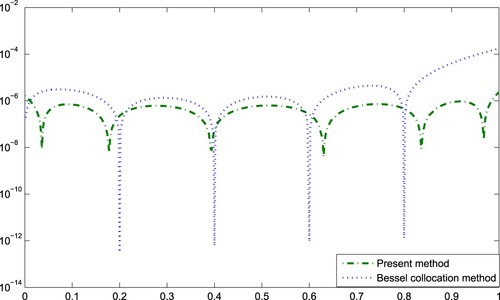Also, in Figure 2, accuracies of approximate solutions of these methods are compared.

Figure 1. Comparison of error $|e_3\left(x\right)|$.

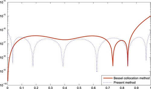
Figure 2. Accuracy of approximate solutions $|R_5\left(x\right)|$.

Example 5.2

[25]

Weconsider the Riccati differential equation with functional arguments given by $u^{\mathrm{\prime }}\left(x+2\right)-x^{2}u\left(2x-3\right)-u^2\left(x-1\right)=g\left(x\right)$ with the initial condition $u\left(0\right)=-2$.

Here, $g\left(x\right)=3+2x-19x^2+20x^3-5x^4$ and the exact solution is $u\left(x\right)=x^2-x-2$. The proposed method is applied for N = 2 and thus, we gain $u_2\left(x\right)=0.082772x^2-1.330725x-1.980444$.

Example 5.3

[20]

Now, let solve Riccati differential equation $u^{\mathrm{\prime }}\left(x\right)+u^2\left(x\right)=1$ with the initial condition $u\left(0\right)=0.$

The exact solution of problem is $u\left(x\right)=({\mathrm{e}}^{2x}-1)/({\mathrm{e}}^{2x}+1)$. Present method is applied for N = 5 and thus we compute the approximate solution

$\begin{array}{rl}{u}_5\left(x\right)& =-0.01561477x^5+0.18737947x^4-0.43144236x^3\\ & +0.02351138x^2+0.99776043x+\mathrm{0.00005064.}\end{array}$

For N = 5, M = 6 we apply the residual error method and we obtain the estimation error function

$\begin{array}{rl}{e}_{5,6}\left(x\right)& =-0.045817789219205901085629761837481x^6\\ & +0.13587872934913514111343602053239x^5\\ & -0.15233391724320338722620249427564x^4\\ & +0.079951365640905033838059523532138x^3\\ & -0.019606339297920959141574570594457x^2\\ & +0.0019152980125420472189839982135595x\\ & -\mathrm{0.000044317140260912086299066592331997.}\end{array}$

In Table 1, the numerical results are given. Namely, the absolute errors of the Taylor method [20], the Bessel collocation method [25] and the present method for N = 5, 7, 8, 9. The actual error function e₅(x) and the estimation error function e_5,6(x) are given in Figure 3.

Figure 3. Graphics of $|e_5\left(x\right)|$ and $|e_{5,6}\left(x\right)|$.

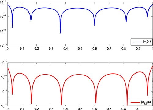
Table 1. Comparison of absolute errors.

	Taylor method [20]	Bessel collocation method [25]
x	N = 5	N = 5	N = 8
0.2	0.679776E−6	0.517341E−4	0.194715E−6
0.4	0.830377E−4	0.259692E−4	0.182778E−6
0.6	0.131843E−2	0.406570E−4	0.159478E−6
0.8	0.898722E−2	0.123901E−4	0.131850E−6
1.0	0.384058E−1	0.751414E−3	0.899933E−6
		Present method
x	N = 5	N = 7	N = 9
0.2	0.111371E−6	0.672756E−9	0.130042E−11
0.4	0.761541E−7	0.914963E−9	0.271098E−10
0.6	0.602417E−9	0.146507E−8	0.152924E−10
0.8	0.500046E−7	0.224639E−8	0.191446E−10
1.0	0.506432E−6	0.697202E−8	0.310221E−10

Example 5.4

[18]

Lastly, let solve the Riccati differential equation $u^{\mathrm{\prime }}\left(x\right)-2u+u^2\left(x\right)=1$ with the initial condition $u\left(0\right)=0.$

By applying the present method for N = 6, we obtain the approximate solution

$\begin{array}{rl}{u}_6\left(x\right)& =0.3976697967610276496230881093652x^6\\ & -0.55995447628188066424570479284739x^5\\ & -0.65736090407602398855146930145565x^4\\ & +0.56119039336426879138741696806392x^3\\ & +0.94289904938799495859313992696116x^2\\ & +1.005280244228598851563560856448x\\ & -\mathrm{0.00011285708278009885005121332168798.}\end{array}$

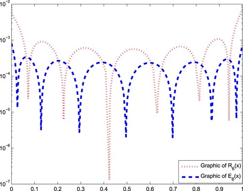
The graphic of the absolute error function for N = 7 is illustrated in Figure 4. In Figure 5, the comparison of errors is reported. In Figure 6, we give comparison of residual functions $R_N\left(x\right)$ and $E_N\left(x\right)$ for N = 6.

Figure 4. Graphic of $|e_7\left(x\right)|$.

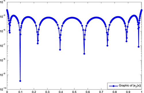
Figure 5. Absolute error functions obtained by different methods.

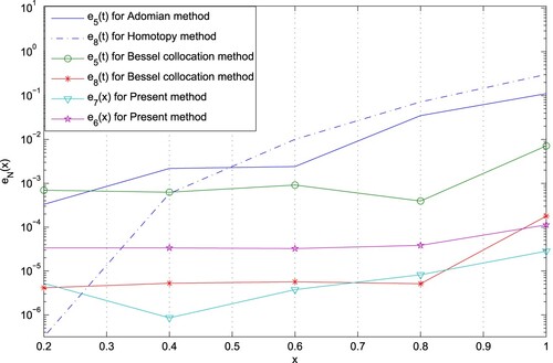
Figure 6. Comparison of the residual functions $|R_6\left(x\right)|$ and $|E_6\left(x\right)|$.

6. Conclusions

In this paper, a numerical method based on the operational matrices of integration and product for standard bases polynomials are presented to solve Riccati type differential equations with functional arguments. Indeed, the method is based on the least-squares approximation, too. There are some features of the method. For example, the method doesn't require collocation points. Moreover, the operational matrix of integration consists of zeros, so that it involves convenience in computational works. Also, the polynomials of degree N are obtained which approximate unknown function and its derivative. From numerical examples, it is can be seen errors of approximate solutions are less then errors of other methods. In addition, it is seen that the estimation errors are closed to actual errors in Examples. Therefore, it is observed that the error estimation method is efficiency. It can be used for measurement of errors when the exact solution of the problem is unknown.

Acknowledgments

The authors are supported by the Scientific Research Project Administration of Akdeniz University. Author would like to thank the reviewers for their thoughtful comments and efforts towards improving his article.

Disclosure statement

No potential conflict of interest was reported by the author(s).

Correction Statement

This article has been republished with minor changes. These changes do not impact the academic content of the article.

References

- Abbas IA. Eigenvalue approach for an unbounded medium with a spherical cavity based upon two-temperature generalized thermoelastic theory. J Mech Sci Techn. 2014;28:4193–4198. doi: 10.1007/s12206-014-0932-6
- Marini M, Ellai R, Chirila A. On solutions of Saint-Venant's problem for elastic dipolar bodies with voids. Carpathian J Math. 2017;33(2):219–232.
- Yüzbaşı Ş. Bessel collocation approach for solving one-dimensional wave equation with Dirichlet, Neumann boundary and integral conditions. Res Commun Math Mathc Sci. 2019;11(1):63–87.
- Amin R, Yüzbaşı Ş, Gao L, et al. Algorithm for the numerical solutions of volterra population growth model with fractional order via haar wavelet. Contemp Math. 2020;1(2):102–111. doi: 10.37256/cm.00056.102-111
- Celik E, Karaduman E, Bayram M. Numerical solutions of chemical differential-algebraic equations. App Math Comput. 2003;39(2–3):259–264. doi: 10.1016/S0096-3003(02)00178-9
- Merdan M. Homotopy perturbation method for solving human T-cell lymphotropic virus I (HTLV-I) infection of CD4+ T-cells model. Math Comput Appl. 2009;14(2):85–96.
- Bahaa GM, Hamiaz A. Optimal control problem for coupled time fractional diffusion systems with final observations. J Taibah Univ Sci. 2019;13(1):124–135. doi: 10.1080/16583655.2018.1545560
- Ince EL. Ordinary differential equations. London: Longmans; 1927.
- Reid WT. Riccati differential equations. New York (NY): Academic Press; 1972.
- Fraga ES. The Schrödinger and Riccati equations. Berlin (Germany): Springer; 1999. (Vol. 70 of Lecture notes in chemistry).
- Shankar R. Principles of quantum mechanics. New York (NY): Plenum; 1980.
- Lasiecka I, Triggiani R. Differential and algebraic Riccati equations with application to boundary point control problems: continuous theory and approximation theory. Berlin (Germany): Springer; 1991. (Vol. 164 of Lecture notes in control and information sciences).
- Mak MK, Harko T. New further integrability case for the Riccati equation. Appl Math Comput. 2013;219:7465–7471.
- Geng F, Lin Y, Cui M. A piecewise variational iteration method for Riccati differential equations. Comput Math Appl. 2009;58:2518–2522. doi: 10.1016/j.camwa.2009.03.063
- Ghorbani A, Momani S. An effective variational iteration algorithm for solving Riccati differential equations. Appl Math Lett. 2010;23:922–927. doi: 10.1016/j.aml.2010.04.012
- Abbasbandy S. A new application of He's variational iteration method for quadratic Riccati differential equation by using Adomian's polynomials. J Comput Appl Math. 2007;207:59–63. doi: 10.1016/j.cam.2006.07.012
- Lakestani M, Dehghan M. Numerical solution of Riccati equation using the cubic B-spline scaling functions and Chebyshev cardinal functions. Comput Phys Commun. 2010;181:957–966. doi: 10.1016/j.cpc.2010.01.008
- Abbasbandy S. Homotopy perturbation method for quadratic Riccati differential equation and comparison with Adomian's decomposition method. Appl Math Comput. 2006;172:485–490.
- Geng F. A modified variational iteration method for solving Riccati differential equations. Comput Math Appl. 2010;60:1868–1872. doi: 10.1016/j.camwa.2010.07.017
- Gulsu M, Sezer M. On the solution of the Riccati equation by the Taylor matrix method. Appl Math Comput. 2006;176:414–421.
- Abbasbandy S. Iterated He's homotopy perturbation method for quadratic Riccati differential equation. Appl Math Comput. 2006;175:581–589.
- Bulut H, Evans DJ. On the solution of the Riccati equation by the decomposition method. Int J Comput Math. 2002;79:103–109. doi: 10.1080/00207160211917
- El-Tawil MA, Bahnasawi AA, Abdel-Naby A. Solving Riccati differential equation using Adomian's decomposition method. Appl Math Comput. 2004;157:503–514.
- Aminikhah H, Hemmatnezhad M. An efficient method for quadratic Riccati differential equation. Commun Nonlinear Sci Numer Simul. 2010;15:835–839. doi: 10.1016/j.cnsns.2009.05.009
- Yüzbaşı Ş. A numerical approximation based on the Bessel functions of first kind for solutions of Riccati type differential-difference equations. Comput Math Appl. 2012;64:1691–1705. doi: 10.1016/j.camwa.2012.01.026
- Abdelgadir AA. On ground state for a class of nonlinear Schrödinger equation. J Taibah Univ Sci. 2018;12(2):138–142. doi: 10.1080/16583655.2018.1451058
- Shahoot AM, Alurrfi KAE, Elmrid MOM, et al. The (G'/G)-expansion method for solving a nonlinear PDE describing the nonlinear low-pass electrical lines. J Taibah Univ Sci. 2019;13(1):63–70. doi: 10.1080/16583655.2018.1528663
- Ghomanjani F, Khorram E. Approximate solution for quadratic Riccati differential equation. J Taibah Univ Sci. 2017;11(2):246–250. doi: 10.1016/j.jtusci.2015.04.001
- Ross SL. Differential equations. USA: Wiley; 1984.
- Corrington MS. Solution of differential and integral equations with Walsh functions. IEEE Trans Circuit Theory. 1973;CT-20(5):470–476. doi: 10.1109/TCT.1973.1083748
- Chen CF, Hsiao CH. A Walsh series direct method for solving variational problems. J Frank Inst. 1975;300:265–280. doi: 10.1016/0016-0032(75)90199-4
- Paraskevopoulos PN, Sklavounos PG, Georgiou GCh. The operational matrix of integration for Bessel functions. J Frank Inst. 1990;327:329–341. doi: 10.1016/0016-0032(90)90026-F
- Yousefi SA, Behroozifar M. Operational matrices of Bernstein polynomials and their applications. Int J of Sys Sci. 2010;41:709–716. doi: 10.1080/00207720903154783
- Chang R, Wang M. Shifted Legendre direct method for variational problem. J Optim Theory App. 1983;39:299–307. doi: 10.1007/BF00934535
- Gu J, Jiang W. The Haar wavelets operational matrix of integration. Int J Sys Sci. 1996;27:623–628. doi: 10.1080/00207729608929258
- Horng I, Chou J. Shifted Chebyshev direct method for solving variational problems. Int J Sys Sci. 1985;16:855–861. doi: 10.1080/00207728508926718
- Yüzbaşı Ş, Ismailov N. An operational matrix method for solving linear Fredholm Volterra integro-differential equations. Turkish J Math. 2018;42:243–256. doi: 10.3906/mat-1611-126
- Yüzbaşı Ş, Ismailov N. A Taylor operation method for solutions of generalized pantograph type delay differential equations. Turkish J Math. 2018;42:395–406.