Novel solitons and periodic wave solutions for Davey–Stewartson system with variable coefficients

Abstract

In this paper, the variable coefficients Davey–Stewartson system represents many physical phenomena in shallow water waves, quantum and optics, etc, is transformed directly into nonlinear ordinary differential system by using the new modification to the direct similarity reduction method. After solving the reduced system, new Jacobi, hyperbolic and periodic wave solutions are achieved for complex variable coefficients Davey–Stewartson system. The application of the new modification of the direct similarity reduction method reflects how this method is powerful, easy and simple, if it is compared with other symmetry techniques.

Keywords:

• Davey–Stewartson system with variable coefficients
• direct similarity method
• Jacobi elliptic wave functions
• hyperbolic and periodic wave solutions

1. Introduction

Recently, the aspect of solitary wave attracted many physicians as it is very common in many fields of physics, such as ocean dynamics, fluid mechanics, plasmas and optics. Moreover, when the solitary wave keeps its shape after interaction with other solitary waves, it becomes a soliton. Therefore, solitons also are important in many fields, especially quantum mechanics and optics. From a different point of view, solitary waves and solitons are considered solutions for many famous models in partial differential equations, as for example Korteweg de-Vries (KdV) and the Nonlinear Schrodinger (NLS) equations [1–8].

Therefore, many new methodologies, for example, tanh method, direct algebric method, Darboux transformation, Painlevé test, integral methods, Bä cklund transformation, trail equation method, etc [9–26], are constructed for obtaining solitary and soliton wave solutions to nonlinear partial differential equations (NPDEs), but symmetry methods are still the most important techniques in construction and exploitation of nature laws for NPDEs [27–33]. Many modifications and generalizations are made for symmetry to deal with different types of NPDEs. For instance, Fan [34] merges the classical Clarkson and Kruskal (CK) direct similarity reduction method with the homogeneous balance method to make it easier. Then, Moussa et al. [35,36] and Elshiekh [37–40] expanded it further to solve NPDEs with variable coefficients.

The importance of the direct similarity reduction CK method combined with homogeneous balance method is the direct reduction of n-dimensional NPDE to an ordinary differential equation. On the other hand, other symmetry methods reduce the n-dimensional NPDEs to (n−1)-dimensional NPDEs. Therefore, the symmetry method or other methods should be used to reduce those equations again.

In this study, the direct similarity method has been modified in order to apply it on the complex variable-coefficient systems. As one example, this method will be applied on the following variable coefficients (Davey–Stewartson (vcDS) system): (1) $\begin{array}{rl}& i{\mathrm{\Psi }}_t+a_1\left(t\right){\mathrm{\Psi }}_{xx}+a_2\left(t\right){\mathrm{\Psi }}_{yy}-b_1\left(t\right){\left|\mathrm{\Psi }\right|}^2\mathrm{\Psi }\\ & +b_2\left(t\right)\mathrm{\Psi }\mathrm{\Phi }=0,\\ & s_1{\mathrm{\Phi }}_{xx}-{\mathrm{\Phi }}_{yy}=s_2{\left|\mathrm{\Psi }\right|}_{xx}^2,\end{array}$(1) where $\mathrm{\Psi }=\mathrm{\Psi }(t,x,y)$, and $\mathrm{\Phi }=\mathrm{\Phi }(t,x,y)$ are the complex wave envelope and the real forcing terms, respectively. Note that $a_1$, $a_2$, $b_1$ and $b_2$ are real functions in t, where $a_1$and $a_2$ are corresponding to the group velocity dispersion (GVD) terms and $b_1$ and $b_2$ represent the nonlinear cubic coefficient and quadratic nonlinearity terms while $s_1$ and $s_2$ are real constants (for more details about the physical background of the vcDS system see [41,42]). Recently, Zhou et al. [41] solve the vcDs for Lax pair and Bäcklund transformation. Moreover, Wei et al. [42] obtain conservation laws and similarity solutions using the classical Lie group.

2. Methodology

In this paper, one more modification for the direct similarity reduction method will be applied [35–40] to transform complex vcNPDEs systems to nonlinear ordinary differential systems:

Consider a vcNPDEs system as follows: (2) $S_k(t,x,y,{\mathrm{\Psi }}_x,{\mathrm{\Psi }}_{xx},{\mathrm{\Psi }}_t,{\mathrm{\Phi }}_x,\dots ,a_i\left(t\right),b_j\left(t\right))=0,$(2) where $a_i(t)$ and $b_j(t)$ are arbitrary functions in t, k = 2 and i and j are some positive integers. In the following steps, system (1(1) $\begin{array}{rl}& i{\mathrm{\Psi }}_t+a_1\left(t\right){\mathrm{\Psi }}_{xx}+a_2\left(t\right){\mathrm{\Psi }}_{yy}-b_1\left(t\right){\left|\mathrm{\Psi }\right|}^2\mathrm{\Psi }\\ & +b_2\left(t\right)\mathrm{\Psi }\mathrm{\Phi }=0,\\ & s_1{\mathrm{\Phi }}_{xx}-{\mathrm{\Phi }}_{yy}=s_2{\left|\mathrm{\Psi }\right|}_{xx}^2,\end{array}$(1) ) is transformed directly to a system of nonlinear ordinary differential equations as follows:

1. Assume (3) $\begin{array}{rl}\mathrm{\Psi }(t,x,y)& =\frac{{\mathrm{\partial }}^{m_1}}{\mathrm{\partial }{x}_{m_1}}\psi \left(\varpi (t,x,y)\right){\mathrm{e}}^{(\mathrm{i}(\varrho \left(t\right)+c_{1}x+c_{2}y))},\\ \mathrm{\Phi }(t,x,y)& =\frac{{\mathrm{\partial }}^{m_2}}{\mathrm{\partial }{x}_{m_2}}\varphi \left(\varpi (t,x,y)\right),\end{array}$(3) where ϖ is the newly independent variable and ψ and φ are the new dependent similarity variables, respectively, $c_1$ and $c_2$ are undetermined constants. Moreover, $\varrho (t)$ is an unknown function on t and $m_1$ and $m_2$ represent positive integers obtained from balancing between nonlinear and linear terms in system (1(1) $\begin{array}{rl}& i{\mathrm{\Psi }}_t+a_1\left(t\right){\mathrm{\Psi }}_{xx}+a_2\left(t\right){\mathrm{\Psi }}_{yy}-b_1\left(t\right){\left|\mathrm{\Psi }\right|}^2\mathrm{\Psi }\\ & +b_2\left(t\right)\mathrm{\Psi }\mathrm{\Phi }=0,\\ & s_1{\mathrm{\Phi }}_{xx}-{\mathrm{\Phi }}_{yy}=s_2{\left|\mathrm{\Psi }\right|}_{xx}^2,\end{array}$(1) ).

2. Collect the coefficients of $\psi ,\varphi$ and its derivatives.

3. Assume that the normalized coefficient is the greatest linear term, then collect the same derivatives and powers of ψ and φ and equate them with any arbitrary functions ${\mathrm{\Omega }}_l(\varpi )$ multiplied with the normalized coefficient. After that, a partial differential system in $\varpi (t,x,y)$ is obtained where l is a positive integer.

4. If $\varpi (t,x,y)$ takes the form $\mathrm{\Omega }(\varpi )={\varpi }_0(t,x,y),$ then assume that $\mathrm{\Omega }(\varpi )=\varpi$.

3. Similarity reductions and solutions

In this section, the vcDS system (1(1) $\begin{array}{rl}& i{\mathrm{\Psi }}_t+a_1\left(t\right){\mathrm{\Psi }}_{xx}+a_2\left(t\right){\mathrm{\Psi }}_{yy}-b_1\left(t\right){\left|\mathrm{\Psi }\right|}^2\mathrm{\Psi }\\ & +b_2\left(t\right)\mathrm{\Psi }\mathrm{\Phi }=0,\\ & s_1{\mathrm{\Phi }}_{xx}-{\mathrm{\Phi }}_{yy}=s_2{\left|\mathrm{\Psi }\right|}_{xx}^2,\end{array}$(1) ) is going to be transformed to only one-dimensional nonlinear differential system using direct similarity method as follows:

Using the balancing technique between the nonlinear terms $|\mathrm{\Psi }{|}^2\mathrm{\Psi }$ and $\mathrm{\Psi }\mathrm{\Phi }$ and the dispersive term ${\mathrm{\Psi }}_{xx}$ in the first equation of the system (1(1) $\begin{array}{rl}& i{\mathrm{\Psi }}_t+a_1\left(t\right){\mathrm{\Psi }}_{xx}+a_2\left(t\right){\mathrm{\Psi }}_{yy}-b_1\left(t\right){\left|\mathrm{\Psi }\right|}^2\mathrm{\Psi }\\ & +b_2\left(t\right)\mathrm{\Psi }\mathrm{\Phi }=0,\\ & s_1{\mathrm{\Phi }}_{xx}-{\mathrm{\Phi }}_{yy}=s_2{\left|\mathrm{\Psi }\right|}_{xx}^2,\end{array}$(1) ), we get $m_1=1$ and $m_2=2$. Therefore, Equation (3(3) $\begin{array}{rl}\mathrm{\Psi }(t,x,y)& =\frac{{\mathrm{\partial }}^{m_1}}{\mathrm{\partial }{x}_{m_1}}\psi \left(\varpi (t,x,y)\right){\mathrm{e}}^{(\mathrm{i}(\varrho \left(t\right)+c_{1}x+c_{2}y))},\\ \mathrm{\Phi }(t,x,y)& =\frac{{\mathrm{\partial }}^{m_2}}{\mathrm{\partial }{x}_{m_2}}\varphi \left(\varpi (t,x,y)\right),\end{array}$(3) ) becomes (4) $\begin{array}{rl}\mathrm{\Psi }& =\frac{\mathrm{\partial }}{\mathrm{\partial }x}\psi \left(\varpi (t,x,y)\right){\mathrm{e}}^{(\mathrm{i}(\varrho \left(t\right)+c_{1}x+c_{2}y))}\\ & ={\varpi }_x{\psi }^{\mathrm{\prime }}\left(\varpi (t,x,y)\right){\mathrm{e}}^{(\mathrm{i}(\varrho \left(t\right)+c_{1}x+c_{2}y))},\\ \mathrm{\Phi }& =\frac{{\mathrm{\partial }}^2}{\mathrm{\partial }{t}^2}\varphi \left(\varpi (t,x,y)\right)\\ & ={\varphi }^{\mathrm{\prime }\mathrm{\prime }}\left(\varpi (x,y,t)\right)w_x^2+{\varphi }^{\mathrm{\prime }}\left(\varpi (t,x,y)\right){\varpi }_{xx}.\end{array}$(4) Substituting in system (1(1) $\begin{array}{rl}& i{\mathrm{\Psi }}_t+a_1\left(t\right){\mathrm{\Psi }}_{xx}+a_2\left(t\right){\mathrm{\Psi }}_{yy}-b_1\left(t\right){\left|\mathrm{\Psi }\right|}^2\mathrm{\Psi }\\ & +b_2\left(t\right)\mathrm{\Psi }\mathrm{\Phi }=0,\\ & s_1{\mathrm{\Phi }}_{xx}-{\mathrm{\Phi }}_{yy}=s_2{\left|\mathrm{\Psi }\right|}_{xx}^2,\end{array}$(1) ) and collecting the different powers and derivatives, we achieved the following system (5) $\begin{array}{rl}& (a_1\left(t\right){\varpi }_x^3+a_2\left(t\right){\varpi }_y^2{\varpi }_x){\psi }^{\mathrm{\prime }\mathrm{\prime }\mathrm{\prime }}+b_2\left(t\right){\varpi }_x^3{\varphi }^{\mathrm{\prime }\mathrm{\prime }}{\psi }^{\mathrm{\prime }}\\ & +b_2\left(t\right){\varpi }_x{\varpi }_{xx}{\varphi }^{\mathrm{\prime }}{\psi }^{\mathrm{\prime }}-b_1\left(t\right){\varpi }_x^3{\psi }^{\mathrm{\prime }3}\\ & +[I({\varpi }_t+2a_2\left(t\right)c_2{\varpi }_y+2a_1\left(t\right)c_1{\varpi }_x){\varpi }_x\\ & +a_2\left(t\right)w_x{w}_{yy}+3a_1\left(t\right){\varpi }_x{\varpi }_{xx}\\ & +2a_2\left(t\right){\varpi }_{xy}{\varpi }_y]{\psi }^{\mathrm{\prime }\mathrm{\prime }}\\ & +[I{({\varpi }_t+2a_2\left(t\right)c_2{\varpi }_y+2a_1\left(t\right)c_1{\varpi }_x)}_x\\ & -a_1\left(t\right)c_1^2{\varpi }_x\\ & +a_1\left(t\right){\varpi }_{xxx}-a_2\left(t\right)c_2^2{\varpi }_x\\ & -{\varrho }^{\mathrm{\prime }}\left(t\right){\varpi }_x+a_2\left(t\right){\varpi }_{xyy}]{\psi }^{\mathrm{\prime }}=0,\end{array}$(5) (6) $\begin{array}{rl}& (s_1{\varpi }_x^4-{\varpi }_x^2{\varpi }_y^2){\varphi }^{\mathrm{\prime }\mathrm{\prime }\mathrm{\prime }\mathrm{\prime }}+(6s_1{\varpi }_x^2{\varpi }_{xx}-4{\varpi }_x{\varpi }_y{\varpi }_{xy}\\ & -{\varpi }_x^2{\varpi }_{yy}-{\varpi }_{xx}{\varpi }_y^2){\varphi }^{\mathrm{\prime }\mathrm{\prime }\mathrm{\prime }}\\ & [s_1(3{\varpi }_{xx}^2+4{\varpi }_x{\varpi }_{xxx})-2{\varpi }_{xy}^2-2{\varpi }_x{\varpi }_{xyy}\\ & -{\varpi }_{yy}{\varpi }_{xx}-2{\varpi }_y{\varpi }_{xxy}]{\varphi }^{\mathrm{\prime }\mathrm{\prime }}\\ & +(s_1{\varpi }_{xxxx}-{\varpi }_{xxyy}){\varphi }^{\mathrm{\prime }}-2s_2{\varpi }_x^4{\psi }^{\mathrm{\prime }\mathrm{\prime }2}\\ & -10s_2{\varpi }_x^2{\varpi }_{xx}{\psi }^{\mathrm{\prime }}{\psi }^{\mathrm{\prime }\mathrm{\prime }}\\ & -2s_2({\varpi }_x^4{\psi }^{\mathrm{\prime }}{\psi }^{\mathrm{\prime }\mathrm{\prime }\mathrm{\prime }}+{\varpi }_{xx}^2{\psi }^{\mathrm{\prime }2}+{\varpi }_x{\varpi }_{xxx}{\psi }^{\mathrm{\prime }2})=0.\end{array}$(6) Taking $(a_1(t){\varpi }_x^3+a_2(t){\varpi }_y^2{\varpi }_x)$ as a normalized coefficient and equating the different powers and derivatives of φ and ψ by $(a_1(t){\varpi }_x^3+a_2(t){\varpi }_y^2{\varpi }_x){\mathrm{\Gamma }}_l(\varpi )$. Therefore, the result will be a system of partial differential equations in ϖ. By solving it using step $(4)$, system (1(1) $\begin{array}{rl}& i{\mathrm{\Psi }}_t+a_1\left(t\right){\mathrm{\Psi }}_{xx}+a_2\left(t\right){\mathrm{\Psi }}_{yy}-b_1\left(t\right){\left|\mathrm{\Psi }\right|}^2\mathrm{\Psi }\\ & +b_2\left(t\right)\mathrm{\Psi }\mathrm{\Phi }=0,\\ & s_1{\mathrm{\Phi }}_{xx}-{\mathrm{\Phi }}_{yy}=s_2{\left|\mathrm{\Psi }\right|}_{xx}^2,\end{array}$(1) ) is reduced to the following nonlinear ordinary system (7) $\begin{array}{rl}& k_1{\psi }^{\mathrm{\prime }3}+{\lambda }_0{\psi }^{\mathrm{\prime }}-k_2{\psi }^{\mathrm{\prime }}{\varphi }^{\mathrm{\prime }\mathrm{\prime }}-{\psi }^{\mathrm{\prime }\mathrm{\prime }\mathrm{\prime }}=0,\end{array}$(7) (8) $\begin{array}{rl}& (s_1{m}_1^2-m_2^2){\varphi }^{\mathrm{\prime }\mathrm{\prime }\mathrm{\prime }\mathrm{\prime }}=m_1^2{s}_2({\psi }^{\mathrm{\prime }2}{)}^{\mathrm{\prime }\mathrm{\prime }},\end{array}$(8) where ${\lambda }_0,m_1,m_2,$ $k_1$ and $k_2$ are arbitrary constants. With similarity variables (9) $\begin{array}{rl}\mathrm{\Psi }& =m_1{\psi }^{\mathrm{\prime }}\left(\varpi (t,x,y)\right)\\ & {\mathrm{e}}^{(\mathrm{i}(c_{1}x+c_{2}y-\int ((c_1^2-{\lambda }_0{m}_1^2)a_1\left(t\right)+(c_2^2-\lambda 0m_2^2)a_2\left(t\right))\mathrm{d}t))},\\ \mathrm{\Phi }& ={\varphi }^{\mathrm{\prime }\mathrm{\prime }}\left(\varpi (t,x,y)\right)m_1^2,\mathrm{where}\\ \varpi & =m_{1}x+m_{2}y-2\int (c_1{m}_1{a}_1\left(t\right)+c_2{m}_2{a}_2\left(t\right))\mathrm{d}t,\end{array}$(9)

and the following conditions between the variable coefficients (10) $\begin{array}{rl}{b}_1\left(t\right)& =\frac{k_1}{m_1^2}(m_1^2{a}_1\left(t\right)+m_2^2{a}_2\left(t\right)),\\ b_2\left(t\right)& =\frac{k_2}{m_1^2}(m_1^2{a}_1\left(t\right)+m_2^2{a}_2\left(t\right)).\end{array}$(10) Integrate Equation (8(8) $\begin{array}{rl}& (s_1{m}_1^2-m_2^2){\varphi }^{\mathrm{\prime }\mathrm{\prime }\mathrm{\prime }\mathrm{\prime }}=m_1^2{s}_2({\psi }^{\mathrm{\prime }2}{)}^{\mathrm{\prime }\mathrm{\prime }},\end{array}$(8) ) twice (11) ${\varphi }^{\mathrm{\prime }\mathrm{\prime }}=\frac{s_2{m}_1^2}{(s_1{m}_1^2-m_2^2)}{\psi }^{\mathrm{\prime }2}+A_1\varpi +A_2,$(11) where $A_1$ and $A_2$ are integration constants. By substituting from Equation (11(11) ${\varphi }^{\mathrm{\prime }\mathrm{\prime }}=\frac{s_2{m}_1^2}{(s_1{m}_1^2-m_2^2)}{\psi }^{\mathrm{\prime }2}+A_1\varpi +A_2,$(11) ) into Equation (7(7) $\begin{array}{rl}& k_1{\psi }^{\mathrm{\prime }3}+{\lambda }_0{\psi }^{\mathrm{\prime }}-k_2{\psi }^{\mathrm{\prime }}{\varphi }^{\mathrm{\prime }\mathrm{\prime }}-{\psi }^{\mathrm{\prime }\mathrm{\prime }\mathrm{\prime }}=0,\end{array}$(7) ) and by integration with respect to w assuming that $A_1=0$, Equation (7(7) $\begin{array}{rl}& k_1{\psi }^{\mathrm{\prime }3}+{\lambda }_0{\psi }^{\mathrm{\prime }}-k_2{\psi }^{\mathrm{\prime }}{\varphi }^{\mathrm{\prime }\mathrm{\prime }}-{\psi }^{\mathrm{\prime }\mathrm{\prime }\mathrm{\prime }}=0,\end{array}$(7) ) becomes (12) $\begin{array}{rl}& \frac{1}{2}(k_1-\frac{k_2{s}_2{m}_1^2}{(s_1{m}_1^2-m_2^2)}){\psi }^{\mathrm{\prime }4}\\ & +({\lambda }_0-k_2{A}_2){\psi }^{\mathrm{\prime }2}-{\psi }^{\mathrm{\prime }\mathrm{\prime }2}=k_0,\end{array}$(12) where $k_0$ is an integration constant. Use ${\psi }^{\mathrm{\prime }}=\vartheta ,$ the following Riccati equation is obtained (13) $\begin{array}{rl}{\vartheta }^{\mathrm{\prime }2}& =\frac{1}{2}(k_1-\frac{k_2{s}_2{m}_1^2}{(s_1{m}_1^2-m_2^2)}){\vartheta }^4\\ & +({\lambda }_0-k_2{A}_2){\vartheta }^2+k_0.\end{array}$(13) Equation (13(13) $\begin{array}{rl}{\vartheta }^{\mathrm{\prime }2}& =\frac{1}{2}(k_1-\frac{k_2{s}_2{m}_1^2}{(s_1{m}_1^2-m_2^2)}){\vartheta }^4\\ & +({\lambda }_0-k_2{A}_2){\vartheta }^2+k_0.\end{array}$(13) ) has the following Jacobi elliptic-type solutions (14) $\begin{array}{rl}& {\vartheta }_1=SN(\varpi ,\pm \sqrt{\frac{1}{2}(k_1-\frac{k_2{s}_2{m}_1^2}{(s_1{m}_1^2-m_2^2)})}),\\ {\vartheta }_2& =CD(\varpi ,\pm \sqrt{\frac{1}{2}(k_1-\frac{k_2{s}_2{m}_1^2}{(s_1{m}_1^2-m_2^2)})}),\\ & \mathrm{with}{\lambda }_0=k_2{A}_2-\frac{1}{2}(k_1-\frac{k_2{s}_2{m}_1^2}{(s_1{m}_1^2-m_2^2)})-1.\end{array}$(14) (15) $\begin{array}{rl}& {\vartheta }_3=CN(\varpi ,\pm \sqrt{\frac{1}{2}(\frac{k_2{s}_2{m}_1^2}{(s_1{m}_1^2-m_2^2)}-k_1)}),\mathrm{where}\\ {\lambda }_0& =k_2{A}_2+\frac{k_2{s}_2{m}_1^2}{(s_1{m}_1^2-m_2^2)}-k_1-1.\end{array}$(15) (16) $\begin{array}{rl}& {\vartheta }_4=DN(\varpi ,\pm \sqrt{2-{\lambda }_0+k_2{A}_2}),\mathrm{with}\\ & k_1=\frac{k_2{s}_2{m}_1^2}{(s_1{m}_1^2-m_2^2)}-2.\end{array}$(16) (17) $\begin{array}{rl}& {\vartheta }_5=NS(\varpi ,\pm \sqrt{k_2{A}_2-{\lambda }_0-1}),\mathrm{where}\\ & k_1=\frac{k_2{s}_2{m}_1^2}{(s_1{m}_1^2-m_2^2)}+2.\end{array}$(17) (18) $\begin{array}{rl}& {\vartheta }_6=DC(\varpi ,\pm \sqrt{k_2{A}_2-{\lambda }_0-1}),\mathrm{where}\\ & k_1=\frac{k_2{s}_2{m}_1^2}{(s_1{m}_1^2-m_2^2)}+2.\end{array}$(18) (19) $\begin{array}{rl}& {\vartheta }_7=NC(\varpi ,\pm \sqrt{1+\frac{1}{2}(\frac{k_2{s}_2{m}_1^2}{(s_1{m}_1^2-m_2^2)}-k_1)}),\\ & \mathrm{with}{\lambda }_0=1+k_2{A}_2-k_1+\frac{k_2{s}_2{m}_1^2}{(s_1{m}_1^2-m_2^2)}.\end{array}$(19) (20) $\begin{array}{rl}& {\vartheta }_8=ND(\varpi ,\pm \sqrt{1-\frac{1}{2}(\frac{k_2{s}_2{m}_1^2}{(s_1{m}_1^2-m_2^2)}-k_1)}),\\ & \mathrm{with}{\lambda }_0=1+k_2{A}_2-\frac{1}{2}(k_1-\frac{k_2{s}_2{m}_1^2}{(s_1{m}_1^2-m_2^2)}).\end{array}$(20) (21) $\begin{array}{rl}& {\vartheta }_9=SC(\varpi ,\pm \sqrt{1-\frac{1}{2}(\frac{k_2{s}_2{m}_1^2}{(s_1{m}_1^2-m_2^2)}-k_1)}),\\ & \mathrm{where}{\lambda }_0=1+k_2{A}_2+\frac{1}{2}(k_1-\frac{k_2{s}_2{m}_1^2}{(s_1{m}_1^2-m_2^2)}).\end{array}$(21) (22) $\begin{array}{rl}& {\vartheta }_{10}=SD(\varpi ,\pm \sqrt{\frac{1}{2}M}),\mathrm{with}M=(1+{\lambda }_0-k_2{A}_2),\\ & k_1=\frac{k_2{s}_2{m}_1^2}{(s_1{m}_1^2-m_2^2)}-M(1-\frac{1}{2}M).\end{array}$(22) (23) $\begin{array}{rl}& {\vartheta }_{11}=CS(\varpi ,\pm \sqrt{2-{\lambda }_0+k_2{A}_2}),\\ & \mathrm{where}{k}_1=\frac{k_2{s}_2{m}_1^2}{(s_1{m}_1^2-m_2^2)}+2.\end{array}$(23) (24) $\begin{array}{rl}& {\vartheta }_{12}=DS(\varpi ,\pm \sqrt{\frac{1}{2}(1+{\lambda }_0-k_2{A}_2)}),\mathrm{with}\\ & k_1=\frac{k_2{s}_2{m}_1^2}{(s_1{m}_1^2-m_2^2)}+2.\end{array}$(24) (25) $\begin{array}{rl}& {\vartheta }_{13}=NS(\varpi ,\pm \sqrt{\frac{1}{2}(1-2({\lambda }_0-k_2{A}_2))})\\ & \pm CS(\varpi ,\pm \sqrt{\frac{1}{2}(1-2({\lambda }_0-k_2{A}_2))}),\mathrm{with}\\ & k_1=\frac{k_2{s}_2{m}_1^2}{(s_1{m}_1^2-m_2^2)}+\frac{1}{2}.\end{array}$(25) (26) $\begin{array}{rl}& {\vartheta }_{14}=NC(w,\pm \sqrt{1+2(\frac{k_2{s}_2{m}_1^2}{(s_1{m}_1^2-m_2^2)}-k_1)})\\ & \pm SC(w,\pm \sqrt{1+2(\frac{k_2{s}_2{m}_1^2}{(s_1{m}_1^2-m_2^2)}-k_1)})\mathrm{with}\\ & {\lambda }_0=1+k_2{A}_2-k_1+\frac{k_2{s}_2{m}_1^2}{(s_1{m}_1^2-m_2^2)}.\end{array}$(26) (27) $\begin{array}{rl}& {\vartheta }_{15}=NS(\varpi ,\pm \sqrt{2({\lambda }_0-k_2{A}_2)+2})\\ & \pm DS(\varpi ,\pm \sqrt{2({\lambda }_0-k_2{A}_2)+2}),\\ & \mathrm{with}{k}_1=\frac{k_2{s}_2{m}_1^2}{(s_1{m}_1^2-m_2^2)}+\frac{1}{2}.\end{array}$(27) If the module of Jacobi elliptic functions approach 1, it transforms to hypergeometric functions: (28) $\begin{array}{rl}{\vartheta }_{1\to 1}& =\tanh (\varpi ),{\lambda }_0=k_2{A}_2-2,\\ k_1& =2+\frac{k_2{s}_2{m}_1^2}{(s_1{m}_1^2-m_2^2)}.\end{array}$(28) (29) $\begin{array}{rl}{\vartheta }_{3\to 1}& =\mathrm{sech}(\varpi ),{\lambda }_0=k_2{A}_2-2,\\ k_1& =\frac{k_2{s}_2{m}_1^2}{(s_1{m}_1^2-m_2^2)}-2.\end{array}$(29) (30) $\begin{array}{rl}{\vartheta }_{5\to 1}& =\coth (\varpi ),{\lambda }_0=k_2{A}_2-2,\\ k_1& =2+\frac{k_2{s}_2{m}_1^2}{(s_1{m}_1^2-m_2^2)}.\end{array}$(30) (31) $\begin{array}{rl}{\vartheta }_{7\to 1}& =\cosh (\varpi ),{\lambda }_0=k_2{A}_2+1,\\ k_1& =\frac{k_2{s}_2{m}_1^2}{(s_1{m}_1^2-m_2^2)}.\end{array}$(31) (32) $\begin{array}{rl}{\vartheta }_{9\to 1}& =\sinh (\varpi ),{\lambda }_0=k_2{A}_2+1,\\ k_1& =\frac{k_2{s}_2{m}_1^2}{(s_1{m}_1^2-m_2^2)}.\end{array}$(32) (33) $\begin{array}{rl}{\vartheta }_{11\to 1}& =\mathrm{csch}(\varpi ),{\lambda }_0=k_2{A}_2+1,\\ k_1& =2+\frac{k_2{s}_2{m}_1^2}{(s_1{m}_1^2-m_2^2)}.\end{array}$(33) (34) $\begin{array}{rl}{\vartheta }_{13\to 1}& =(\coth (\varpi )\pm \mathrm{csch}(\varpi )),{\lambda }_0=k_2{A}_2-\frac{1}{2},\\ k_1& =\frac{1}{2}+\frac{k_2{s}_2{m}_1^2}{(s_1{m}_1^2-m_2^2)}.\end{array}$(34) (35) $\begin{array}{rl}{\vartheta }_{14\to 1}& =(\cosh (\varpi )\pm \sinh (\varpi )),{\lambda }_0=k_2{A}_2+1,\\ k_1& =\frac{k_2{s}_2{m}_1^2}{(s_1{m}_1^2-m_2^2)}.\end{array}$(35) Also, if the module of Jacobi elliptic functions approach zero, it becomes as periodic wave functions: (36) $\begin{array}{rl}{\vartheta }_{1\to 0}& =\sin (\varpi ),{\lambda }_0=k_2{A}_2-1,\\ k_1& =\frac{k_2{s}_2{m}_1^2}{(s_1{m}_1^2-m_2^2)}.\end{array}$(36) (37) $\begin{array}{rl}{\vartheta }_{3\to 0}& =\cos (\varpi ),{\lambda }_0=k_2{A}_2-1,\\ k_1& =\frac{k_2{s}_2{m}_1^2}{(s_1{m}_1^2-m_2^2)}.\end{array}$(37) (38) $\begin{array}{rl}{\vartheta }_{5\to 0}& =\csc (\varpi ),{\lambda }_0=k_2{A}_2-1,\\ k_1& =2+\frac{k_2{s}_2{m}_1^2}{(s_1{m}_1^2-m_2^2)}.\end{array}$(38) (39) $\begin{array}{rl}{\vartheta }_{7\to 0}& =\sec (\varpi ),{\lambda }_0=k_2{A}_2-1,\\ k_1& =2+\frac{k_2{s}_2{m}_1^2}{(s_1{m}_1^2-m_2^2)}.\end{array}$(39) (40) $\begin{array}{rl}{\vartheta }_{9\to 0}& =\tan (\varpi ),{\lambda }_0=k_2{A}_2+2,\\ k_1& =2+\frac{k_2{s}_2{m}_1^2}{(s_1{m}_1^2-m_2^2)}.\end{array}$(40) (41) $\begin{array}{rl}{\vartheta }_{11\to 0}& =\cot (\varpi ),{\lambda }_0=k_2{A}_2+2,\\ k_1& =2+\frac{k_2{s}_2{m}_1^2}{(s_1{m}_1^2-m_2^2)}.\end{array}$(41) (42) $\begin{array}{rl}{\vartheta }_{13\to 0}& =(\csc (\varpi )\pm \cot (\varpi )),{\lambda }_0=k_2{A}_2+\frac{1}{2},\\ k_1& =\frac{1}{2}+\frac{k_2{s}_2{m}_1^2}{(s_1{m}_1^2-m_2^2)}.\end{array}$(42) (43) $\begin{array}{rl}{\vartheta }_{14\to 0}& =(\sec (\varpi )\pm \tan (\varpi )),{\lambda }_0=k_2{A}_2+\frac{1}{2},\\ k_1& =\frac{1}{2}+\frac{k_2{s}_2{m}_1^2}{(s_1{m}_1^2-m_2^2)}.\end{array}$(43) (44) $\begin{array}{rl}{\vartheta }_{15\to 0}& =2\csc (\varpi ),{\lambda }_0=k_2{A}_2-1,\\ k_1& =\frac{1}{2}+\frac{k_2{s}_2{m}_1^2}{(s_1{m}_1^2-m_2^2)}.\end{array}$(44) Substituting from Equations (14(14) $\begin{array}{rl}& {\vartheta }_1=SN(\varpi ,\pm \sqrt{\frac{1}{2}(k_1-\frac{k_2{s}_2{m}_1^2}{(s_1{m}_1^2-m_2^2)})}),\\ {\vartheta }_2& =CD(\varpi ,\pm \sqrt{\frac{1}{2}(k_1-\frac{k_2{s}_2{m}_1^2}{(s_1{m}_1^2-m_2^2)})}),\\ & \mathrm{with}{\lambda }_0=k_2{A}_2-\frac{1}{2}(k_1-\frac{k_2{s}_2{m}_1^2}{(s_1{m}_1^2-m_2^2)})-1.\end{array}$(14) )–(44(44) $\begin{array}{rl}{\vartheta }_{15\to 0}& =2\csc (\varpi ),{\lambda }_0=k_2{A}_2-1,\\ k_1& =\frac{1}{2}+\frac{k_2{s}_2{m}_1^2}{(s_1{m}_1^2-m_2^2)}.\end{array}$(44) ) in (9(9) $\begin{array}{rl}\mathrm{\Psi }& =m_1{\psi }^{\mathrm{\prime }}\left(\varpi (t,x,y)\right)\\ & {\mathrm{e}}^{(\mathrm{i}(c_{1}x+c_{2}y-\int ((c_1^2-{\lambda }_0{m}_1^2)a_1\left(t\right)+(c_2^2-\lambda 0m_2^2)a_2\left(t\right))\mathrm{d}t))},\\ \mathrm{\Phi }& ={\varphi }^{\mathrm{\prime }\mathrm{\prime }}\left(\varpi (t,x,y)\right)m_1^2,\mathrm{where}\\ \varpi & =m_{1}x+m_{2}y-2\int (c_1{m}_1{a}_1\left(t\right)+c_2{m}_2{a}_2\left(t\right))\mathrm{d}t,\end{array}$(9) ), the following new generalized solitary wave solutions are obtained for the vcDS system (45) $\begin{array}{rl}& {\mathrm{\Psi }}_m(t,x,y)=m_1{\vartheta }_m(\varpi (t,x,y))\\ & {\mathrm{e}}^{(\mathrm{i}(c_{1}x+c_{2}y-2\int ((c_1^2-{\lambda }_0{m}_1^2)a_1\left(t\right)+(c_2^2-{\lambda }_0{m}_2^2)a_2\left(t\right))\mathrm{d}t))},\\ & m=1,\dots ,15.\\ & {\mathrm{\Phi }}_m(t,x,y)=(\frac{s_2{m}_1^4}{(s_1{m}_1^2-m_2^2)}{\vartheta }_m^2(\varpi (t,x,y))+A_2),\\ & \mathrm{with}\\ & \varpi (t,x,y)=m_{1}x+m_{2}y\\ & -2\int (c_1{m}_1{a}_1\left(t\right)+c_2{m}_2{a}_2\left(t\right))\mathrm{d}t,\end{array}$(45) where $m=1,2,3,\dots ,15$, ${\vartheta }_m$ are given by Equations (14(14) $\begin{array}{rl}& {\vartheta }_1=SN(\varpi ,\pm \sqrt{\frac{1}{2}(k_1-\frac{k_2{s}_2{m}_1^2}{(s_1{m}_1^2-m_2^2)})}),\\ {\vartheta }_2& =CD(\varpi ,\pm \sqrt{\frac{1}{2}(k_1-\frac{k_2{s}_2{m}_1^2}{(s_1{m}_1^2-m_2^2)})}),\\ & \mathrm{with}{\lambda }_0=k_2{A}_2-\frac{1}{2}(k_1-\frac{k_2{s}_2{m}_1^2}{(s_1{m}_1^2-m_2^2)})-1.\end{array}$(14) )–(44(44) $\begin{array}{rl}{\vartheta }_{15\to 0}& =2\csc (\varpi ),{\lambda }_0=k_2{A}_2-1,\\ k_1& =\frac{1}{2}+\frac{k_2{s}_2{m}_1^2}{(s_1{m}_1^2-m_2^2)}.\end{array}$(44) ).

4. Results and discussion

Many novel wave solutions have been obtained in the previous section are considered new for the vcDS compared to other solutions obtained previously in the literature [22,41,42]. In this section, a discussion for the plots of the complex wave envelope $|{\mathrm{\Psi }}_1|$, by assuming that $m_2=0$ in (8(8) $\begin{array}{rl}& (s_1{m}_1^2-m_2^2){\varphi }^{\mathrm{\prime }\mathrm{\prime }\mathrm{\prime }\mathrm{\prime }}=m_1^2{s}_2({\psi }^{\mathrm{\prime }2}{)}^{\mathrm{\prime }\mathrm{\prime }},\end{array}$(8) ), are presented. In this case, from Equation (9(9) $\begin{array}{rl}\mathrm{\Psi }& =m_1{\psi }^{\mathrm{\prime }}\left(\varpi (t,x,y)\right)\\ & {\mathrm{e}}^{(\mathrm{i}(c_{1}x+c_{2}y-\int ((c_1^2-{\lambda }_0{m}_1^2)a_1\left(t\right)+(c_2^2-\lambda 0m_2^2)a_2\left(t\right))\mathrm{d}t))},\\ \mathrm{\Phi }& ={\varphi }^{\mathrm{\prime }\mathrm{\prime }}\left(\varpi (t,x,y)\right)m_1^2,\mathrm{where}\\ \varpi & =m_{1}x+m_{2}y-2\int (c_1{m}_1{a}_1\left(t\right)+c_2{m}_2{a}_2\left(t\right))\mathrm{d}t,\end{array}$(9) ) the similarity variable becomes as $\varpi =m_{1}x-2\int (c_1{m}_1{a}_1(t))\mathrm{d}t$ and it depends on the variable function $a_1(t)$ only. Subsequently, we have plotted the modulus of the periodic wave packet $|{\mathrm{\Psi }}_1|$ and its Kink soliton limit $|{\mathrm{\Psi }}_{1\to 1}|$ and the soliton solution $|{\mathrm{\Psi }}_{3\to 1}|$ according to different values of the variable coefficient $a_1(t)$ as $1,t,\sin (t)$ respectively.

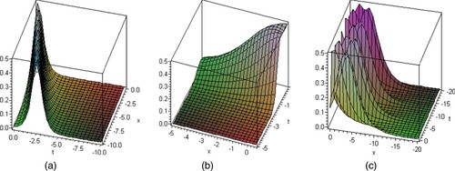
From Figures 1–3, we concluded that the propagation of the periodic, Kink soliton and soliton solutions affected by the values of the variable coefficient function $a_1(t)$.

Figure 1. Represents the periodic wave solution $|{\mathrm{\Psi }}_1|$ given by Equation (14(14) $\begin{array}{rl}& {\vartheta }_1=SN(\varpi ,\pm \sqrt{\frac{1}{2}(k_1-\frac{k_2{s}_2{m}_1^2}{(s_1{m}_1^2-m_2^2)})}),\\ {\vartheta }_2& =CD(\varpi ,\pm \sqrt{\frac{1}{2}(k_1-\frac{k_2{s}_2{m}_1^2}{(s_1{m}_1^2-m_2^2)})}),\\ & \mathrm{with}{\lambda }_0=k_2{A}_2-\frac{1}{2}(k_1-\frac{k_2{s}_2{m}_1^2}{(s_1{m}_1^2-m_2^2)})-1.\end{array}$(14) ) according to the different values of $a_1(t)$ as $1,t^2,\sin (t)$ with fixed parameters $k_1=k_2=m_1=\frac{1}{2},s_1=1,s_2=\frac{1}{4},m_2=0$ and $c_1=2$.

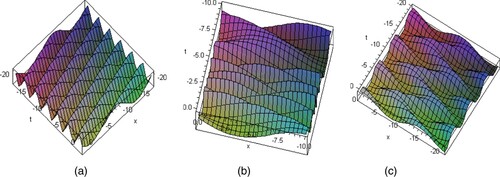
Figure 2. Shows the Kink soliton solution $|{\mathrm{\Psi }}_{1\to 1}|$ given by Equation (28(28) $\begin{array}{rl}{\vartheta }_{1\to 1}& =\tanh (\varpi ),{\lambda }_0=k_2{A}_2-2,\\ k_1& =2+\frac{k_2{s}_2{m}_1^2}{(s_1{m}_1^2-m_2^2)}.\end{array}$(28) ) according to the different values of $a_1(t)$ as $1,t,\sin (t)$ with fixed parameters $k_1=3,k_2=s_1=s_2=1,m_1=\frac{1}{2},m_2=0$ and $c_1=2$.

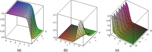
Figure 3. Represents the soliton solution $|{\mathrm{\Psi }}_{3\to 1}|$ given by Equation (29(29) $\begin{array}{rl}{\vartheta }_{3\to 1}& =\mathrm{sech}(\varpi ),{\lambda }_0=k_2{A}_2-2,\\ k_1& =\frac{k_2{s}_2{m}_1^2}{(s_1{m}_1^2-m_2^2)}-2.\end{array}$(29) ) according to the different values of $a_1(t)$ as $1,t,\sin (t)$ with fixed parameters $k_1=3,k_2=s_1=s_2=1,m_1=\frac{1}{2},m_2=0$ and $c_1=2$.

Finally, we hope that the investigation of multiply solitary and periodic wave solutions for the variable coefficients Davey–Stewartson system may shed light on new types of solitary waves generated this system in fields of hydrodynamics, plasma physics and Bose–Einstein condensates.

5. Conclusion

In this paper, the vcDS system is transformed directly into a third-order nonlinear ordinary differential system (6(6) $\begin{array}{rl}& (s_1{\varpi }_x^4-{\varpi }_x^2{\varpi }_y^2){\varphi }^{\mathrm{\prime }\mathrm{\prime }\mathrm{\prime }\mathrm{\prime }}+(6s_1{\varpi }_x^2{\varpi }_{xx}-4{\varpi }_x{\varpi }_y{\varpi }_{xy}\\ & -{\varpi }_x^2{\varpi }_{yy}-{\varpi }_{xx}{\varpi }_y^2){\varphi }^{\mathrm{\prime }\mathrm{\prime }\mathrm{\prime }}\\ & [s_1(3{\varpi }_{xx}^2+4{\varpi }_x{\varpi }_{xxx})-2{\varpi }_{xy}^2-2{\varpi }_x{\varpi }_{xyy}\\ & -{\varpi }_{yy}{\varpi }_{xx}-2{\varpi }_y{\varpi }_{xxy}]{\varphi }^{\mathrm{\prime }\mathrm{\prime }}\\ & +(s_1{\varpi }_{xxxx}-{\varpi }_{xxyy}){\varphi }^{\mathrm{\prime }}-2s_2{\varpi }_x^4{\psi }^{\mathrm{\prime }\mathrm{\prime }2}\\ & -10s_2{\varpi }_x^2{\varpi }_{xx}{\psi }^{\mathrm{\prime }}{\psi }^{\mathrm{\prime }\mathrm{\prime }}\\ & -2s_2({\varpi }_x^4{\psi }^{\mathrm{\prime }}{\psi }^{\mathrm{\prime }\mathrm{\prime }\mathrm{\prime }}+{\varpi }_{xx}^2{\psi }^{\mathrm{\prime }2}+{\varpi }_x{\varpi }_{xxx}{\psi }^{\mathrm{\prime }2})=0.\end{array}$(6) ) and (7(7) $\begin{array}{rl}& k_1{\psi }^{\mathrm{\prime }3}+{\lambda }_0{\psi }^{\mathrm{\prime }}-k_2{\psi }^{\mathrm{\prime }}{\varphi }^{\mathrm{\prime }\mathrm{\prime }}-{\psi }^{\mathrm{\prime }\mathrm{\prime }\mathrm{\prime }}=0,\end{array}$(7) ) by using the new modified direct similarity reduction method. By integration, it becomes as a Ricatti equation. Then, by solving it, different types of wave solutions like solitons and periodic waves are obtained. One of the most important remarks novel modification in this study is that it transforms the vcDS system from (2 + 1)-dimensional to 1-dimensional system. Otherwise, in [42], the vcDS is reduced two times from (2 + 1)-dimensional to (1 + 1)-dimensional using classical Lie group method, then to the ordinary system by applying the Lie group method again. Therefore, we conclude that the similarity methodology used in this paper is more efficient and easier to apply compared to the classical Lie group method. Moreover, many exact solutions are obtained for the vcDS considered new compared to other solutions obtained before in [22,41,42].

Acknowledgments

The authors would like to thank the Deanship of Scientific Research, Majmaah University, Saudi Arabia, for funding this work under project No. 1439-27.

Disclosure statement

No potential conflict of interest was reported by the author(s).

Additional information

Funding

The authors would like to thank the Deanship of Scientific Research, Majmaah University, Saudi Arabia, for funding this work under project No. 1439-27.

References

- Seadawy AR, Nasreen N, Lu D, et al. Arising wave propagation in nonlinear media for the (2 + 1)-dimensional Heisenberg ferromagnetic spin chain dynamical model. Phys A Stat Mech Appl. 2020;538:122846. doi:10.1016/j.physa.2019.122846.
- Seadawy AR, Iqbal M, Lu D. Ion-acoustic solitary wave solutions of nonlinear damped Korteweg–de Vries and damped modified Korteweg–de Vries dynamical equations. Indian J Phys. 2019:1–11. doi:10.1007/s12648-019-01645-x.
- Iqbal M, Seadawy AR, Lu D, et al. Construction of a weakly nonlinear dispersion solitary wave solution for the Zakharov–Kuznetsov-modified equal width dynamical equation. Indian J. Phys. 2019:1–10. doi:10.1007/s12648-019-01579-4.
- Jhangeer A, Seadawy AR, Ali F, et al. New complex waves of perturbed Shrödinger equation with Kerr law nonlinearity and Kundu-Mukherjee-Naskar equation. Results Phys. 2020;16:102816. doi:10.1016/j.rinp.2019.102816.
- Seadawy AR, Abdullah A. Nonlinear complex physical models: optical soliton solutions of the complex Hirota dynamical model. Indian J Phys. 2019:1–10. doi:10.1007/s12648-019-01662-w.
- Lu D, Seadawy AR, Ahmed I. Applications of mixed lump-solitons solutions and multi-peaks solitons for newly extended (2 + 1)-dimensional Boussinesq wave equation. Mod Phys Lett B. 2019;33. doi:10.1142/S0217984919503639.
- Ali A, Seadawy AR, Lu D. Computational methods and traveling wave solutions for the fourth-order nonlinear Ablowitz-Kaup-Newell-Segur water wave dynamical equation via two methods and its applications. Open Phys. 2018;16(1). https://www.degruyter.com/view/journals/phys/16/1/article-p219.xml?rskey=XcYcY7&result=2 (accessed May 7, 2020). doi: 10.1515/phys-2018-0032
- Seadawy AR, Iqbal M, Lu D. Analytical methods via bright-dark solitons and solitary wave solutions of the higher-order nonlinear Schrödinger equation with fourth-order dispersion. Mod Phys Lett B. 2019;33. doi:10.1142/S0217984919504438.
- Seadawy AR, Lu D, Iqbal M. Application of mathematical methods on the system of dynamical equations for the ion sound and Langmuir waves. Pramana- J Phys. 2019;93:1–12. doi:10.1007/s12043-019-1771-x.
- Seadawy AR, Iqbal M, Lu D. Applications of propagation of long-wave with dissipation and dispersion in nonlinear media via solitary wave solutions of generalized Kadomtsev–Petviashvili modified equal width dynamical equation. Comput Math Appl. 2019;78:3620–3632. doi:10.1016/j.camwa.2019.06.013.
- Seadawy AR, Arshad M, Lu D. Modulation stability analysis and solitary wave solutions of nonlinear higher-order Schrödinger dynamical equation with second-order spatiotemporal dispersion. Indian J Phys. 2019;93:1041–1049. doi:10.1007/s12648-018-01361-y.
- Seadawy AR, Iqbal M, Lu D. Construction of soliton solutions of the modify unstable nonlinear Schrödinger dynamical equation in fiber optics. Indian J Phys. 20191–10. doi:10.1007/s12648-019-01532-5.
- Seadawy AR, Iqbal M, Lu D. Nonlinear wave solutions of the Kudryashov–Sinelshchikov dynamical equation in mixtures liquid-gas bubbles under the consideration of heat transfer and viscosity. J Taibah Univ Sci. 2019;13:1060–1072. doi:10.1080/16583655.2019.1680170.
- Iqbal M, Seadawy AR, Lu D, et al. Construction of bright-dark solitons and ion-acoustic solitary wave solutions of dynamical system of nonlinear wave propagation. Mod Phys Lett A. 2019;34. doi:10.1142/S0217732319503097.
- Iqbal M, Seadawy AR, Lu D. Dispersive solitary wave solutions of nonlinear further modified Korteweg de Vries dynamical equation in an unmagnetized dusty plasma. Mod Phys Lett A. 2018;33. doi:10.1142/S0217732318502176.
- Lu D, Seadawy AR, Iqbal M. Mathematical methods via construction of traveling and solitary wave solutions of three coupled system of nonlinear partial differential equations and their applications. Results Phys. 2018;11:1161–1171. doi:10.1016/j.rinp.2018.11.014.
- Iqbal M, Seadawy AR, Lu D. Construction of solitary wave solutions to the nonlinear modified Kortewege-de Vries dynamical equation in unmagnetized plasma via mathematical methods. Mod Phys Lett A. 2018;33. doi:10.1142/S0217732318501833.
- Liu XZ, Yu J, Lou ZM, et al. A nonlocal variable coefficient modified KdV equation derived from a two-layer fluid system and its exact solutions. Comput Math Appl. 2019;78:2083–2093. doi:10.1016/j.camwa.2019.03.051.
- Lu D, Seadawy AR, Ali A. Structure of traveling wave solutions for some nonlinear models via modified mathematical method. Open Phys. 2018;16:854–860. doi:10.1515/phys-2018-0107.
- Seadawy AR, Lu D, Nasreen N. Construction of solitary wave solutions of some nonlinear dynamical system arising in nonlinear water wave models. Indian J. Phys. 2019. doi:10.1007/s12648-019-01608-2.
- El-Shiekh RM. Classes of new exact solutions for nonlinear Schr ödinger equations with variable coefficients arising in optical fiber. Results Phys. 2019:102214. doi:10.1016/j.rinp.2019.102214.
- Rehab M El-Shiekh MG. Solitary wave solutions for the variable-coefficient coupled nonlinear Schrödinger equations and Davey-Stewartson system using modified sine-Gordon equation method. J Ocean Eng Sci. 2019. doi:10.1016/j.joes.2019.10.003.
- El-Shiekh RM, Al-Nowehy AG. Integral methods to solve the variable coefficient nonlinear Schrödinger equation. Zeitschrift Fur Naturforsch – Sect C J Biosci. 2013;68 A. doi:10.5560/ZNA.2012-0108.
- El-Shiekh RM. Painlevé test, Bäcklund transformation and consistent Riccati expansion solvability for two generalised Cylindrical Korteweg-de Vries equations with variable coefficients. Zeitschrift Fur Naturforschung A. 2018. doi:10.1515/zna-2017-0349.
- Ahmad H, Seadawy AR, Khan TA, et al. Analytic approximate solutions for some nonlinear Parabolic dynamical wave equations. J Taibah Univ Sci. 2020;14:346–358. doi:10.1080/16583655.2020.1741943.
- Seadawy AR, Lu D, Yue C. Travelling wave solutions of the generalized nonlinear fifth-order KdV water wave equations and its stability. J Taibah Univ Sci. 2017;11:623–633. doi:10.1016/j.jtusci.2016.06.002.
- El-Shiekh RM. New similarity solutions for the generalized variable-coefficients KdV equation by using symmetry group method. Arab J Basic Appl Sci. 2018;25:66–70. doi:10.1080/25765299.2018.1449343.
- Moussa MHM, El Shikh RM. Similarity reduction and similarity solutions of Zabolotskay-Khoklov equation with a dissipative term via symmetry method. Phys A Stat Mech Appl. 2006;371. doi:10.1016/j.physa.2006.04.044.
- Moatimid GM, El-Shiekh RM, Al-Nowehy AGAAH. Exact solutions for Calogero-Bogoyavlenskii-Schiff equation using symmetry method. Appl Math Comput. 2013;220. doi:10.1016/j.amc.2013.06.034.
- El-Sayed MF, Moatimid GM, Moussa MHM, et al. Symmetry group analysis and similarity solutions for the (2 + 1)-dimensional coupled Burger's system. Math Methods Appl Sci. 2014;37. doi:10.1002/mma.2870.
- El-Sayed MF, Moatimid GM, Moussa MHM, et al. A study of integrability and symmetry for the (p + 1)th Boltzmann equation via Painlevé analysis and Lie-group method. Math Methods Appl Sci. 2015;38. doi:10.1002/mma.3307.
- Moussa MHM, Omar RAK, El-Shiekh RM, et al. Nonequivalent similarity reductions and exact solutions for coupled burgers-type equations. Commun Theor Phys. 2012;57. doi:10.1088/0253-6102/57/1/01.
- Moussa MHM, El-Shiekh RM. Similarity solutions for generalized variable coefficients zakharov-kuznetso equation under some integrability conditions. Commun Theor Phys. 2010;54. doi:10.1088/0253-6102/54/4/04.
- Fan E. Two new applications of the homogeneous balance method. Phys Lett Sect A Gen At Solid State Phys. 2000;265:353–357. doi:10.1016/S0375-9601(00)00010-4.
- Moussa MHM, El Shikh RM. Auto-Bäcklund transformation and similarity reductions to the variable coefficients variant Boussinesq system. Phys Lett Sect A Gen At Solid State Phys. 2008;372. doi:10.1016/j.physleta.2007.09.056.
- Moussa MHM, El-Shiekh RM. Direct reduction and exact solutions for generalized variable coefficients 2D KdV equation under some integrability conditions. Commun Theor Phys. 2011;55. doi:10.1088/0253-6102/55/4/03.
- El-Shiekh RM. New exact solutions for the variable coefficient modified KdV equation using direct reduction method. Math Methods Appl Sci. 2013;36. doi:10.1002/mma.2561.
- El-Shiekh RM. Direct similarity reduction and new exact solutions for the variable-coefficient kadomtsev-petviashvili equation. Zeitschrift Fur Naturforsch – Sect A J Phys Sci. 2015;70. doi:10.1515/zna-2015-0057.
- El-Shiekh RM. Periodic and solitary wave solutions for a generalized variable-coefficient Boiti–Leon–Pempinlli system. Comput Math Appl. 2017;73. doi:10.1016/j.camwa.2017.01.008.
- El-Shiekh RM. Jacobi elliptic wave solutions for two variable coefficients cylindrical Korteweg–de Vries models arising in dusty plasmas by using direct reduction method. Comput Math Appl. 2018;75:1676–1684. doi: 10.1016/j.camwa.2017.11.031
- Zhou HP, Tian B, Mo HX, et al. Backlund transformation lax pair and solitons of the (2+ 1)-dimensional Davey-Stewartson-like equations with variable coefficients for the electrostaticwave packets. J Nonlinear Math Phys. 2013;20:94–105. doi:10.1080/14029251.2013.792475.
- Wei G-M, Lu Y-L, Xie Y-Q, et al. Lie symmetry analysis and conservation law of variable-coefficient Davey–Stewartson equation. Comput Math Appl. 2018;75:3420–3430. doi:10.1016/j.camwa.2018.02.008.