COMBOS2: an algorithm to the input–output equations of dynamic biosystems via Gaussian elimination

Abstract

Differential algebra (DA) methods are currently being exploited for analyzing dynamic biosystem models for their structural identifiability (SI) properties. An early step in this approach entails finding an equivalent input–output (I/O) model. A recent approach for finding these equations, based on Grbner bases and imbedded in the app COMBOS is relatively slow and sometimes unsuccessful, even for moderate size models. In this paper, we propose a faster algorithm, using a Gaussian elimination approach for analyzing the subclass of linear dynamic biosystem models. We apply this methodology to find the simplest set of globally SI parameter combinations of these models and show that it works effectively for linear biosystem models of simple to moderate complexity.

Keywords:

• Structural identifiability
• input–output equation
• Gaussian elimination
• Gröbner bases
• parameter combinations
• linear dynamic biosystems

2010 MSC:

• 92B05

1. Introduction

Structural identifiability (SI) analysis deals with the problem of finding the solutions from input–output $\{u(t),y(t)\}$ data [1,2] for the unknown parameters p of a dynamic system model of the form(1(1) $\begin{array}{rl}\dot{x}(t,\mathbf{p})& =f(x(t,\mathbf{p}),u(t),t;\mathbf{p}),t\in [t_0,T]\\ y(t,\mathbf{p})& =g(x(t,\mathbf{p});\mathbf{p}),\end{array}$(1) ) with state and output equations: (1) $\begin{array}{rl}\dot{x}(t,\mathbf{p})& =f(x(t,\mathbf{p}),u(t),t;\mathbf{p}),t\in [t_0,T]\\ y(t,\mathbf{p})& =g(x(t,\mathbf{p});\mathbf{p}),\end{array}$(1) where $\mathbf{p}$ is a k-dimensional parameter vector, x is an n-dimensional state vector, y is an m-dimensional output vector, u is an r-dimensional input vector, and f and g are rational polynomial functions of their arguments, a reasonable assumption in most applications [3]. Dynamic biosystem models typically have this form, with function f being polynomial, ratios of polynomials, or representative of linear compartmental biomodels in, e.g. tracer perturbation experiments on nonlinear biosystems.

Parameter $p\in \mathbf{p}$ is said to be SI locally if there are finite number of distinct solutions for it, and globally SI if there is only one solution. It's unidentifiable if there are uncountably number of solutions. Nevertheless, even when a model has unidentifiable parameters, finding useful combinations of parameters that are structurally identifiable is always possible. Furthermore, these combinations of parameters can often be utilized to reparameterize the original model into a structurally identifiable one. Practically speaking, SI is a prerequisite for finding parameter values (or values for parameter combinations) in a real “noisy” data problem, usually known as the numerical identifiability problem.

Differential algebra (DA) methods have been illustrated quite applicable in dealing with global and local SI properties of dynamic system models [4–7]; and many software tools have been elaborated and implemented using many differential algebra algorithms [7,8]. but, they are restricted by complexity of computational algebraic or other difficulties, and are then far limited in application to models of low to moderate complexity.

An early and critical step in DA identifiability analysis is finding the model input–output (I/O) equations, by first eliminating its state variables. To make the I/O equations monic, the coefficients $c(p)$ of them are fixed uniquely by normalizing the Equation [7]. Structural identifiability is then recognized by checking the injectivity of the coefficients $c(p)$, in other words, the model (1(1) $\begin{array}{rl}\dot{x}(t,\mathbf{p})& =f(x(t,\mathbf{p}),u(t),t;\mathbf{p}),t\in [t_0,T]\\ y(t,\mathbf{p})& =g(x(t,\mathbf{p});\mathbf{p}),\end{array}$(1) ) is globally identifiable if and only if $c(p)=c(p^{\ast })$ implies $p=p^{\ast }$ for arbitrary $p^{\ast }$ [7]. Therefore, recognizing structural identifiability is facilitated to finding the solutions to $c(p)=c(p^{\ast })$ using many differential algebra algorithms.

Several methods are available for finding the I/O equations, including Ritt's pseudodivision [9], a Gröbner Basis alternative to Ritt's pseudodivision (GRA), developed by Meshkat et al. [3], and some other primary elimination methods [10–13]. All are encumbered by the computational algebraic complexity encountered in finding the I/O equations and are thus limited to relatively small to moderately complex models [14–16].

Gröbner Basis computations in current algorithmic approaches are a major encumbrance to solution speed, in some cases causing one symbolic algebra programme (COMBOS ¹) to hang, thereby providing no solutions, or running on for several hours in another DA programme (DAISY ²) before providing SI solution both for a not-so-complex linear biosystem model (see Section 8 below). Gröbner Basis computations can be quite slow, even for relatively small problems; and increasing model complexity by even a small amount (the number of equations, equation terms, or unknown parameters) can have a great impact on speed and efficiency, especially for finding the I/O equations.

In this paper, we describe an algorithm that simplifies computation of and accelerates the speed of determining the I/O equations, limited only to linear ODE models. In brief, we use a Gaussian elimination approach directly applicable to linear biosystem and other ODE models [17–20], replacing the Gröbner Basis-based GRA Method in COMBOS for obtaining I/O equations when the ODEs are linear. We also extend some results associated with the GRA algorithm, finding a strict bound on the minimum number of derivatives of the model equations required for finding the I/O equations of linear ODEs. The new methodology is admittedly limited, but it is a step forward, because even some linear models present major encumbrances to ID analysis overcome by the updated algorithms in this new version of COMBOS.

2. Algorithm for finding the I/O equations

To obtain the I/O equations for (1(1) $\begin{array}{rl}\dot{x}(t,\mathbf{p})& =f(x(t,\mathbf{p}),u(t),t;\mathbf{p}),t\in [t_0,T]\\ y(t,\mathbf{p})& =g(x(t,\mathbf{p});\mathbf{p}),\end{array}$(1) ), we need to first eliminate the state variables and their derivatives. For linear ODE models, if the number of equations (Neq) is more than the number of state variables and their derivatives (Nx), and at least two equations have dependent state variables, we can use one of them to eliminate the other, and can eliminate all state variables and their derivatives by repeating this step.

The condition (Neq > Nx) ensures that at least one input–output equation is found. To find the input–output equations involving all output variables with the highest order, we also show and prove that condition Neq ≥ Nx + m is sufficient (m is the number of output equations). This does not work for nonlinear ODE models [3].

Finding the I/O equations is done in three steps: (1) Eliminate all state variables and their derivatives. (2) Assemble the coefficient matrix of the new system of equations. (3) Apply the Gaussian elimination algorithm to the coefficient matrix.

Step (1). In model (1), the equations $y(t,\mathbf{p})=g(x(t,\mathbf{p});\mathbf{p})$ without derivatives of x is called the output equations. First take the derivative of the output equations, to eliminate the first derivative of x from the state variable equations, by back substitution. Every generated unknown variable then should exist in two equations of the new system. If Neq ≥ Nx + m, this additional equation is enough to eliminate the state variables, otherwise, the second derivative of the output equations is required. Differentiation of the corresponding state variable equations is continued until Neq ≥ Nx + m.

In the GRA algorithm, taking derivatives $(n-m)+1$ times is sufficient. In Section 6, we show that this boundary is not always reached, and usually differentiating again generates more I/O equations.

Step (2). For using Gaussian elimination, we need to write all equations in matrix form, thereby assembling a coefficient matrix for the new system in which we can summarize all the information of the new system. This matrix must have as many columns as there are variables and their corresponding derivatives, and as many rows as equations. The order must be specific -- first state variables and their derivatives, next output variables and input variables and their derivatives. The matrix is constructed one row at a time, writing a 1 for the coefficient if the corresponding variable is present and 0 (zero) if it is absent.

Step (3). Following Gaussian elimination of the coefficient matrix, we generate a matrix in reduced row-echelon form. Rows of the new matrix, in which elements corresponding to state variables and their derivatives are zero, are input–output equations coefficients.

Theorem 2.1

Consider a linear ODE system of the form (1(1) $\begin{array}{rl}\dot{x}(t,\mathbf{p})& =f(x(t,\mathbf{p}),u(t),t;\mathbf{p}),t\in [t_0,T]\\ y(t,\mathbf{p})& =g(x(t,\mathbf{p});\mathbf{p}),\end{array}$(1) ) with m output equations. To find m I/O equations involving m output variables with highest order k, (the number of differentiations), we must differentiate k times where the condition Neq ≥ Nx + m is satisfied.

Proof.

As shown by Meshkat [3], after differentiating k times, we have Neq ≥ Nx + m for the new system. Since all equations of a linear ODE system of the form (1(1) $\begin{array}{rl}\dot{x}(t,\mathbf{p})& =f(x(t,\mathbf{p}),u(t),t;\mathbf{p}),t\in [t_0,T]\\ y(t,\mathbf{p})& =g(x(t,\mathbf{p});\mathbf{p}),\end{array}$(1) ) are linearly independent, the new system remains linearly independent. Then, when we apply the Gaussian elimination algorithm on the new system, we obtain the reduced row-echelon matrix (Rrem) with non-zero elements shown in Figure 1. In each row of Rrem, the leading entry is the only non-zero entry in its column. In addition, Neq ≥ Nx + m, and we conclude that we have Nx + m rows involving only leading entries that correspond to one member of the set $\{x_1^{(k)},x_2^{(k)},\dots ,{\dot{x}}_1,{\dot{x}}_2,\dots ,y_1^{(k)},\dots ,y_m^{(k)}\}$. Finally, to find m I/O equations involving m output variables with order k, choose the m rows that correspond to $\{y_1^{(k)},\dots ,y_m^{(k)}\}$.

Figure 1. Reduced row-echelon form of a linear ODE system of the form (1(1) $\begin{array}{rl}\dot{x}(t,\mathbf{p})& =f(x(t,\mathbf{p}),u(t),t;\mathbf{p}),t\in [t_0,T]\\ y(t,\mathbf{p})& =g(x(t,\mathbf{p});\mathbf{p}),\end{array}$(1) ) with m output equations. Rows Nx+1 to Nx+m in this matrix shows the coefficients of the I/O equations.

3. Linear compartment models and illustrative examples

We use linear compartment models [21,22] in several examples below to illustrate our novel algorithm for finding I/O equations and identifiable parameters combinations. We also compare this with results obtained using the GRA algorithm, where available. (2) $\begin{array}{rl}\dot{x}(t)& =\mathbf{K}(\mathbf{p})x(t)+\mathbf{B}(\mathbf{p})u(t),\\ y(t,\mathbf{p})& =\mathbf{C}(\mathbf{p})x(t),\end{array}$(2) where u is an r-dimensional input vector, x is an n-dimensional state vector, y is an m-dimensional output vector, and $\mathbf{K}$ is $n\times n$ compartmental matrix with rate constants $k_{ij}$ that satisfy: (3) $k_{ij}\ge 0i\ne j,k_{ii}=-\sum _{j=0}^n{k}_{ji}i\ne j,$(3) where $k_{0i}$ is the transfer rate constant from compartment i to the external environment; $\mathbf{B}$ is $n\times r$ input matrix; $\mathbf{C}$ is $m\times n$ output matrix, $\mathbf{p}$ is a p-dimensional parameter vector containing the $\mathbf{K}$, $\mathbf{B}$ and $\mathbf{C}$ parameters (a positive subset of the real numbers).

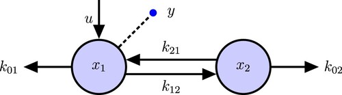
4. 2-Compartment model example

SI analysis of a simple 2-compartment model (Figure 2) demonstrates all of the steps in our new algorithm. (4) $\begin{array}{rl}{\dot{x}}_1& =-(k_{01}+k_{21})x_1+k_{12}{x}_2+u,\\ {\dot{x}}_2& =k_{21}{x}_1-(k_{02}+k_{12})x_2,\\ y& =x_1/V_1.\end{array}$(4) We first use GRA and then our algorithm for finding the I/O equations and show that the results are the same. Then we use the Meshkat algorithm [3] for finding identifiable parameters combinations (combos) and reparametrize the model in terms of these combos. There are n = 2 state variables $\{x_1,x_2\}$, m = 1 output equation $y=x_1/v_1$ and Neq = 3, Nx = 4. Then, according to the GRA Algorithm, taking derivatives $n-(m-1)=2-(1-1)=2$ times is sufficient to find the input–output equation.

Figure 2. 2-Compartmental ODE Model. u is the input to compartment $x_1$, the dashed line with a circle is the output inform compartment $x_2$. The same notation will be used in the following figures.

1: We first differentiate $x_1-V_{1}y$ (output equation) and then add the result to the system (Neq = 4, Nx = 4): (5) ${\dot{x}}_1-V_1\dot{y},$(5)

2: Differentiate ${\dot{x}}_1-V_1\dot{y}$ to obtain $\ddot{y}$, and the corresponding state variable equation to obtain $\ddot{x_1}$ and then add the result to the system (Neq = 6, Nx = 5): (6) $\begin{array}{rl}{\ddot{x}}_1& -V_1\ddot{y},\\ -{\ddot{x}}_1& -(k_{01}+k_{21}){\dot{x}}_1+k_{12}{\dot{x}}_2+\dot{u},\end{array}$(6) The new system has 6 equations in 5 unknown state variables and their derivatives, $\{x_1,x_2,{\dot{x}}_1,{\dot{x}}_2,{\ddot{x}}_1\}$, enough to eliminate all unknowns. According to the GRA algorithm and the ranking $\{{\ddot{x}}_1,{\dot{x}}_2,{\dot{x}}_1,x_2,x_1,\ddot{y},\dot{y},\dot{u},y,u\}$, we find the Gröbner basis of it using Mathematica.Then I/O equation is an equation only in $\{\ddot{y},\dot{y},\dot{u},y,u\}$ of the following form: (7) $\begin{array}{rl}& -(k_{02}+k_{12})u+(k_{01}{k}_{02}+k_{01}{k}_{12}+k_{02}{k}_{21})V_{1}y\\ & -\dot{u}+(k_{01}+k_{02}+k_{12}+k_{21})V_1\dot{y}+V_1\ddot{y}=0,\end{array}$(7) The coefficient matrix for model (4(4) $\begin{array}{rl}{\dot{x}}_1& =-(k_{01}+k_{21})x_1+k_{12}{x}_2+u,\\ {\dot{x}}_2& =k_{21}{x}_1-(k_{02}+k_{12})x_2,\\ y& =x_1/V_1.\end{array}$(4) ) is the following form:

we now use Gaussian elimination on this coefficient matrix and obtain the following matrix in the reduced row-echelon form:

We select the rows of the new matrix which all elements corresponding to state variables and their derivatives are 0 (zero). Multiplying these rows with variables, we obtain the I/O equations (Figures 3 and 4).

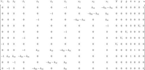
Figure 3. Coefficient matrix of 2-compartment model.

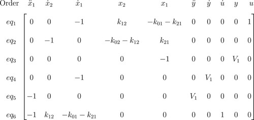
Figure 4. Reduced row-echelon form of 2-compartment model. The last row shows the coefficients of the I/O equations of this model.

The I/O equation for model (4(4) $\begin{array}{rl}{\dot{x}}_1& =-(k_{01}+k_{21})x_1+k_{12}{x}_2+u,\\ {\dot{x}}_2& =k_{21}{x}_1-(k_{02}+k_{12})x_2,\\ y& =x_1/V_1.\end{array}$(4) ) is: (8) $\begin{array}{rl}& -\frac{(k_{02}+k_{12})}{V_1}u+(k_{01}{k}_{02}+k_{01}{k}_{12}+k_{02}{k}_{21})y\\ & -\frac{1}{V_1}\dot{u}+(k_{01}+k_{02}+k_{12}+k_{21})\dot{y}+\ddot{y}=0,\end{array}$(8) Multiplying Equation (8(8) $\begin{array}{rl}& -\frac{(k_{02}+k_{12})}{V_1}u+(k_{01}{k}_{02}+k_{01}{k}_{12}+k_{02}{k}_{21})y\\ & -\frac{1}{V_1}\dot{u}+(k_{01}+k_{02}+k_{12}+k_{21})\dot{y}+\ddot{y}=0,\end{array}$(8) ) by $V_1$, we see our I/O equation is to the same as the GRA algorithm I/O Equation (7(7) $\begin{array}{rl}& -(k_{02}+k_{12})u+(k_{01}{k}_{02}+k_{01}{k}_{12}+k_{02}{k}_{21})V_{1}y\\ & -\dot{u}+(k_{01}+k_{02}+k_{12}+k_{21})V_1\dot{y}+V_1\ddot{y}=0,\end{array}$(7) ). Now we investigate the parameter identifiability of the system (4(4) $\begin{array}{rl}{\dot{x}}_1& =-(k_{01}+k_{21})x_1+k_{12}{x}_2+u,\\ {\dot{x}}_2& =k_{21}{x}_1-(k_{02}+k_{12})x_2,\\ y& =x_1/V_1.\end{array}$(4) ) using Gröbner bases for the solutions to $c(p)=c(p^{\ast })$ and show $V_1,k_{12}{k}_{21},-k_{02}-k_{12},-k_{01}-k_{21}$ are uniquely identifiable. Finally, the most appropriate identifiable combinations are $\{q_1=-k_{01}-k_{21},q_2=k_{12}{k}_{21},q_3=-k_{02}-k_{12},q_4=V_1\}$. Let $x_2=k_{21}{X}_2$. Then the reparameterized equations are: (9) $\begin{array}{rl}{\dot{x}}_1& =q_1{x}_1+q_2{X}_2+u,\\ {\dot{X}}_2& =x_1+q_3{X}_2,y=x_1/q_4.\end{array}$(9)

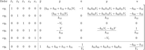
5. 3-Compartment model example

We analyse the 3-compartment model with one output equation shown in Figure 5, to show that we cannot find I/O equations when the number of equations (Neq) is equal to the number of state variables and their derivative (Nx). (10) $\begin{array}{rl}{\dot{x}}_1& =-(k_{21}+k_{31})x_1+k_{12}{x}_2+k_{13}{x}_3+u,\\ {\dot{x}}_2& =k_{21}{x}_1-(k_{02}+k_{12})x_2,\\ {\dot{x}}_3& =k_{31}{x}_1-(k_{03}+k_{13})x_3,\\ y& =x_1/V_1.\end{array}$(10)

Figure 5. 3-Compartment model.

Here we have n = 3 state variables $\{x_1,x_2,x_3\}$, m = 1 output equation $y=x_1/v_1$ and Neq=4, Nx = 6. Then, according to the GRA Algorithm, taking derivatives $n-(m-1)=3-(1-1)=3$ times is sufficient to find the input–output equation.

1: Differentiate $x_1-V_{1}y$ and then add the result to the system (Neq = 5, Nx = 6): (11) ${\dot{x}}_1-V_1\dot{y},$(11)

2: Differentiate ${\dot{x}}_1-V_1\dot{y}$ to obtain $\ddot{y}$, and the corresponding state variable equation to obtain $\ddot{x_1}$ and then add the result to the system (Neq=7, Nx=7): (12) $\begin{array}{rl}{\ddot{x}}_1& -V_1\ddot{y},\\ -{\ddot{x}}_1& -(k_{21}+k_{31}){\dot{x}}_1+k_{12}{\dot{x}}_2+k_{13}{\dot{x}}_3+\dot{u},\end{array}$(12) The new system now has 7 equations in 7 unknown state variables and their derivatives.

3: Differentiate ${\ddot{x}}_1-V_1\ddot{y}$ to obtain $\stackrel{⃛}{y}$, and the corresponding state variable equation to obtain $\stackrel{⃛}{x_1}$, $\ddot{x_2}$ and $\ddot{x_3}$. Then add the result to the system (Neq = 11, Nx = 10): (13) $\begin{array}{rl}{\stackrel{⃛}{x}}_1& -V_1\stackrel{⃛}{y},\\ -{\stackrel{⃛}{x}}_1& -(k_{21}+k_{31}){\ddot{x}}_1+k_{12}{\ddot{x}}_2+k_{13}{\ddot{x}}_3+\ddot{u},\\ -{\ddot{x}}_2& +k_{21}{\dot{x}}_1-(k_{02}+k_{12}){\dot{x}}_2,\\ -{\ddot{x}}_3& +k_{31}{\dot{x}}_1-(k_{03}+k_{13}){\dot{x}}_3,\end{array}$(13) The new system now has 11 equations in 10 unknown state variables and their derivatives, $\{x_1,x_2,x_3,{\dot{x}}_1,{\dot{x}}_2,{\dot{x}}_3,{\ddot{x}}_1,{\ddot{x}}_2,{\ddot{x}}_3,{\stackrel{⃛}{x}}_1\}$, enough to eliminate all unknowns. According to the GRA algorithm and the ranking $\{{\stackrel{⃛}{x}}_1,{\ddot{x}}_3,{\ddot{x}}_2,{\ddot{x}}_1,{\dot{x}}_3,{\dot{x}}_2,{\dot{x}}_1,x_3,x_2,x_1,\stackrel{⃛}{y},\ddot{y},\dot{y},\ddot{u},\dot{u},y,u\}$, we find the Gröbner Basis of it using Mathematica.Then I/O equation is: (14) $\begin{array}{rl}& -(k_{02}{k}_{03}+k_{03}{k}_{12}+k_{02}{k}_{13}+k_{12}{k}_{13})u+(k_{02}{k}_{03}{k}_{21}\\ & +k_{02}{k}_{13}{k}_{21}+k_{02}{k}_{03}{k}_{31}+k_{03}{k}_{12}{k}_{31})V_{1}y\\ & -(k_{02}+k_{03}+k_{12}+k_{13})\dot{u}-\ddot{u}+(k_{02}{k}_{03}+k_{03}{k}_{12}\\ & +k_{02}{k}_{13}+k_{12}{k}_{13}+k_{02}{k}_{21}+k_{03}{k}_{21}+k_{13}{k}_{21}\\ & +k_{02}{k}_{31}+k_{03}{k}_{31}+k_{12}{k}_{31})V_1\dot{y}\\ & +(k_{02}+k_{03}+k_{12}+k_{13}+k_{21}+k_{31})V_1\ddot{y}+V_1\stackrel{⃛}{y}=0\end{array}$(14) The coefficient matrix for (10(10) $\begin{array}{rl}{\dot{x}}_1& =-(k_{21}+k_{31})x_1+k_{12}{x}_2+k_{13}{x}_3+u,\\ {\dot{x}}_2& =k_{21}{x}_1-(k_{02}+k_{12})x_2,\\ {\dot{x}}_3& =k_{31}{x}_1-(k_{03}+k_{13})x_3,\\ y& =x_1/V_1.\end{array}$(10) ) is then:

We then use Gaussian elimination on this matrix and obtain a reduced row echelon form (not shown, too large). We select the only row with zero elements corresponding state variables and their derivatives (Figure 6). (15) $\begin{array}{rl}& \{0,0,0,0,0,0,0,0,0,0,1,k_{02}+k_{03}+k_{12}+k_{13}\\ & +k_{21}+k_{31},k_{02}{k}_{03}+k_{03}{k}_{12}+k_{02}{k}_{13}\\ & +k_{12}{k}_{13}+k_{02}{k}_{21}+k_{03}{k}_{21}+k_{13}{k}_{21}\\ & +k_{02}{k}_{31}+k_{03}{k}_{31}+k_{12}{k}_{31},-(1/V_1),\\ & (-k_{02}-k_{03}-k_{12}-k_{13})/V_1,k_{02}{k}_{03}{k}_{21}\\ & +k_{02}{k}_{13}{k}_{21}+k_{02}{k}_{03}{k}_{31}+k_{03}{k}_{12}{k}_{31},\\ & (-k_{02}{k}_{03}-k_{03}{k}_{12}-k_{02}{k}_{13}-k_{12}{k}_{13})/V_1\}\end{array}$(15) Multiplying this row with variables, we obtain the I/O equation. This equation is the same as that obtained with the GRA algorithm (14(14) $\begin{array}{rl}& -(k_{02}{k}_{03}+k_{03}{k}_{12}+k_{02}{k}_{13}+k_{12}{k}_{13})u+(k_{02}{k}_{03}{k}_{21}\\ & +k_{02}{k}_{13}{k}_{21}+k_{02}{k}_{03}{k}_{31}+k_{03}{k}_{12}{k}_{31})V_{1}y\\ & -(k_{02}+k_{03}+k_{12}+k_{13})\dot{u}-\ddot{u}+(k_{02}{k}_{03}+k_{03}{k}_{12}\\ & +k_{02}{k}_{13}+k_{12}{k}_{13}+k_{02}{k}_{21}+k_{03}{k}_{21}+k_{13}{k}_{21}\\ & +k_{02}{k}_{31}+k_{03}{k}_{31}+k_{12}{k}_{31})V_1\dot{y}\\ & +(k_{02}+k_{03}+k_{12}+k_{13}+k_{21}+k_{31})V_1\ddot{y}+V_1\stackrel{⃛}{y}=0\end{array}$(14) ), after multiplying by $V_1$.

Figure 6. Coefficient matrix of 3-compartment model.

We then use Gröbner bases to find the solutions to $c(p)=c(p^{\ast })$ and show $V_1,k_{21}+k_{31}$ are uniquely identifiable and $k_{02}+k_{12},k_{03}+k_{13},k_{12}{k}_{21},k_{13}{k}_{31}$ are locally identifiable with 2 (two) solutions. Finally, the simplest identifiable combinations $\{q_1=-k_{21}-k_{31},q_2=k_{12}{k}_{21},q_3=k_{13}{k}_{31},q_4=-k_{02}-k_{12},q_5=-k_{03}-k_{13},q_6=V_1\}$ are choosen so all model terms are positive after reparametrizing. Let $x_2=k_{21}{X}_2,x_3=k_{31}{X}_3$. Then the reparameterized equations are: (16) $\begin{array}{rl}{\dot{x}}_1& =q_1{x}_1+q_2{X}_2+q_3{X}_3+u,\\ {\dot{X}}_2& =x_1+q_4{X}_2,\\ {\dot{X}}_3& =x_1+q_5{X}_3,\\ y& =x_1/q_6.\end{array}$(16)

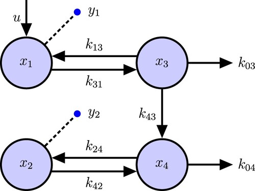
6. 4-Compartment thyroid system model example

The model shown in Figure 7, which represents the linear dynamics of two thyroid hormones (T3 and T4) in blood (1 and 2) and tissues (3 and 4), with conversion of T4 into T3 in the lumped tissue compartment. It has one input and two output. For this example, we find sufficient input–output equations for finding identifiable combinations, with fewer derivatives than with the GRA algorithm. (17) $\begin{array}{rl}{\dot{x}}_1& =-k_{31}{x}_1+k_{13}{x}_3+u,\\ {\dot{x}}_2& =-k_{42}{x}_2+k_{24}{x}_4,\\ {\dot{x}}_3& =k_{31}{x}_1-(k_{03}+k_{13}+k_{43})x_3,\\ {\dot{x}}_4& =k_{42}{x}_2+k_{43}{x}_3-(k_{04}+k_{24})x_4,\\ y_1& =x_1,\\ y_2& =x_2.\end{array}$(17) We use the same method as above, but the minimum bound for the number of taking derivatives is 2 using our algorithm, while it is 3 in GRA algorithm. There are n = 4 state variables $\{x_1,x_2,x_3,x_4\}$ and m = 2 output equations $\{y_1=x_1,y_2=x_2\}$. Then, according to Meshkat [14], taking derivatives $n-(m-1)=4-(2-1)=3$ times is sufficient for finding the I/O equation.

Figure 7. 4-Compartment model.

1: Differentiate $y_1-x_1,y_2-x_2$ (output equations) and then add the result to the system (Neq=8, Nx=8): (18) $\begin{array}{rl}{\dot{y}}_1& -{\dot{x}}_1,\\ {\dot{y}}_2& -{\dot{x}}_2,\end{array}$(18) The number of equations is still not enough to eliminate all unknowns.

2: Differentiate $\dot{y_1}$ and $\dot{y_2}$ to obtain $\ddot{y_1}$ and $\ddot{y_2}$, and the corresponding state variable equation to obtain $\ddot{x_1}$ and $\ddot{x_2}$. Then add the result to the system (Neq=12, Nx=10): (19) $\begin{array}{rl}{\ddot{y}}_1& -{\ddot{x}}_1,\\ {\ddot{y}}_2& -{\ddot{x}}_2,\\ -{\ddot{x}}_1& -k_{31}{\dot{x}}_1+k_{13}{\dot{x}}_3+u,\\ -{\ddot{x}}_2& -k_{42}{\dot{x}}_2+k_{24}{\dot{x}}_4,\end{array}$(19) Then new system now has 12 equations in 10 unknown state variables and their derivatives, $\{x_1,x_2,x_3,x_4,{\dot{x}}_1,{\dot{x}}_2,{\dot{x}}_3,{\dot{x}}_4,{\ddot{x}}_1,{\ddot{x}}_2\}$, enough to eliminate all unknowns. So, we do not need to take another derivative and the algorithm terminates here. According to the GRA algorithm and the ranking $\{{\ddot{x}}_2,{\ddot{x}}_1,{\dot{x}}_4,{\dot{x}}_3,{\dot{x}}_2,{\dot{x}}_1,x_4,x_3,x_2,x_1,{\ddot{y}}_2,{\ddot{y}}_1,{\dot{y}}_2,{\dot{y}}_1,\dot{u},y_2,y_1,u\}$, we find the Gröbner Basis of it using Mathematica.Then I/O equations have the following forms: (20) $\begin{array}{rl}1)& k_{24}{k}_{43}u-k_{24}{k}_{31}{k}_{43}{y}_1+k_{04}{k}_{13}{k}_{42}{y}_2-k_{24}{k}_{43}{\dot{y}}_1\\ & +(k_{04}{k}_{13}+k_{13}{k}_{24}+k_{13}{k}_{42}){\dot{y}}_2+k_{13}{\ddot{y}}_2=0\\ 2)& -(k_{03}+k_{13}+k_{43})u+(k_{03}{k}_{31}+k_{31}{k}_{43})y_1-\dot{u}\\ & +(k_{03}+k_{13}+k_{31}+k_{43})\dot{y_1}+\ddot{y_1}=0\end{array}$(20) Coefficient matrix for model (17(17) $\begin{array}{rl}{\dot{x}}_1& =-k_{31}{x}_1+k_{13}{x}_3+u,\\ {\dot{x}}_2& =-k_{42}{x}_2+k_{24}{x}_4,\\ {\dot{x}}_3& =k_{31}{x}_1-(k_{03}+k_{13}+k_{43})x_3,\\ {\dot{x}}_4& =k_{42}{x}_2+k_{43}{x}_3-(k_{04}+k_{24})x_4,\\ y_1& =x_1,\\ y_2& =x_2.\end{array}$(17) ) is:

We then use Gaussian elimination and acquire a reduced row-echelon form (not shown, too big). We select two rows with 0 (zero) elements corresponding to state variables and their derivatives (Figure 8). $\begin{array}{rl}& 1)\{0,0,0,0,0,0,0,0,0,0,1,0,k_{04}+k_{24}+k_{42},\\ & --{\displaystyle \frac{k_{24}{k}_{43}}{k_{13}}},0,k_{04}{k}_{42},-{\displaystyle \frac{k_{24}{k}_{31}{k}_{43}}{k_{13}}},{\displaystyle \frac{k_{24}{k}_{43}}{k_{13}}}\}\\ & 2)\{0,0,0,0,0,0,0,0,0,0,0,1,0,k_{03}+k_{13}+k_{31}\\ & +k_{43},-1,0,k_{03}{k}_{31}+k_{31}{k}_{43},-k_{03}-k_{13}-k_{43}\}\end{array}$ Multiplying these rows with variables, we obtain two I/O equations: $\begin{array}{rl}& 1)\frac{k_{24}{k}_{43}}{k_{13}}u-\frac{k_{24}{k}_{31}{k}_{43}}{k_{13}}{y}_1+k_{04}{k}_{42}{y}_2-{\displaystyle \frac{k_{24}{k}_{43}}{k_{13}}}{\dot{y}}_1\\ & +(k_{04}+k_{24}+k_{42}){\dot{y}}_2+{\ddot{y}}_2=0\\ & 2)-(k_{03}+k_{13}+k_{43})u+(k_{03}{k}_{31}+k_{31}{k}_{43})y_1\\ & -\dot{u}+(k_{03}+k_{13}+k_{31}+k_{43})\dot{y_1}+\ddot{y_1}=0\end{array}$ Our input–output equations are the same as GRA algorithm I/O Equation (20(20) $\begin{array}{rl}1)& k_{24}{k}_{43}u-k_{24}{k}_{31}{k}_{43}{y}_1+k_{04}{k}_{13}{k}_{42}{y}_2-k_{24}{k}_{43}{\dot{y}}_1\\ & +(k_{04}{k}_{13}+k_{13}{k}_{24}+k_{13}{k}_{42}){\dot{y}}_2+k_{13}{\ddot{y}}_2=0\\ 2)& -(k_{03}+k_{13}+k_{43})u+(k_{03}{k}_{31}+k_{31}{k}_{43})y_1-\dot{u}\\ & +(k_{03}+k_{13}+k_{31}+k_{43})\dot{y_1}+\ddot{y_1}=0\end{array}$(20) ). Finally, we investigate parameter identifiability of the system (17(17) $\begin{array}{rl}{\dot{x}}_1& =-k_{31}{x}_1+k_{13}{x}_3+u,\\ {\dot{x}}_2& =-k_{42}{x}_2+k_{24}{x}_4,\\ {\dot{x}}_3& =k_{31}{x}_1-(k_{03}+k_{13}+k_{43})x_3,\\ {\dot{x}}_4& =k_{42}{x}_2+k_{43}{x}_3-(k_{04}+k_{24})x_4,\\ y_1& =x_1,\\ y_2& =x_2.\end{array}$(17) ) using Gröbner bases for solutions to $c(p)=c(p^{\ast })$ and show $k_{13},k_{31},k_{03}+k_{43},k_{04}{k}_{42},k_{24}{k}_{43}$ and $k_{04}+k_{24}+k_{42}$ are uniquely identifiable.

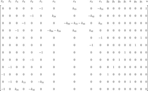
Figure 8. Coefficient matrix of 4-compartmental model.

7. Evaluation of the third derivative

We investigate the result of obtaining a third derivative using the GRA algorithm. we show that the third derivative gives more input–output equations and, consequently, more coefficients. But identifiable parameters combination results are the same as using the Meshkat alghorithm [3].

Let's explore the relationships among the coefficients of the I/O equations obtained from the third and second steps, which do not change the results. A coefficient table of these input–output equations for the second derivative are:

We did not repeat the same coefficients because they do not affect the exhaustive summary or the Gröbner Basis.

For the third derivative, we differentiate $\ddot{y_1}$ and $\ddot{y_2}$ to obtain $\stackrel{⃛}{y_1}$ and $\stackrel{⃛}{y_2}$, and the corresponding state variable equation to acquire $\stackrel{⃛}{x_1}$, $\stackrel{⃛}{x_2}$, $\ddot{x_3}$ and $\ddot{x_4}$. Add these to the system (Neq = 18, Nx = 14): (21) $\begin{array}{rl}{\stackrel{⃛}{y}}_1& -{\stackrel{⃛}{x}}_1,\\ {\stackrel{⃛}{y}}_2& -{\stackrel{⃛}{x}}_2,\\ -{\stackrel{⃛}{x}}_1& -k_{31}{\ddot{x}}_1+k_{13}{\ddot{x}}_3+u,\\ -{\stackrel{⃛}{x}}_2& -k_{42}{\ddot{x}}_2+k_{24}{\ddot{x}}_4,\\ -{\ddot{x}}_3& +k_{31}{\dot{x}}_1-(k_{03}+k_{13}+k_{43}){\dot{x}}_3,\\ -{\ddot{x}}_4& +k_{42}{\dot{x}}_2+k_{43}{\dot{x}}_3-(k_{04}+k_{24}){\dot{x}}_4,\end{array}$(21) Using the GRA algorithm and according to the ranking $\{{\stackrel{⃛}{x}}_2,{\stackrel{⃛}{x}}_1,{\ddot{x}}_4,{\ddot{x}}_3,{\ddot{x}}_2,{\ddot{x}}_1,{\dot{x}}_4,{\dot{x}}_3,{\dot{x}}_2,{\dot{x}}_1,x_4,x_3,x_2,x_1,\stackrel{⃛}{y_2},\stackrel{⃛}{y_1},\ddot{y_2},\ddot{y_1},\dot{y_2},\dot{y_1},\ddot{u},\dot{u},y_2,y_1,u\}$, we find the Gröbner Basis of the new system.Then I/O equations are: (22) $\begin{array}{rl}& 1)k_{24}{k}_{43}u-k_{24}{k}_{31}{k}_{43}{y}_1+k_{04}{k}_{13}{k}_{42}{y}_2-k_{24}{k}_{43}{\dot{y}}_1\\ & +(k_{04}{k}_{13}+k_{13}{k}_{24}+k_{13}{k}_{42}){\dot{y}}_2+k_{13}{\ddot{y}}_2=0\\ & 2)-(k_{03}+k_{13}+k_{43})u+(k_{03}{k}_{31}+k_{31}{k}_{43})y_1\\ & -\dot{u}+(k_{03}+k_{13}+k_{31}+k_{43})\dot{y_1}+\ddot{y_1}=0\\ & 3)(k_{03}^2+2k_{03}{k}_{13}+k_{13}^2+k_{03}{k}_{31}+k_{13}{k}_{31}+2k_{03}{k}_{43}\\ & +2k_{13}{k}_{43}+k_{31}{k}_{43}+k_{43}^2)u\\ & -(k_{03}^2{k}_{31}+k_{03}{k}_{13}{k}_{31}+k_{03}{k}_{31}^2+2k_{03}{k}_{31}{k}_{43}\\ & +k_{13}{k}_{31}{k}_{43}+k_{31}^2{k}_{43}+k_{31}{k}_{43}^2)y_1+k_{31}\dot{u}-\ddot{u}\\ & -(k_{03}^2+2k_{03}{k}_{13}+k_{13}^2+k_{03}{k}_{31}+2k_{13}{k}_{31}\\ & +k_{31}^2+2k_{03}{k}_{43}+2k_{13}{k}_{43}+k_{31}{k}_{43}\\ & +k_{43}^2)\dot{y_1}+\ddot{y_1}=0\\ & 4)-(k_{24}{k}_{43})u+(k_{03}{k}_{04}{k}_{42}+k_{04}{k}_{42}{k}_{43})y_2\\ & +(k_{24}{k}_{43}){\dot{y}}_1+(k_{03}{k}_{04}+k_{03}{k}_{24}+k_{03}{k}_{42}+k_{04}{k}_{42}\\ & +k_{04}{k}_{43}+k_{24}{k}_{43}+k_{42}{k}_{43}){\dot{y}}_2+(k_{03}+k_{04}\\ & +k_{24}+k_{42}+k_{43}){\ddot{y}}_2+{\stackrel{⃛}{y}}_2=0\end{array}$(22) Here we summarize some differences in the procedure of finding identifiable parameter combinations using the second and third derivative. For the second derivative, we have equations (Neq = 12) and state variables and their derivatives (Nx = 10), while for three, Neq=18, Nx=14. Because of this, use of the Grbner Basis or other methods becomes more computationally complex. Also we have 2 (two) input–output equations after two differentiations., After three, we have 4 input–output equations two of which are the same as after two differentiations. The two other input–output equations do not effect the final answer and can be eliminated. We should show that eliminating their coefficient does not effect the exhaustive summary and Grbner Basis. We use a coefficient table of input–output equations, where we write distinct coefficients, because repeating a coefficient does not effect the exhaustive summary and Grbner Basis.

Theorem 7.1

Let $a_1,a_2,\dots ,a_n,b_1,b_2,\dots ,b_m,p_1,p_2,\dots ,p_{n+m}\in \mathbb{R}-\{0\}$, and $n,m\in \mathbb{N}$, then solution set, $\{a_1{a}_2\cdots a_n{b}_1{b}_2\cdots b_m=p_1{p}_2\cdots p_{n+m},a_1=p_1,a_2=p_2,\dots ,a_n=p_n\}$ is equal to solution set, $\{b_1{b}_2\cdots b_m=p_{n+1}{p}_{n+2}\cdots p_{n+m},a_1=p_1,a_2=p_2,\dots ,a_n=p_n\}$. $\begin{array}{rl}& \{\begin{array}{l}{a}_1{a}_2\cdots a_n{b}_1{b}_2\cdots b_m=p_1{p}_2\cdots p_{n+m}\\ a_1=p_1\\ a_2=p_2\\ ⋮\\ a_n=p_n\end{array}\\ & ⟺\{\begin{array}{l}{b}_1{b}_2\cdots b_m=p_{n+1}{p}_{n+2}\cdots p_{n+m}\\ a_1=p_1\\ a_2=p_2\\ ⋮\\ a_n=p_n\end{array}\end{array}$

Proof.

By induction.

Theorem 7.2

Let $a_1,a_2,\dots ,a_n,b_1,b_2,\dots ,b_m,p_1,p_2,\dots ,p_{n+m}\in \mathbb{R}-\{0\}$, and $n,m\in \mathbb{N}$, then solution set, $\{a_1+a_2+\cdots +a_n+b_1+b_2+\cdots +b_m=p_1+p_2+\cdots +p_{n+m},a_1=p_1,a_2=p_2,\dots ,a_n=p_n\}$ is equal to solution set, $\{b_1+b_2+\cdots +b_m=p_{n+1}+p_{n+2}+\cdots +p_{n+m},a_1=p_1,a_2=p_2,\dots ,a_n=p_n\}$. $\begin{array}{rl}& \{\begin{array}{l}{a}_1+a_2+\cdots +a_n+b_1+b_2+\cdots +b_m\\ =p_1+p_2+\cdots +p_{n+m}\\ a_1=p_1\\ a_2=p_2\\ ⋮\\ a_n=p_n\end{array}\\ & \{\begin{array}{l}{b}_1+b_2+\cdots +b_m=p_{n+1}+p_{n+2}+\cdots +p_{n+m}\\ a_1=p_1\\ a_2=p_2\\ ⋮\\ a_n=p_n\end{array}\end{array}$

Proof.

By induction.

Theorem 7.3

Let A, B and C be subsets of the exhaustive summary in linear model, if $A\cup B=C$ and $A\cong A^{\mathrm{\prime }},B\cong B^{\mathrm{\prime }}$, then $C\cong C^{\mathrm{\prime }}=A^{\mathrm{\prime }}\cup B^{\mathrm{\prime }}$ (The symbol ≅ means that two sets have the same distinct solutions).

Proof.

Let $S_A,S_{A^{\mathrm{\prime }}},S_B,S_{B^{\mathrm{\prime }}},S_C$ and $S_{C^{\mathrm{\prime }}}$ denote the sets of solutions of $A,A^{\mathrm{\prime }},B,B^{\mathrm{\prime }},C$ and $C^{\mathrm{\prime }}$ respectively. We should show $S_C\subseteq S_{C^{\mathrm{\prime }}}$ and $S_C\supseteq S_{C^{\mathrm{\prime }}}$. For $S_C\subseteq S_{C^{\mathrm{\prime }}}$, Suppose $s\in S_C=S_A\cup S_B$. Then $s\in S_A$ or $s\in S_B$; if it is in $S_A$, then by relation $A\cong A^{\mathrm{\prime }}$, we have $s\in S_{A^{\mathrm{\prime }}}\subseteq S_{C^{\mathrm{\prime }}}⟹S_C\subseteq S_{C^{\mathrm{\prime }}}$, by symmetry $s\in S_B$ leads to the same conclusion. We also can show $S_C\supseteq S_{C^{\mathrm{\prime }}}$ by using this method.

Theorems 7.1, 7.2 and 7.3 are true for Gröbner Basis of the same model, that is, we can perform Gröbner Basis on each side of above expressions without changing the equality [23]. For theorem 7.1, we need to get the coefficient domain of polynomials as rational functions instead of integers numbers to simplify the solutions. We use these theorems for comparing between the obtained coefficients of I/O equations by taking derivatives two times (Table 1) and three times (Table 2).

Table 1. Coefficients of the I/O Equations for the second derivative.

Coefficients of the I/O Equations ($T_1$)
Coefficients	No. in $T_2$	No. in $T_1$
1	1	1
$k_{13}$	2	2
$k_{24}{k}_{43}$	4	3
$k_{04}{k}_{13}{k}_{42}$	5	4
$k_{24}{k}_{31}{k}_{43}$	6	5
$k_{03}{k}_{31}+k_{31}{k}_{43}$	7	6
$k_{03}+k_{13}+k_{43}$	8	7
$k_{04}{k}_{13}+k_{13}{k}_{24}+k_{13}{k}_{42}$	10	8
$k_{03}+k_{13}+k_{31}+k_{43}$	11	9

Note: No. in $T_1$ is the position of the coefficient in Table 1, No. in $T_2$ is the position of the coefficient in Table 2.

Table 2. Coefficients of the I/O Equations for the third derivative.

Coefficients of the I/O Equations ($T_2$)
Coefficients	No. in $T_2$	RNo.
1	1	1
$k_{13}$	2	2
$k_{31}$	3	3,4
$k_{24}{k}_{43}$	4	3
$k_{04}{k}_{13}{k}_{42}$	5	4
$k_{24}{k}_{31}{k}_{43}$	6	5
$k_{03}{k}_{31}+k_{31}{k}_{43}$	7	6
$k_{03}+k_{13}+k_{43}$	8	7
$k_{03}{k}_{04}{k}_{42}+k_{04}{k}_{42}{k}_{43}$	9	2,3,7
$k_{04}{k}_{13}+k_{13}{k}_{24}+k_{13}{k}_{42}$	10	8
$k_{03}+k_{13}+k_{31}+k_{43}$	11	9
$k_{03}+k_{04}+k_{24}+k_{42}+k_{43}$	12	2,3,4,8,9
$k_{03}{k}_{04}+k_{03}{k}_{24}+k_{03}{k}_{42}+k_{04}{k}_{42}+k_{04}{k}_{43}+k_{24}{k}_{43}+k_{42}{k}_{43}$	13	2,3,4,8,9
$k_{03}^2+2k_{03}{k}_{13}+k_{13}^2+k_{03}{k}_{31}+k_{13}{k}_{31}+2k_{03}{k}_{43}+2k_{13}{k}_{43}+k_{31}{k}_{43}+k_{43}^2$	14	3,4,9
$k_{03}^2+2k_{03}{k}_{13}+k_{13}^2+k_{03}{k}_{31}+2k_{13}{k}_{31}+k_{31}^2+2k_{03}{k}_{43}+2k_{13}{k}_{43}+k_{31}{k}_{43}+k_{43}^2$	15	2,3,4,9
$k_{03}^2{k}_{31}+k_{03}{k}_{13}{k}_{31}+k_{03}{k}_{31}^2+2k_{03}{k}_{31}{k}_{43}+k_{13}{k}_{31}{k}_{43}+k_{31}^2{k}_{43}+k_{31}{k}_{43}^2$	16	2,3,4,9

Note: RNo. is relation number.

We introduce a method to show the relation between the coefficients in Table 1 ($T_1$) and Table 2 ($T_2$).

First, we specify each coefficient according to its position number in $T_1$ or $T_2$. For example, the relation number of coefficient $k_{03}+k_{13}+k_{43}$ is 7 in $T_1$.

Second, the coefficient in each table may have a different relation number. For example, the relation number of coefficient $k_{03}+k_{13}+k_{31}+k_{43}$ is 9 in $T_1$ and 11 in $T_2$.

Third, Suppose coefficient α is in $T_2$, but not in $T_1$. To find relation number in $T_1$, we find a subset A including α of $T_2$ and a subset B of $T_1$ such that $A\cong B$. that is: $\begin{array}{rl}& \mathrm{If}\alpha \in T_2-T_1\mathrm{\exists }\alpha \in A\subset T_1\mathrm{and}\\ & B\subset T_2\mathrm{Such}\mathrm{that}A\cong B\end{array}$ The relation number of $\alpha \in A$ in $T_1$ is equal to all the relation number of the coefficients in B. For example (23) $\begin{array}{rl}& \{k_{03}+k_{13}+k_{43}(7),k_{13}(2)\}\cong \{k_{03}+k_{43}(2,7),k_{13}(2)\}\\ & \{k_{03}+k_{43}(2,7),k_{24}{k}_{43}(3)\}\\ & \cong \{k_{03}{k}_{04}{k}_{42}+k_{04}{k}_{42}{k}_{43}(2,3,7),k_{24}{k}_{43}(3)\}\end{array}$(23) Then the relation number of $k_{03}{k}_{04}{k}_{42}+k_{04}{k}_{42}{k}_{43}$ is 2, 3, 7 in $T_1$. The relation number is not unique and we use them only to show related coefficients do not effect the final answer and can be eliminated. The best way to find these subsets is to write the coefficients in $T_2$ as a combinations of coefficients in $T_1$. Some of these combinations are in the following forms: (24) $\begin{array}{rl}& k_{03}{k}_{04}+k_{03}{k}_{24}+k_{03}{k}_{42}+k_{04}{k}_{42}+k_{04}{k}_{43}\\ & +k_{24}{k}_{43}+k_{42}{k}_{43}\\ & =(k_{03}+k_{43})(k_{04}+k_{24}+k_{42})+k_{04}{k}_{42}\\ & k_{03}^2+2k_{03}{k}_{13}+k_{13}^2+k_{03}{k}_{31}+k_{13}{k}_{31}+2k_{03}{k}_{43}\\ & +2k_{13}{k}_{43}+k_{31}{k}_{43}+k_{43}^2\\ & =(k_{03}+k_{13}+k_{43})(k_{03}+k_{13}+k_{31}+k_{43})\\ & k_{03}^2+2k_{03}{k}_{13}+k_{13}^2+k_{03}{k}_{31}+2k_{13}{k}_{31}+k_{31}^2\\ & +2k_{03}{k}_{43}+2k_{13}{k}_{43}+k_{31}{k}_{43}+k_{43}^2\\ & =(k_{03}+k_{13}+k_{43})(k_{03}+k_{13}+k_{31}+k_{43})\\ & +k_{31}(k_{13}+k_{31})\\ & k_{03}^2{k}_{31}+k_{03}{k}_{13}{k}_{31}+k_{03}{k}_{31}^2+2k_{03}{k}_{31}{k}_{43}\\ & +k_{13}{k}_{31}{k}_{43}+k_{31}^2{k}_{43}+k_{31}{k}_{43}^2\\ & =k_{31}(k_{03}+k_{43})(k_{03}+k_{13}+k_{31}+k_{43})\end{array}$(24)

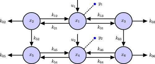
8. Linear thyroid hormone distribution and metabolism (D&M) model example (Figure 9)

This more complex version of a well-studied biosystem model [24–26] illustrates the power of our algorithm. (25) $\begin{array}{rl}{\dot{x}}_1& =k_{12}{x}_2+k_{13}{x}_3-(k_{31}+k_{21})x_1+u_1,\\ {\dot{x}}_2& =k_{21}{x}_1-(k_{12}+k_{02}+k_{52})x_2,\\ {\dot{x}}_3& =k_{31}{x}_1-(k_{13}+k_{03}+k_{63})x_3,\\ {\dot{x}}_4& =k_{45}{x}_5+k_{46}{x}_6-(k_{64}+k_{54})x_4+u_2,\\ {\dot{x}}_5& =k_{54}{x}_4+k_{52}{x}_2-(k_{45}+k_{05})x_5,\\ {\dot{x}}_6& =k_{64}{x}_4+k_{63}{x}_3-(k_{46}+k_{06})x_6,\\ y_1& =x_1,\\ y_2& =x_4.\end{array}$(25) We use the method of Section 4. This model has n = 6 state variables $\{x_1,x_2,x_3,x_4,x_5,x_6\}$ and m = 2 output equations $\{y_1=x_1,y_2=x_4\}$. Then, according to the GRA algorithm, taking derivatives $n-(m-1)=6-(2-1)=5$ times is sufficient to find the input–output equation (Figure 9).

1: We differentiate $y_1-x_1$ and $y_4-x_4$ and then add the result to the system (Neq = 10, Nx = 12): (26) $\begin{array}{rl}{\dot{y}}_1& -{\dot{x}}_1,\\ {\dot{y}}_4& -{\dot{x}}_4,\end{array}$(26)

2: Differentiate $\dot{y_1}$ and $\dot{y_2}$ to obtain $\ddot{y_1}$ and $\ddot{y_2}$, and the corresponding state variable equation to acquire $\ddot{x_1}$ and $\ddot{x_4}$. Add these to the system (Neq = 14, Nx = 14): (27) $\begin{array}{rl}{\ddot{y}}_1& -{\ddot{x}}_1,\\ {\ddot{y}}_4& -{\ddot{x}}_4,\\ -{\ddot{x}}_1& +k_{12}{\dot{x}}_2+k_{13}{\dot{x}}_3-(k_{31}+k_{21}){\dot{x}}_1+{\dot{u}}_1,\\ -{\ddot{x}}_4& +k_{45}{\dot{x}}_5+k_{46}{\dot{x}}_6-(k_{64}+k_{54}){\dot{x}}_4+{\dot{u}}_2,\end{array}$(27)

Figure 9. Linear thyroid D&M model.

3: Differentiate $\ddot{y_1}$ and $\ddot{y_2}$ to obtain $\stackrel{⃛}{y_1}$ and $\stackrel{⃛}{y_2}$, and the corresponding state variable equation to acquire $\stackrel{⃛}{x_1}$, $\stackrel{⃛}{x_4}$, $\ddot{x_3}$ and $\ddot{x_4}$. Add these to the system (Neq=22, Nx=20): (28) $\begin{array}{rl}{\stackrel{⃛}{y}}_1& -{\stackrel{⃛}{x}}_1,\\ {\stackrel{⃛}{y}}_4& -{\stackrel{⃛}{x}}_4,\\ -{\stackrel{⃛}{x}}_1& +k_{12}{\ddot{x}}_2+k_{13}{\ddot{x}}_3-(k_{31}+k_{21}){\ddot{x}}_1+{\ddot{u}}_1,\\ -{\stackrel{⃛}{x}}_4& +k_{45}{\ddot{x}}_5+k_{46}{\ddot{x}}_6-(k_{64}+k_{54}){\ddot{x}}_4+{\ddot{u}}_2,\\ -{\ddot{x}}_2& +k_{21}{\dot{x}}_1-(k_{12}+k_{02}+k_{52}){\dot{x}}_2,\\ -{\ddot{x}}_3& +k_{31}{\dot{x}}_1-(k_{13}+k_{03}+k_{63}){\dot{x}}_3,\\ -{\ddot{x}}_5& +k_{54}{\dot{x}}_4+k_{52}{\dot{x}}_2-(k_{45}+k_{05}){\dot{x}}_5,\\ -{\ddot{x}}_6& +k_{64}{\dot{x}}_4+k_{63}{\dot{x}}_3-(k_{46}+k_{06}){\dot{x}}_6,\end{array}$(28)

The new system now has 22 equations in 20 unknown state variables and their derivatives, $\{x_1,x_2,x_3,x_4,x_5,x_6,{\dot{x}}_1,{\dot{x}}_2,{\dot{x}}_3,{\dot{x}}_4,{\dot{x}}_5,{\dot{x}}_6,{\ddot{x}}_1,{\ddot{x}}_2,{\ddot{x}}_3,{\ddot{x}}_4,{\ddot{x}}_5,{\ddot{x}}_6,{\stackrel{⃛}{x}}_1,{\stackrel{⃛}{x}}_4\}$, enough to eliminate all unknowns. The algorithm terminates here. (In comparison the GRA algorithm requires 5 (instead of 3) steps, giving 38 equations in 32 unknown (instead of 22 in 20 unknowns) state variables and their derivatives). This gives two input–output equations.

To test structural identifiability of this model, we adopt the quasi-numerical method used in DAISY [7]. We provide the exhaustive summary $c(p)$, using coefficients of the I/O equations plus random numbers. For every function of the unknown p in the exhaustive summary we assign a pseudo-randomly chosen numerical value for the elements of vector p, providing a system of nonlinear algebraic equations in the unknown p. This quasi-numerical approach allows significantly reduced symbolic computations and hence broadens the class of testable models. For this example, the resulting nonlinear algebraic equations (with random numbers) were solved using Mathematica, which returns solutions for each unknown parameter. When these solutions indicate that the parameter is equal to its assigned number, the model is globally structurally identifiable, otherwise it is not. We chose numerical parameter values as follows: (29) $\begin{array}{rl}\{& k_{02}\to 2,k_{03}\to 3,k_{05}\to 5,k_{06}\to 7,k_{12}\to 11,\\ & k_{13}\to 13,k_{21}\to 17,k_{31}\to 19,k_{45}\to 23,\\ & k_{46}\to 29,k_{52}\to 31,k_{54}\to 37,k_{63}\to 41,k_{64}\to 43\}\end{array}$(29) After solving exhaustive summary, none are equal to their numerical value, so the model is not structurally identifiable (Appendix 1).

9. Implementation of method as web application

Our new algorithm is implemented as web application COMBOS2, available online at: http://biocyb1.cs.ucla.edu/combos2. To show the speed of our algorithm compared with the Gröbner Basis approach in COMBOS, we give some examples of analyzing linear models for identifiable combinations, which DAISY does not provide. COMBOS [8] provides identifiable parameter combinations for the 4-Compartment biosystem model in about 17 seconds, decreasing to 5 seconds with COMBOS2. COMBOS2 shows that a 5-Compartment identifiable model [27] is identifiable in about 9 seconds, whereas COMBOS needs 28 seconds. Each is at least 3 times faster with COMBOS2. For the 6-compartment linear thyroid model above, COMBOS did not provide any answer because it hung during the I/O phase of the computation. COMBOS2 took only 2 seconds for finding I/O equations, but it also hangs when attempting to find identifiable parameter combinations, because it uses the Gröbner Basis approach in its paramter combinations algorithm. An alternative method for solving this problem using Mathematica is described in the Appendix 2. DAISY does not compute identifiable parameters combinations, but it did analyse for structural identifiability of individual parameters, and this took several hours to complete.

10. Conclusion

We introduced a novel algorithm for finding the I/O equations for systems of linear biosystem models and other linear ODEs of the form (1(1) $\begin{array}{rl}\dot{x}(t,\mathbf{p})& =f(x(t,\mathbf{p}),u(t),t;\mathbf{p}),t\in [t_0,T]\\ y(t,\mathbf{p})& =g(x(t,\mathbf{p});\mathbf{p}),\end{array}$(1) ) with m output equations, by taking derivatives of the system and then using a Gaussian elimination approach. The new algorithm runs much faster and is simpler to implement than a Grobner basis approach. We also showed the number of derivatives needed for computing I/O equations is smaller when the condition Neq ≥ Nx + m is satisfied. We demonstated the utility of the new algorithmic approach in a new app COMBOS2, applying it to several example models and, in particular, to a 6-dimensional thyroid hormone dynamics model, shown in 2 seconds to be not structurally identifiable, while COMBOS provided no solution. Another app DASIY needed several hours to provide only a structural identifiability analysis for the original individual parameters, and no parameter combination results. The main limitation of our new algorithm is, of course, that it is not applicable to nonlinear biosystem models. But we believe it gets a bit closer.

Disclosure statement

No potential conflict of interest was reported by the authors.

Notes

1 http://biocyb1.cs.ucla.edu/combos/

2 http://daisy.dei.unipd.it/

Appendices

Appendix 1

(A1) $\begin{array}{rl}& 1)k_{02}\to {\displaystyle \frac{1333k_{63}-51619}{1517}},k_{03}\to 44-k_{63},\\ & k_{05}\to {\displaystyle \frac{1204k_{63}-56949}{43k_{63}-3280}},k_{06}\to {\displaystyle \frac{36k_{63}-1189}{k_{63}}},\\ & k_{12}\to 11,k_{13}\to 13,k_{21}\to 17,k_{31}\to 19,\\ & k_{45}\to -{\displaystyle \frac{34891}{43k_{63}-3280}},k_{46}\to {\displaystyle \frac{1189}{k_{63}}},\\ & k_{52}\to -{\displaystyle \frac{31(43k_{63}-3280)}{1517}},k_{54}\to {\displaystyle \frac{1}{41}}(3280-43k_{63}),\\ & k_{64}\to {\displaystyle \frac{43k_{63}}{41}}\end{array}$(A1) (A2) $\begin{array}{rl}& 2)k_{02}\to {\displaystyle \frac{385237k_{63}-14136513}{547637}},k_{03}\to {\displaystyle \frac{1}{17}}(722-17k_{63}),\\ & k_{05}\to {\displaystyle \frac{20468k_{63}-1082031}{731k_{63}-62320}},\\ & k_{06}\to {\displaystyle \frac{612k_{63}-22591}{17k_{63}}},k_{12}\to {\displaystyle \frac{187}{19}},k_{13}\to {\displaystyle \frac{247}{17}},\\ & k_{21}\to 19,k_{31}\to 17,k_{45}\to -{\displaystyle \frac{662929}{731k_{63}-62320}},\\ & k_{46}\to {\displaystyle \frac{22591}{17k_{63}}},k_{52}\to -{\displaystyle \frac{527(731k_{63}-62320)}{547637}},\\ & k_{54}\to {\displaystyle \frac{1}{779}}(62320-731k_{63}),k_{64}\to {\displaystyle \frac{731k_{63}}{779}},\end{array}$(A2) (A3) $\begin{array}{rl}& 3)k_{02}\to {\displaystyle \frac{\begin{array}{c}54612\sqrt{647}{k}_{63}-1473007k_{63}\\ -2023153\sqrt{647}+58375263\end{array}}{385237}},\\ & k_{03}\to {\displaystyle \frac{1}{19}}(-19k_{63}+11\sqrt{647}+1034),\\ & k_{05}\to -{\displaystyle \frac{38657\sqrt{647}}{({\displaystyle \frac{2480\sqrt{647}}{k_{63}}}+{\displaystyle \frac{44640}{k_{63}}}+703)k_{63}}}\\ & -{\displaystyle \frac{695826}{({\displaystyle \frac{2480\sqrt{647}}{k_{63}}}+{\displaystyle \frac{44640}{k_{63}}}+703)k_{63}}}+36,\\ & k_{06}\to {\displaystyle \frac{532k_{63}+713\sqrt{647}+12834}{19k_{63}}},\\ & k_{12}\to {\displaystyle \frac{13}{17}}(\sqrt{647}-18),k_{13}\to {\displaystyle \frac{11}{19}}(-\sqrt{647}-18),\\ & k_{21}\to \sqrt{647}+18,k_{31}\to 18-\sqrt{647},\\ & k_{45}\to {\displaystyle \frac{38657({\displaystyle \frac{\sqrt{647}}{k_{63}}}+{\displaystyle \frac{18}{k_{63}}})}{{\displaystyle \frac{2480\sqrt{647}}{k_{63}}}+{\displaystyle \frac{44640}{k_{63}}}+703}},\\ & k_{46}\to -{\displaystyle \frac{713(\sqrt{647}+18)}{19k_{63}}},\\ & k_{52}\to -{\displaystyle \frac{\begin{array}{c}41(1332\sqrt{647}{k}_{63}-35927k_{63}\\ -42160\sqrt{647}+758880)\end{array}}{385237}},\\ & k_{54}\to {\displaystyle \frac{1}{527}}(37\sqrt{647}{k}_{63}-666k_{63}+42160),\\ & k_{64}\to {\displaystyle \frac{1}{527}}(-37)(\sqrt{647}{k}_{63}-18k_{63}),\end{array}$(A3) (A4) $\begin{array}{rl}& 4)k_{02}\to {\displaystyle \frac{\begin{array}{c}-54612\sqrt{647}{k}_{63}-1473007k_{63}\\ +2023153\sqrt{647}+58375263\end{array}}{385237}},\\ & k_{03}\to {\displaystyle \frac{1}{19}}(-19k_{63}-11\sqrt{647}+1034),\\ & k_{05}\to -{\displaystyle \frac{38657\sqrt{647}}{({\displaystyle \frac{2480\sqrt{647}}{k_{63}}}-{\displaystyle \frac{44640}{k_{63}}}-703)k_{63}}}\\ & +{\displaystyle \frac{695826}{({\displaystyle \frac{2480\sqrt{647}}{k_{63}}}-{\displaystyle \frac{44640}{k_{63}}}-703)k_{63}}}+36,\\ & k_{06}\to {\displaystyle \frac{532k_{63}-713\sqrt{647}+12834}{19k_{63}}},\\ & k_{12}\to {\displaystyle \frac{13}{17}}(-\sqrt{647}-18),k_{13}\to {\displaystyle \frac{11}{19}}(\sqrt{647}-18),\\ & k_{21}\to 18-\sqrt{647},k_{31}\to \sqrt{647}+18,\\ & k_{45}\to {\displaystyle \frac{38657({\displaystyle \frac{\sqrt{647}}{k_{63}}}-{\displaystyle \frac{18}{k_{63}}})}{{\displaystyle \frac{2480\sqrt{647}}{k_{63}}}-{\displaystyle \frac{44640}{k_{63}}}-703}},\\ & k_{46}\to {\displaystyle \frac{713(\sqrt{647}-18)}{19k_{63}}},\\ & k_{52}\to {\displaystyle \frac{\begin{array}{c}41(1332\sqrt{647}{k}_{63}+35927k_{63}\\ -42160\sqrt{647}-758880)\end{array}}{385237}},\\ & k_{54}\to {\displaystyle \frac{1}{527}}(-37\sqrt{647}{k}_{63}-666k_{63}+42160),\\ & k_{64}\to {\displaystyle \frac{37}{527}}(\sqrt{647}{k}_{63}+18k_{63})\end{array}$(A4)

Appendix 2

In this section, we introduced a method for finding identifiable parameters combinations of the linear thyroid model by using Mathematica. COMBOS2 hangs when attempting to find identifiable parameter combinations. A technique for solving this problem is to reduce the number of parameters by substituting some of them with numbers.

First Step. According to the calculations for the linear thyroid model (A1(A1) $\begin{array}{rl}& 1)k_{02}\to {\displaystyle \frac{1333k_{63}-51619}{1517}},k_{03}\to 44-k_{63},\\ & k_{05}\to {\displaystyle \frac{1204k_{63}-56949}{43k_{63}-3280}},k_{06}\to {\displaystyle \frac{36k_{63}-1189}{k_{63}}},\\ & k_{12}\to 11,k_{13}\to 13,k_{21}\to 17,k_{31}\to 19,\\ & k_{45}\to -{\displaystyle \frac{34891}{43k_{63}-3280}},k_{46}\to {\displaystyle \frac{1189}{k_{63}}},\\ & k_{52}\to -{\displaystyle \frac{31(43k_{63}-3280)}{1517}},k_{54}\to {\displaystyle \frac{1}{41}}(3280-43k_{63}),\\ & k_{64}\to {\displaystyle \frac{43k_{63}}{41}}\end{array}$(A1) ), (A2(A2) $\begin{array}{rl}& 2)k_{02}\to {\displaystyle \frac{385237k_{63}-14136513}{547637}},k_{03}\to {\displaystyle \frac{1}{17}}(722-17k_{63}),\\ & k_{05}\to {\displaystyle \frac{20468k_{63}-1082031}{731k_{63}-62320}},\\ & k_{06}\to {\displaystyle \frac{612k_{63}-22591}{17k_{63}}},k_{12}\to {\displaystyle \frac{187}{19}},k_{13}\to {\displaystyle \frac{247}{17}},\\ & k_{21}\to 19,k_{31}\to 17,k_{45}\to -{\displaystyle \frac{662929}{731k_{63}-62320}},\\ & k_{46}\to {\displaystyle \frac{22591}{17k_{63}}},k_{52}\to -{\displaystyle \frac{527(731k_{63}-62320)}{547637}},\\ & k_{54}\to {\displaystyle \frac{1}{779}}(62320-731k_{63}),k_{64}\to {\displaystyle \frac{731k_{63}}{779}},\end{array}$(A2) ), (A3(A3) $\begin{array}{rl}& 3)k_{02}\to {\displaystyle \frac{\begin{array}{c}54612\sqrt{647}{k}_{63}-1473007k_{63}\\ -2023153\sqrt{647}+58375263\end{array}}{385237}},\\ & k_{03}\to {\displaystyle \frac{1}{19}}(-19k_{63}+11\sqrt{647}+1034),\\ & k_{05}\to -{\displaystyle \frac{38657\sqrt{647}}{({\displaystyle \frac{2480\sqrt{647}}{k_{63}}}+{\displaystyle \frac{44640}{k_{63}}}+703)k_{63}}}\\ & -{\displaystyle \frac{695826}{({\displaystyle \frac{2480\sqrt{647}}{k_{63}}}+{\displaystyle \frac{44640}{k_{63}}}+703)k_{63}}}+36,\\ & k_{06}\to {\displaystyle \frac{532k_{63}+713\sqrt{647}+12834}{19k_{63}}},\\ & k_{12}\to {\displaystyle \frac{13}{17}}(\sqrt{647}-18),k_{13}\to {\displaystyle \frac{11}{19}}(-\sqrt{647}-18),\\ & k_{21}\to \sqrt{647}+18,k_{31}\to 18-\sqrt{647},\\ & k_{45}\to {\displaystyle \frac{38657({\displaystyle \frac{\sqrt{647}}{k_{63}}}+{\displaystyle \frac{18}{k_{63}}})}{{\displaystyle \frac{2480\sqrt{647}}{k_{63}}}+{\displaystyle \frac{44640}{k_{63}}}+703}},\\ & k_{46}\to -{\displaystyle \frac{713(\sqrt{647}+18)}{19k_{63}}},\\ & k_{52}\to -{\displaystyle \frac{\begin{array}{c}41(1332\sqrt{647}{k}_{63}-35927k_{63}\\ -42160\sqrt{647}+758880)\end{array}}{385237}},\\ & k_{54}\to {\displaystyle \frac{1}{527}}(37\sqrt{647}{k}_{63}-666k_{63}+42160),\\ & k_{64}\to {\displaystyle \frac{1}{527}}(-37)(\sqrt{647}{k}_{63}-18k_{63}),\end{array}$(A3) ), (A4(A4) $\begin{array}{rl}& 4)k_{02}\to {\displaystyle \frac{\begin{array}{c}-54612\sqrt{647}{k}_{63}-1473007k_{63}\\ +2023153\sqrt{647}+58375263\end{array}}{385237}},\\ & k_{03}\to {\displaystyle \frac{1}{19}}(-19k_{63}-11\sqrt{647}+1034),\\ & k_{05}\to -{\displaystyle \frac{38657\sqrt{647}}{({\displaystyle \frac{2480\sqrt{647}}{k_{63}}}-{\displaystyle \frac{44640}{k_{63}}}-703)k_{63}}}\\ & +{\displaystyle \frac{695826}{({\displaystyle \frac{2480\sqrt{647}}{k_{63}}}-{\displaystyle \frac{44640}{k_{63}}}-703)k_{63}}}+36,\\ & k_{06}\to {\displaystyle \frac{532k_{63}-713\sqrt{647}+12834}{19k_{63}}},\\ & k_{12}\to {\displaystyle \frac{13}{17}}(-\sqrt{647}-18),k_{13}\to {\displaystyle \frac{11}{19}}(\sqrt{647}-18),\\ & k_{21}\to 18-\sqrt{647},k_{31}\to \sqrt{647}+18,\\ & k_{45}\to {\displaystyle \frac{38657({\displaystyle \frac{\sqrt{647}}{k_{63}}}-{\displaystyle \frac{18}{k_{63}}})}{{\displaystyle \frac{2480\sqrt{647}}{k_{63}}}-{\displaystyle \frac{44640}{k_{63}}}-703}},\\ & k_{46}\to {\displaystyle \frac{713(\sqrt{647}-18)}{19k_{63}}},\\ & k_{52}\to {\displaystyle \frac{\begin{array}{c}41(1332\sqrt{647}{k}_{63}+35927k_{63}\\ -42160\sqrt{647}-758880)\end{array}}{385237}},\\ & k_{54}\to {\displaystyle \frac{1}{527}}(-37\sqrt{647}{k}_{63}-666k_{63}+42160),\\ & k_{64}\to {\displaystyle \frac{37}{527}}(\sqrt{647}{k}_{63}+18k_{63})\end{array}$(A4) ), the best choice is as follows: (A5) $\{k_{12}\to 11,k_{13}\to 13,k_{21}\to 17,k_{31}\to 19\}$(A5) After substituting these parameters in $c(p)=c(p^{\ast })$, we investigate the parameter identifiability of the system (25(25) $\begin{array}{rl}{\dot{x}}_1& =k_{12}{x}_2+k_{13}{x}_3-(k_{31}+k_{21})x_1+u_1,\\ {\dot{x}}_2& =k_{21}{x}_1-(k_{12}+k_{02}+k_{52})x_2,\\ {\dot{x}}_3& =k_{31}{x}_1-(k_{13}+k_{03}+k_{63})x_3,\\ {\dot{x}}_4& =k_{45}{x}_5+k_{46}{x}_6-(k_{64}+k_{54})x_4+u_2,\\ {\dot{x}}_5& =k_{54}{x}_4+k_{52}{x}_2-(k_{45}+k_{05})x_5,\\ {\dot{x}}_6& =k_{64}{x}_4+k_{63}{x}_3-(k_{46}+k_{06})x_6,\\ y_1& =x_1,\\ y_2& =x_4.\end{array}$(25) ) using Gröbner bases for the solutions to new $c(p)=c(p^{\ast })$ and have: (A6) $\begin{array}{rl}& \{k_{54}+k_{64},k_{46}{k}_{64},k_{46}{k}_{63},k_{45}{k}_{64},k_{45}{k}_{52},\\ & k_{06}+k_{46},k_{05}+k_{45},k_{03}+k_{63},k_{02}+k_{52}\}\end{array}$(A6) Let $k_{5464}=k_{54}+k_{64},k_{46T64}=k_{46}{k}_{64},k_{46T63}=k_{46}{k}_{63},k_{45T64}=k_{45}{k}_{64},k_{45T52}=k_{45}{k}_{52},k_{0646}=k_{06}+k_{46},k_{0545}=k_{05}+k_{45},k_{0363}=k_{03}+k_{63},k_{0252}=k_{02}+k_{52}$, and also $X_2=k_{12}{x}_2,X_3=k_{13}{x}_3,X_5=k_{45}{x}_5,X_6=k_{46}{x}_6,k_{45T52T12}=k_{45T52}{k}_{12},k_{46T63T13}=k_{46T63}{k}_{13}$. Then the reparameterized equations are: (A7) $\begin{array}{rl}{\dot{x}}_1& =X_2+X_3-(k_{21}+k_{31})x_1+u_1,\\ {\dot{X}}_2& =k_{12T21}{x}_1-(k_{12}+k_{0252})X_2,\\ {\dot{X}}_3& =k_{13T31}{x}_1-(k_{13}+k_{0363})X_3,\\ {\dot{x}}_4& =X_5+X_6-k_{6454}{x}_4+u_2,\\ {\dot{X}}_5& =k_{45T54}{x}_4+k_{45T52T12}{X}_2-k_{0545}{X}_5,\\ {\dot{X}}_6& =k_{46T64}{x}_4+k_{46T63T13}{X}_3-k_{4606}{X}_6,\\ y_1& =x_1,\\ y_2& =x_4.\end{array}$(A7) Second Step. Using Mathematica we investigate the parameter identifiability of this new system (A7(A7) $\begin{array}{rl}{\dot{x}}_1& =X_2+X_3-(k_{21}+k_{31})x_1+u_1,\\ {\dot{X}}_2& =k_{12T21}{x}_1-(k_{12}+k_{0252})X_2,\\ {\dot{X}}_3& =k_{13T31}{x}_1-(k_{13}+k_{0363})X_3,\\ {\dot{x}}_4& =X_5+X_6-k_{6454}{x}_4+u_2,\\ {\dot{X}}_5& =k_{45T54}{x}_4+k_{45T52T12}{X}_2-k_{0545}{X}_5,\\ {\dot{X}}_6& =k_{46T64}{x}_4+k_{46T63T13}{X}_3-k_{4606}{X}_6,\\ y_1& =x_1,\\ y_2& =x_4.\end{array}$(A7) ) and find the following combinations: (A8) $\begin{array}{rl}& \{k_{5464},k_{46T64},k_{46T63T13},k_{45T54},k_{45T52T12},\\ & k_{4505},k_{21}+k_{31},k_{13T31},k_{12T21},k_{0646},\\ & k_{0363}+k_{13},k_{0252}+k_{12}\}\end{array}$(A8) By combining the identifiabile parameters combinations obtained from the first (A6(A6) $\begin{array}{rl}& \{k_{54}+k_{64},k_{46}{k}_{64},k_{46}{k}_{63},k_{45}{k}_{64},k_{45}{k}_{52},\\ & k_{06}+k_{46},k_{05}+k_{45},k_{03}+k_{63},k_{02}+k_{52}\}\end{array}$(A6) ) and second (A8(A8) $\begin{array}{rl}& \{k_{5464},k_{46T64},k_{46T63T13},k_{45T54},k_{45T52T12},\\ & k_{4505},k_{21}+k_{31},k_{13T31},k_{12T21},k_{0646},\\ & k_{0363}+k_{13},k_{0252}+k_{12}\}\end{array}$(A8) ) steps for the linear thyroid model, we have the following Table 3:

Table A1. The identifiabile parameters combinations of the linear thyroid model.

Uniquely Identifiabile Parameters Combinations for Linear Thyroid Model
$K_{11}=-k_{21}-k_{31}$
$K_{22}=-(k_{0252}+k_{12})=-k_{12}-k_{02}-k_{52}$
$K_{33}=-(k_{0363}+k_{13})=-k_{13}-k_{03}-k_{63}$
$K_{44}=-k_{5464}=-k_{54}-k_{64}$
$K_{55}=-k_{4505}=-k_{45}-k_{05}$
$K_{66}=-k_{4606}=-k_{46}-k_{06}$
$T_{22}=k_{12T21}=k_{12}{k}_{21}$
$T_{33}=k_{13T31}=k_{13}{k}_{31}$
$T_{52}=k_{45T52T12}=k_{45T52}{k}_{12}=k_{45}{k}_{52}{k}_{12}$
$T_{55}=k_{45T54}=k_{45}{k}_{54}$
$T_{63}=k_{46T63T13}=k_{46T63}{k}_{13}=k_{46}{k}_{63}{k}_{13}$
$T_{66}=k_{46T64}=k_{46}{k}_{64}$

Then the reparameterized linear thyroid model equations are: (A9) $\begin{array}{rl}{\dot{x}}_1& =X_2+X_3+K_{11}{x}_1+u_1,\\ {\dot{X}}_2& =T_{22}{x}_1+K_{22}{X}_2,\\ {\dot{X}}_3& =T_{33}{x}_1+K_{33}{X}_3,\\ {\dot{x}}_4& =X_5+X_6+K_{44}{x}_4+u_2,\\ {\dot{X}}_5& =T_{55}{x}_4+T_{52}{X}_2+K_{55}{X}_5,\\ {\dot{X}}_6& =T_{66}{x}_4+T_{63}{X}_3+K_{66}{X}_6,\\ y_1& =x_1,\\ y_2& =x_4.\end{array}$(A9)

References

- DiStefano III J. Dynamic systems biology modeling and simulation. Waltham (MA): Academic Press; 2015; Jan 10.
- Cobelli C, Distefano 3rd JJ. Parameter and structural identifiability concepts and ambiguities: a critical review and analysis. Am J Physiol Regul Integr Comp Physiol. 1980;239(1):R7–R24.
- Meshkat N, Anderson C, DiStefanoIII JJ. Alternative to Ritt's pseudodivision for finding the input-output equations of multi-output models. Math Biosci. 2012;239(1):117–123.
- Ljung L, Glad T. On global identifiability for arbitrary model parametrizations. Automatica. 1994;30(2):265–276.
- Itu C, Ochsner A, Vlase S, et al. Improved rigidity of composite circular plates through radial ribs. Proc Inst Mech Eng Pt L J Mater Des Appl. 2019;233(8):1585–1593.
- Marin M, Craciun EM, Pop N. Considerations on mixed initial-boundary value problems for micropolar porous bodies. Dyn Syst Appl. 2016;25(1–2):175–196.
- Bellu G, Saccomani MP, Audoly S, et al. DAISY: a new software tool to test global identifiability of biological and physiological systems. Comput Methods Programs Biomed. 2007;88(1):52–61.
- Meshkat N, Kuo CE, DiStefano III J. On finding and using identifiable parameter combinations in nonlinear dynamic systems biology models and COMBOS: a novel web implementation. PLoS ONE. 2014;9(10):e110261.
- Ritt JF. Differential algebra. New York (NY): American Mathematical Society; 1950.
- Jirstrand M. Algebraic methods for modeling and design in control. Division of Automatic Control, Department of Electrical Engineering, Linkping University; 1996.
- Yazdi MK. An accurate relationship between frequency and amplitude to nonlinear oscillations. J Taibah Univ Sci. 2018;12(5):532–535.
- Marin M, Vlase S, Ellahi R, et al. On the partition of energies for the backward in time problem of thermoelastic materials with a dipolar structure. Symmetry. 2019;11(7):863.
- Bhatti MM, Shahid A, Abbas T, et al. Study of activation energy on the movement of gyrotactic microorganism in a magnetized nanofluids past a porous plate. Processes. 2020;8(3):328.
- Meshkat N, Eisenberg M, DiStefano III JJ. An algorithm for finding globally identifiable parameter combinations of nonlinear ODE models using Grbner Bases. Math Biosci. 2009;222(2):61–72.
- Meshkat NC. A differential algebra method for eliminating unidentifiability. Los Angeles: University of California; 2011.
- Saccomani MP, Audoly S, Bellu G, et al. Examples of testing global identifiability of biological and biomedical models with the DAISY software. Comput Biol Med. 2010;40(4):402–407.
- Bareiss EH. Sylvester's identity and multistep integer-preserving Gaussian elimination. Math Comput. 1968;22(103):565–578.
- Marin M, Nicaise S. Existence and stability results for thermoelastic dipolar bodies with double porosity. Continuum Mech Thermodyn. 2016;28(6):1645–1657.
- Abbas IA. Eigenvalue approach for an unbounded medium with a spherical cavity based upon two-temperature generalized thermoelastic theory. J Mech Sci Technol. 2014;28(10):4193–4198.
- Marin M, Ellahi R, Chirila A. On solutions of Saint-Venant's problem for elastic dipolar bodies with voids. Carpathian J Math. 2017;33(2):219–232.
- Jacquez JA. Compartmental analysis in biology and medicine, BioMedware. Ann Arbor, MI. 1996;512.
- Audoly S, DAngio L, Saccomani MP, et al. Global identifiability of linear compartmental models-a computer algebra algorithm. IEEE Trans Biomed Eng. 1998;45(1):36–47.
- Cox D, Little J, OShea D. Ideals, varieties, and algorithms: an introduction to computational algebraic geometry and commutative algebra. New York: Springer Science & Business Media; 2013.
- Distefano III JJ, Wilson KC, Jang M, et al. Identification of the dynamics of thyroid hormone metabolism. Automatica. 1975;11(2):149–159.
- DiStefano 3rd JJ, Mori FU. Parameter identifiability and experiment design: thyroid hormone metabolism parameters. Am J Physiol Regul Integr Comp Physiol. 1977;233(3):R134–R144.
- Sefkow AJ, DiStefano III JJ, Himick BA, et al. Kinetic analysis of thyroid hormone secretion and interconversion in the 5-day-fasted rainbow trout, Oncorhynchus mykiss. Gen Comp Endocrinol. 1996;101(2):123–138.
- Meshkat N, Sullivant S, Eisenberg M. Identifiability results for several classes of linear compartment models. Bull Math Biol. 2015;77(8):1620–1651.