A novel model to analyze Darcy Forchheimer nanofluid flow in a permeable medium with Entropy generation analysis

Abstract

A novel mathematical model is envisaged to scrutinize the Darcy Forchheimer 3D Powell Eyring nanofluid flow in a porous medium. Flow is taken under the influence of zero mass flux and convective boundary conditions at the surface and a chemical reaction in the mass equation. The heat transfer flow is scrutinized with non-linear thermal radiation. Entropy generation analysis of the envisioned model is also conducted. The Homotopy Analysis method to yield the series solutions for the envisioned model. The graphs are plotted to witness the characteristics of several parameters versus velocity, heat, and mass distributions and are well cogitated accordingly. The findings show that the velocity is decreasing the function of Darcy-Forchheimer number. Further, the Biot number large values boost the fluid temperature. The outcomes obtained in the analysis are substantiated when compared with a published result in the literature. An outstanding matching is achieved in this regard.

KEYWORDS:

• Nanofluid flow
• Darcy-Forchheimer flow
• porous medium
• Eyring Powell fluid
• entropy generation
• nonlinear stretched surface

Nomenclature

Table

$a,b$	Constants
$Br$	Brinkmann number
$C$	Concentration $\left({\text{kgm}}^{-3}\right)$
$C_b$	Drag coefficient
$C_{\mathrm{\infty }}$	Ambient fluid concentration
$D$	Mass diffusion
$D_B$	Brownian diffusion coefficient $\left(\text{kg}{\text{m}}^{-1}{\text{s}}^{-1}\right)$
$D_T$	Thermophoresis diffusion coefficient $\left(\text{kg}{\text{m}}^{-1}{\text{s}}^{-1}{\text{K}}^{-1}\right)$
$d_1$	Characteristic property of the fluid
$F$	Non- uniform inertial coefficient
$f$	Dimensionless stream function
$f^{\mathrm{\prime }}$	Dimensionless velocity
$Fr$	Forchheimer number
$g^{\mathrm{\prime }}$	Dimensionless velocity
$g$	Dimensionless stream function
$h$	Convective heat transfer coefficient
$h_f$	Non- uniform heat transfer coefficient
$I$	Identity Tensor
$k$	Thermal conductivity $\left(\text{W}/\text{m}\text{.K}\right)$
$k^{\ast }$	Permeability of spongy medium
$k_c$	Reaction rate
$L$	Characteristic length
$Nt$	Thermophoresis parameter
$Nb$	Brownian motion parameter
$Ns$	Dimensionless Entropy number
$N{u}_x$	Nusselt number
$p$	Pressure $\left(\text{N}/{\text{m}}^2\right)$
$Pr$	Prandtl number
$q_r$	Radiative heat flux $\left(\text{W}/{\text{m}}^2\right)$
$R$	Ideal gas constant $\left(\text{NMmo}{\text{l}}^{-1}{\text{K}}^{-1}\right)$
$R{e}_x$	local Reynolds number
$Re$	Reynolds number
$Rd$	Radiation parameter
$Sc$	Schmidt number
$S_{ooo}^{\mathrm{\prime }\mathrm{\prime }\mathrm{\prime }}$	Dimensionless entropy generation rate
$S_{gen}^{\mathrm{\prime }\mathrm{\prime }\mathrm{\prime }}$	Volumetric Entropy generation per unit length $\left(\text{W}{\text{m}}^{-3}{\text{K}}^{-1}\right)$
$\mathrm{T}$	Cauchy stress Tensor
${\text{T}}_{\text{f}}$	Convective fluid temperature $\left(\text{K}\right)$
$T$	Temperature $\left(\text{K}\right)$
$u$	Velocity component along $x\text{-}$axis
$u_i$	Velocity components of the fluid
$u_w$	Stretching velocity $\left(\text{m}/\text{s}\right)$
$v$	Velocity component along $\text{y}\text{-}$axis
$v_w$	Stretching velocity $\left(\text{m}/\text{s}\right)$
$w$	Velocity components along $\text{z}\text{-}$axis
$x$	Coordinate axis $\left(\text{m}\right)$
$y$	Coordinate axis $\left(\text{m}\right)$
$z$	Coordinate axis $\left(\text{m}\right)$
Greek Symbols
$\alpha$	Ratio parameter
${\alpha }^{\ast }$	Thermal diffusivity $\left({\text{m}}^2/\text{s}\right)$
$\text{β}$	Characteristic property of the fluid
$\chi$	Dimensionless temperature difference
$\delta$	Non-dimensional fluid parameter
${\delta }_1$	Chemical reaction parameter
$\Delta T$	Temperature difference
$\epsilon$	Non-dimensional fluid parameter
$\gamma$	Biot number
$\lambda$	local porosity number
$\lambda 1$	Dimensionless constant parameter
$\mu$	Dynamic viscosity $\left(\mathrm{P}\mathrm{a}/\mathrm{s}\right)$
$\nu$	Kinematic viscosity $\left({\text{m}}^2{\text{s}}^{-1}\right)$
$\Omega$	Dimensionless concentration parameter
$\phi$	Dimensionless concentration
${\rho }_f$	Density of the fluid $\left(\text{kg}/{\text{m}}^3\right)$
$(\rho c{)}_p$	Effective heat capacity of nanoparticles
$(\rho c{)}_f$	Heat capacity of the fluid $\left(\text{J}/\text{K}{\text{m}}^3\right)$
${\sigma }^{\ast }$	Stefan–Boltzmann constant $\left(\text{kg}/{\text{s}}^3{\text{K}}^4\right)$
${\tau }_{ij}$	Shear stress at the sheet $\left(\text{kg}/\text{m}{\text{s}}^2\right)$
$\theta$	Dimensionless temperature
${\theta }_f$	Temperature ratio parameter
$\zeta$	Similarity variable

1. Introduction

Nanofluids, an emerging field of engineering has attracted researchers’ attention, who are looking at ways to enhance the competence of cooling processes in the industry. This amalgamated fluid is unique and is developed by inserting nanoparticles into the customary fluid. By doing so, the thermal conductivity of the conventional fluid is enhanced and the reason behind this fact is that the thermal conductivity of solid metals particles is higher in comparison to the base fluids. This verity was firstly revealed by Choi and Eastman [1] in 1995 who presented the idea that thermal conductivity is improved substantially once metallic nanosized (<100 nm) are amalgamated into the base fluid. This initiative has benefitted numerous engineering applications like transportation, chilling of microelectronic gadgets, and food processing processes [2,3]. The exceptional characteristics of nanoparticles including small volume fraction and minuscule size make them especially suitable for the formulation of nanofluids. The flow of nanofluids with impacts of magnetohydrodynamics possesses numerous stimulating industry-oriented applications like optical switches and fibre, cancer therapy, and drug delivery, etc. A good number of studies are conducted in recent years to highlight the numerous features of nanofluid flows with magnetohydrodynamics [4–15].

The material with stomata is termed as a porous medium and is customarily filled by some liquid. A good number of applications including oil production, water flow in reservoirs and catalytic vessels, etc. can be quoted in this regard. The idea of the flow of a liquid past a permeable media was coined by a French, Henry Darcy [16], in 1856. But this notion couldn’t be so popular owing to its limitations of smaller porosity and low velocity. Subsequently, Philippes Forchheimer [17] modified the momentum equation with the addition of the quadratic velocity term to address the obvious deficiency. This term was later named by Muskat [18] as the “Forchheimer term”. Pal and Mondal [19] deliberated the Darcy-Forchheimer model through porous media over a linearly extended surface and concluded that the concentration of the fluid deteriorates for the strong electric field. Ganesh et al. [20] pondered the flow of a hydromagnetic nanofluid past a Darcy-Forchheimer porous media with the impact of second-order boundary condition, numerically. Alshomrani et al. [21] discussed the 3D Darcy-Forchheimer model with homogeneous-heterogeneous reactions and carbon nanotubes. The flow of the viscous nano liquid in a Darcy-Forchheimer medium past a curved surface is researched by Saif et al. [22]. Seth et al. [23] scrutinized numerically nanofluid flow with carbon nanotubes dispersion past a permeable Darcy-Forchheimer medium in a rotating frame. Recent explorations highlighting the Darcy-Forchheimer effect may be found at [24–28] and many therein.

The impact of non-Newtonian fluids in the industry is more dominating in contrast to Newtonian fluids owing to their utility in varied applications [29–31]. Examples of non-Newtonian fluids may comprise coal water, paints, asphalt, toothpaste, shampoo, and jellies, etc. [32]. Numerous non-Newtonian fluid models are anticipated to meet day to day requirements. The equations symbolizing these models are relatively more complex than Newtonian models. Amongst these Powell-Eyring fluid model is deemed to be more effective because of its vast usage in chemical processes. This fluid model is not extracted by any empirical relation but by the kinetic theory of liquids. Nevertheless, at low/high shear stress, it behaves like viscous fluid [33]. Moreover, the Powell Eyring model is deemed accurate and trustworthy in assessing the fluid time scale at varied polymer concentrations [34]. The flow of Powell Eyring nanofluid flow past a stretched surface is investigated by Eldabe et al. [35] with a remark that the velocity of the liquid is obstructed by strong Eyring Powell parameter. Gholinia et al. [36] studied the Eyring Powell nanofluid flow with homogenous-heterogeneous reactions and slip conditions over a rotating disk. Upadhya et al. [37] investigated Eyring Powell nanofluid flow containing Ferrous oxide and aluminum oxide nanoparticles with Cattaneo-Christov heat flux. Some more topical investigations featuring Eyring Powell fluid flow may be found at [38–40].

The term Entropy is scientifically termed as the disorder or chaos of some system and the surroundings. Examples may include the transfer of molecules, kinetic energy, and spinning motion, etc. In all these, wastage of useful energy occurs that is not completely utilized for effective work. That is why Entropy analysis is vital in all industries to gauge which procedural system is more energy-efficient. For the designing of heat transfer systems, the knowledge of the second law of thermodynamics is fundamental. The first law of thermodynamics helps to gather the quantitative info of the system energy. However, the second law is employed to measure the entropy generation [41]. Mahian et al. [42] discussed the entropy of the system by setting different conditions amid two vertical cylinders in the existence of MHD. Recently, Reddy et al. [43] examined the entropy generation for Casson fluid (MHD) flow with radiative heat flux. It is comprehended that the Bejan number and entropy generation parameter both increase with the rise in the values of the Casson parameter and an inverse behaviour is seen for the radiation parameter. Additionally, studies about entropy generation analysis over a stretching cylinder are given in [44–46].

From the above-mentioned deliberations, it is comprehended that nanofluids are essential in manufacturing high-quality gadgets keeping in view economic efficacy. Furthermore, it is understood from the above discussion that the presented mathematical model is inimitable, and no such exploration is undertaken in the literature before. Thus, the prime goal of the study is to examine 3D Powell Eyring nanofluid flow past a nonlinear extended surface in a Darcy-Forchheimer spongy media with entropy generation analysis. Moreover, the novelty of the presented problem is enhanced by the addition of a chemical reaction, non-linear thermal radiation, and zero mass flux condition at the boundary of the surface. None of the above-quoted and even existing literature has simultaneously analysed such effects. The solution to the modelled problem is acquired by employing the Homotopy Analysis method [47,48]. The outcomes of the envisioned model are displayed through graphs and Tables well supported by logical discussions.

The exploration is arranged as the next section is about the modelling of the envisaged mathematical model. Sections 3 and 4 are about the solution to the problem by HAM and its convergence analysis respectively. The Entropy analysis is done in Section 5. Section 6 depicts the obtained results with the respective discussion. The last section is all about the closing remarks comprising the salient outcomes of the envisioned model. The Appendix section is added at the end to facilitate the reader to comprehend the mathematical calculations.

2. Mathematical modelling

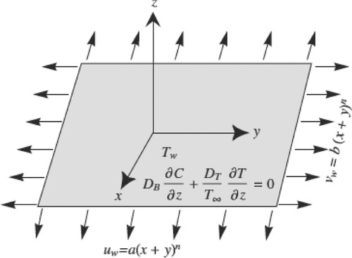
Consider an Eyring-Powell nanofluid 3D flow over a surface which is extended in a nonlinear manner in a Darcy-Forchheimer permeable medium with entropy generation analysis. The zero-mass flux and convective boundary conditions are taken at the surface with combined impacts of a chemical reaction and nonlinear radiative heat flux. The surface is stretched nonlinearly along x- and y-directions with velocities $\left[u_w=a{\left(x+y\right)}^n\right]$ and $\left[v_w=b{\left(x+y\right)}^n\right]$ respectively. However, the direction of the third axis (z-axis) is along the normal direction with $a,n,b>0.$ Figure 1 depicts the envisioned mathematical model.

Figure 1. Illustration of the envisaged model.

The Cauchy stress tensor T for the Eyring-Powel fluid is depicted as: (1) $\begin{array}{rl}\mathrm{T}& =-pI+\tau ,\end{array}$(1) (2) $\begin{array}{rl}{\rho }_f{a}_i& =-\mathrm{\nabla }p+\mathrm{\nabla }.\left({\tau }_{ij}\right),\end{array}$(2) where ${\tau }_{ij}$ represents the extra stress tensor [60]: (3) ${\tau }_{ij}=\mu \frac{\mathrm{\partial }{u}_i}{\mathrm{\partial }{x}_j}+\frac{1}{\text{β}}{\sinh }^{-1}\left(\left(\frac{1}{d_1}\right)\frac{\mathrm{\partial }{u}_i}{\mathrm{\partial }{x}_j}\right),$(3) with (4) $\begin{array}{rl}& {\sinh }^{-1}\left(\left(\frac{1}{d_1}\right)\frac{\mathrm{\partial }{u}_i}{\mathrm{\partial }{x}_j}\right)\cong \frac{1}{d_1}\frac{\mathrm{\partial }{u}_i}{\mathrm{\partial }{x}_j}-\frac{1}{6}{\left(\left(\frac{1}{d_1}\right)\frac{\mathrm{\partial }{u}_i}{\mathrm{\partial }{x}_j}\right)}^3,\\ & \times \left|\frac{1}{d_1}\frac{\mathrm{\partial }{u}_i}{\mathrm{\partial }{x}_j}\right|\prec 1,\end{array}$(4) and using boundary layer concept; for Eyring-Powell nanofluid 3D flow, the governing 3D equations are written as: (5) $\begin{array}{rl}& u_x+v_y+w_z=0,\end{array}$(5) (6) $\begin{array}{rl}& u{u}_x+v{u}_y+w{u}_z=\left(\nu +\frac{1}{{\rho }_f\text{β}{d}_1}\right)\\ & u_{zz}-\frac{1}{2\text{β}{d_1}^3{\rho }_f}(u_z{)}^2{u}_{zz}-\frac{\nu }{k^{\ast }}u-F{u}^2,\end{array}$(6) (7) $\begin{array}{rl}& u{v}_x+v{v}_y+w{v}_z=\left(\nu +\frac{1}{{\rho }_f\text{β}{d}_1}\right)v_{zz}\\ & -\frac{1}{2\text{β}{d_1}^3{\rho }_f}(v_z{)}^2{v}_{zz}-\frac{\nu }{k^{\ast }}v-F{v}^2,\end{array}$(7) (8) $\begin{array}{rl}& u{T}_x+v{T}_y+w{T}_z={\alpha }^{\ast }{T}_{zz}\\ & +\frac{{\left(\rho c\right)}_p}{{\left(\rho c\right)}_f}\left[D_B\left(T_z{C}_z\right)+\frac{D_T}{T_{\mathrm{\infty }}}{\left(T_z\right)}^2\right]-\frac{1}{{\left(\rho c\right)}_f}(q_r{)}_z,\end{array}$(8) (9) $\begin{array}{rl}& u{C}_x+v{C}_y+w{C}_z=D_B\left(C_{zz}\right)+\frac{D_T}{T_{\mathrm{\infty }}}\left(T_{zz}\right)-k_c\left(C-C_{\mathrm{\infty }}\right),\end{array}$(9) with associated boundary conditions:

At $z=0,$ $u=u_w,w=0,v=v_{w,}-k{T}_z=h_f\left(T_f-T\right),$ $D_B{C}_z+\left(\frac{D_T}{T_{\mathrm{\infty }}}\right)T_z=0,$

• when $z\to \mathrm{\infty }$. $u\to 0,$ $v\to 0,$ $T\to T_{\mathrm{\infty }},$ $C\to C_{\mathrm{\infty }}$. (10)

Here, (11) $F=\frac{C_b}{\left(x+y\right)k^{{\ast }^{1/2}}},{\alpha }^{\ast }=\frac{k}{{\left(\rho c\right)}_f},h_f=h(x+y{)}^{\frac{n-1}{2}}.$(11)

Using the following transformations: (12) $\begin{array}{rl}u& =\left[a{\left(x+y\right)}^n\right]f^{\mathrm{\prime }}\left(\zeta \right),v=\left[a{\left(x+y\right)}^n\right]g^{\mathrm{\prime }}\left(\zeta \right),\\ w& =-{\left(\frac{a\nu \left(n+1\right)}{2}\right)}^{1/2}(x+y{)}^{\left(n-1\right)/2}\\ & \left(\frac{n-1}{n+1}\zeta \left(f^{\mathrm{\prime }}+g^{\mathrm{\prime }}\right)+\left(f+g\right)\right),\\ \theta \left(\zeta \right)& =\frac{T-T_{\mathrm{\infty }}}{T_f-T_{\mathrm{\infty }}},\zeta =\sqrt{\left(\frac{a\left(n+1\right)}{2\nu }\right)}(x+y{)}^{\left(n-1\right)/2}z,\\ \phi \left(\zeta \right)& =\frac{C-C_{\mathrm{\infty }}}{C_{\mathrm{\infty }}}.\end{array}$(12)

The continuity Equation (5) is satisfied (i.e. mass is conserved), while Equations (6)–(10) take the form: (13) $\begin{array}{rl}& \left(1+\epsilon \right)f^{\mathrm{\prime }\mathrm{\prime }\mathrm{\prime }}-\left(\frac{2}{n+1}\right)Fr(f^{\mathrm{\prime }}{)}^2-\frac{\left(n+1\right)}{2}\epsilon \delta f^{\mathrm{\prime }\mathrm{\prime }2}{f}^{\mathrm{\prime }\mathrm{\prime }\mathrm{\prime }}\\ & +\left(f+g\right)f^{\mathrm{\prime }\mathrm{\prime }}-\left(\frac{2}{n+1}\right)\lambda f^{\mathrm{\prime }}\\ & -\left(\frac{2n}{n+1}\right)\left(f^{\mathrm{\prime }}+g^{\mathrm{\prime }}\right)f^{\mathrm{\prime }}=0,\end{array}$(13) (14) $\begin{array}{rl}& \left(1+\epsilon \right)g^{\mathrm{\prime }\mathrm{\prime }\mathrm{\prime }}-\left(\frac{2}{n+1}\right)Fr(g^{\mathrm{\prime }}{)}^2-\frac{\left(n+1\right)}{2}\epsilon \delta g^{\mathrm{\prime }\mathrm{\prime }2}{g}^{\mathrm{\prime }\mathrm{\prime }\mathrm{\prime }}\\ & +\left(f+g\right)g^{\mathrm{\prime }\mathrm{\prime }}-\left(\frac{2}{n+1}\right)\lambda g^{\mathrm{\prime }}\\ & -\left(\frac{2n}{n+1}\right)\left(f^{\mathrm{\prime }}+g^{\mathrm{\prime }}\right)g^{\mathrm{\prime }}=0,\end{array}$(14) (15) $\begin{array}{rl}& \left[1+Rd\frac{4}{3}{\left(1+\left({\theta }_f-1\right)\theta \right)}^3\right]{\theta }^{\mathrm{\prime }\mathrm{\prime }}+PrNb{\theta }^{\mathrm{\prime }}{\phi }^{\mathrm{\prime }}\\ & +\left[PrNt+4Rd{\left(1+\left({\theta }_f-1\right)\theta \right)}^2\left({\theta }_f-1\right)\right]{\theta }^{\mathrm{\prime }2}\\ & +Pr{\theta }^{\mathrm{\prime }}\left(f+g\right)=0,\end{array}$(15) (16) ${\phi }^{\mathrm{\prime }\mathrm{\prime }}+\frac{Nt}{Nb}{\theta }^{\mathrm{\prime }\mathrm{\prime }}+Scf{\phi }^{\mathrm{\prime }}+Scg{\phi }^{\mathrm{\prime }}-2\frac{Sc{\delta }_1}{n+1}\phi =0,$(16) with (17) $\begin{array}{l}f\left(0\right)=0,g\left(0\right)=0,f^{\mathrm{\prime }}\left(0\right)=1,g^{\mathrm{\prime }}\left(0\right)=\alpha ,{\theta }^{\mathrm{\prime }}\left(0\right)=\\ -\gamma \left[1-\theta \left(0\right)\right],Nb{\phi }^{\mathrm{\prime }}\left(0\right)+Nt{\theta }^{\mathrm{\prime }}\left(0\right)=0,\\ f^{\mathrm{\prime }}\left(\mathrm{\infty }\right)\to 0,g^{\mathrm{\prime }}\left(\mathrm{\infty }\right)\to 0,\theta \left(\mathrm{\infty }\right)\to 0,\phi \left(\mathrm{\infty }\right)\to 0.\end{array}$(17)

Distinct parameters defined above are given by: (18) $\begin{array}{l}\epsilon =\frac{1}{{\rho }_f\nu \text{β}{d}_1},\delta =\frac{a^3{\left(x+y\right)}^{3n-1}}{2\nu {d_1}^2},\lambda =\frac{\nu }{a{k}^{\ast }}(x+y{)}^{1-n},\\ Fr=\frac{C_b}{k^{{\ast }^{1/2}}},Rd=\frac{4{\sigma }^{\ast }{T_{\mathrm{\infty }}}^3}{k{k}^{\ast }},{\theta }_f=\frac{T_f}{T_{\mathrm{\infty }}},\\ \alpha =\frac{b}{a},Pr=\frac{\nu }{{\alpha }^{\ast }},\gamma =\frac{h}{k}\sqrt{\frac{2\nu }{a\left(n+1\right)}},Nt=\frac{{\left(\rho c\right)}_p{D}_T\left(T_f-T_{\mathrm{\infty }}\right)}{{\left(\rho c\right)}_f\nu T_{\mathrm{\infty }}},\\ Sc=\frac{\nu }{D_B},Nb=\frac{{\left(\rho c\right)}_p{D}_B{C}_{\mathrm{\infty }}}{{\left(\rho c\right)}_f\nu },{\delta }_1=\frac{k_c}{a}(x+y{)}^{1-n}.\end{array}$(18)

The local Nusselt number $\left(N{u}_x\right)$ is formulated as: (19) $N{u}_x=\frac{(x+y)q_r}{k(T_f-T_{\mathrm{\infty }})}.$(19)

Through the transformations defined in Equation (12), the local Nusselt number in nondimensional form is appended below: (20) $\begin{array}{rl}& N{u}_{x}R{e_x}^{-1/2}\\ & =-\sqrt{\left(\frac{n+1}{2}\right)}\left[\left(1+Rd{\left\{\left({\theta }_f-1\right)\theta \left(0\right)+1\right\}}^3\right)\right]{\theta }^{\mathrm{\prime }}\left(0\right),\end{array}$(20) whence $R{e}_x=\frac{u_w\left(x+y\right)}{\nu },$ characterizes local Reynolds number.

3. Solution by HAM

In 1992, Liao [49] anticipated the Homotopy analysis method. This technique is used for the formation of a series solution for a system of highly non-linear equations. Suitable preliminary estimates with related linear operators are defined as: (21) $\begin{array}{rl}{f}_0\left(\zeta \right)& =1-e^{-\zeta },g_0\left(\zeta \right)=\alpha \left(1-e^{-\zeta }\right),{\theta }_0\left(\zeta \right)\\ & =\frac{\gamma }{1+\gamma }{e}^{-\zeta },{\phi }_0\left(\zeta \right)=-\frac{\gamma }{1+\gamma }\frac{Nt}{Nb}{e}^{-\zeta },\end{array}$(21) (22) $L_f+f^{\mathrm{\prime }\mathrm{\prime }\mathrm{\prime }}-f^{\mathrm{\prime }},L_g=g^{\mathrm{\prime }\mathrm{\prime }\mathrm{\prime }}-g^{\mathrm{\prime }},L_{\theta }={\theta }^{\mathrm{\prime }\mathrm{\prime }}-\theta ,L_{\phi }={\phi }^{\mathrm{\prime }\mathrm{\prime }}-\phi .$(22) The aforementioned linear operators abide by the following characteristics: (21) $\begin{array}{rl}& L_f\{B_1+B_2{e}^{\zeta }+B_3{e}^{-\zeta }\}=0,\\ & L_g\{B_4+B_5{e}^{\zeta }+B_6{e}^{-\zeta }\}=0,\\ & L_{\theta }\{B_7{e}^{\zeta }+B_8{e}^{-\zeta }\}=0,L_{\theta }\{B_9{e}^{\zeta }+B_{10}{e}^{-\zeta }\}=0,\end{array}$(21) where $B_k\left(k=1\text{to}10\right),$ characterize the arbitrary constants.

4. Convergence analysis

The auxiliary parameters ${\hslash }_f,{\hslash }_g,{\hslash }_{\theta }and{\hslash }_{\phi }$ play a decisive role to determine the convergence of the Homotopy series solutions. The -curves are given in Figure 2. The permissible ranges of parameters are $-1.3\le {\hslash }_f\le -0.4,-1.4\le {\hslash }_g\le -0.3,-1.5\le {\hslash }_{\theta }\le -0.5,-1.4\le {\hslash }_{\phi }\le -0.4$. Table 1 is formed to see that the 25th approximation is enough for convergence purposes. It is comprehended that both graphical and numeric results are in total alignment.

Figure 2.  curves for $f,g,\theta ,\phi$.

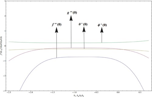
Table 1. The numeric formulation of the convergence for varied order of estimations with $\epsilon =0.3,\delta =0.1,Fr=0.1,n=0.3,Rd=0.4,Pr=1.0,Sc=1.0,Nt=0.1,\lambda =0.1,{\theta }_f=0.1,{\delta }_1=0.1,Nb=0.3,\gamma =\mathrm{0.3.}$

Order of approximations	$-{\mathit{f}}^{\mathrm{\prime }\mathrm{\prime }}\left(0\right)$	$-{\mathit{g}}^{\mathrm{\prime }\mathrm{\prime }}\left(0\right)$	$-{\mathit{\theta }}^{\mathrm{\prime }}\left(0\right)$	${\phi }^{\mathrm{\prime }}\left(0\right)$
1	0.72256	0.17195	0.20402	0.171341
10	0.73190	0.18697	0.20410	0.187403
15	0.74358	0.18700	0.20417	0.192546
20	0.75593	0.18739	0.20445	0.198149
25	0.77590	0.18840	0.20447	0.199150
30	0.77590	0.18840	0.20447	0.199150

5. Entropy generation analysis

The entropy volumetric equation for the Powell Eyring nanofluid flow is depicted by:

(24) $\begin{array}{rl}{S}_{gen}^{\mathrm{\prime }\mathrm{\prime }\mathrm{\prime }}& =\underset{HTI}{\underbrace{\frac{k}{{T_{\mathrm{\infty }}}^2}\left[{\left(\frac{\mathrm{\partial }T}{\mathrm{\partial }z}\right)}^2+\frac{16\sigma T^3}{3k{k}^{\ast }}{\left(\frac{\mathrm{\partial }T}{\mathrm{\partial }z}\right)}^2\right]}}\\ & +\underset{FFI}{\underbrace{\begin{array}{c}\frac{\mu }{T_{\mathrm{\infty }}}\left[\left(1+\frac{1}{\text{β}{\rho }_f{d}_1}\right){\left(\frac{\mathrm{\partial }u}{\mathrm{\partial }z}\right)}^2+\frac{1}{6\text{β}{\rho }_f{d_1}^3}{\left(\frac{\mathrm{\partial }u}{\mathrm{\partial }z}\right)}^4\right]+\frac{\mu }{T_{\mathrm{\infty }}}\\ \left[\left(1+\frac{1}{\text{β}{\rho }_f{d}_1}\right){\left(\frac{\mathrm{\partial }v}{\mathrm{\partial }z}\right)}^2+\frac{1}{6\text{β}{\rho }_f{d_1}^3}{\left(\frac{\mathrm{\partial }v}{\mathrm{\partial }z}\right)}^4\right]\end{array}}}\\ & +\underset{DI}{\underbrace{\left[\frac{RD}{C_{\mathrm{\infty }}}{\left(\frac{\mathrm{\partial }C}{\mathrm{\partial }z}\right)}^2+\frac{RD}{T_{\mathrm{\infty }}}\left(\frac{\mathrm{\partial }T}{\mathrm{\partial }z}\frac{\mathrm{\partial }C}{\mathrm{\partial }z}\right)\right]}},\end{array}$(24)

The Equation (24) contains the below-mentioned effects:

• Diffusive irreversibility (DI)

• Fluid friction irreversibility (FFI)

• Conduction effect or heat transfer irreversibility (HTI)

• And the entropy generation characteristic is expressed as: (25) $S_0^{\mathrm{\prime }\mathrm{\prime }\mathrm{\prime }}=\frac{{\left(\mathrm{\Delta }T\right)}^{2}k}{L^2{T}_{\mathrm{\infty }}^2}.$(25)

The entropy generation number $N_s$ is labelled by: $N_s=\frac{{S^{\mathrm{\prime }\mathrm{\prime }\mathrm{\prime }}}_{gen}}{{S^{\mathrm{\prime }\mathrm{\prime }\mathrm{\prime }}}_o}$ (26)

Employing Equation (12), the entropy generation is simplified as: (27) $\begin{array}{rl}{N}_s& =\frac{{S^{\mathrm{\prime }\mathrm{\prime }\mathrm{\prime }}}_{gen}}{{S^{\mathrm{\prime }\mathrm{\prime }\mathrm{\prime }}}_0}=\left[\frac{a{\left(x+y\right)}^n{L}^2}{2\nu }\right]{\theta }^{\mathrm{\prime }2}\\ & +\left[\frac{16\sigma T_{\mathrm{\infty }}^{3}a{L}^2{\left(x+y\right)}^n}{6\nu k{k}^{\ast }}\right]{\theta }^{\mathrm{\prime }2}\\ & +\left[\frac{a^3{L}^2{T}_{\mathrm{\infty }}\mu {\left(x+y\right)}^{3n}\left(1+\epsilon \right)}{2\nu k{\left(\Delta T\right)}^2}\right]\left({\left(f^{\mathrm{\prime }\mathrm{\prime }}\right)}^2+{\left(g^{\mathrm{\prime }\mathrm{\prime }}\right)}^2\right)\\ & -\left[\frac{a^6{L}^2{T}_{\mathrm{\infty }}\mu \epsilon {\left(x+y\right)}^{6n-1}}{24k{\left(\Delta T\right)}^2{\nu }^2}\right]\left({\left(f^{\mathrm{\prime }\mathrm{\prime }}\right)}^4+{\left(g^{\mathrm{\prime }\mathrm{\prime }}\right)}^4\right)\\ & +\left[\frac{a{\left(x+y\right)}^{n}RD{T}_{\mathrm{\infty }}{L}^2\left(\Delta C\right)}{2\nu k\left(\Delta T\right)}\right]{\theta }^{\mathrm{\prime }}{\phi }^{\mathrm{\prime }}\\ & +\left[\frac{a{\left(x+y\right)}^n{T}_{\mathrm{\infty }}^2{L}^{2}RD{\left(\Delta C\right)}^2}{2\nu k{\left(\Delta T\right)}^2}\right]{{\phi }^{\mathrm{\prime }}}^2,\end{array}$(27)

Finally, the entropy number in nondimensional form is stated as: (28) $\begin{array}{rl}{N}_S& =\frac{{S^{\mathrm{\prime }\mathrm{\prime }\mathrm{\prime }}}_{gen}}{{S^{\mathrm{\prime }\mathrm{\prime }\mathrm{\prime }}}_0}=\frac{Re}{2}\left(1+\frac{4}{3}Rd\right){{\theta }^{\mathrm{\prime }}}^2\left(\zeta \right)+\frac{Re{\lambda }_1}{2}{\left(\frac{\chi }{\Omega }\right)}^2{\phi }^{\mathrm{\prime }2}\\ & +\frac{Re{\lambda }_1}{2}\left(\frac{\chi }{\Omega }\right){\theta }^{\mathrm{\prime }}{\phi }^{\mathrm{\prime }}\\ & +\left(\left(1+\epsilon \right)\left({\left(f^{\mathrm{\prime }\mathrm{\prime }}\right)}^2+{\left(g^{\mathrm{\prime }\mathrm{\prime }}\right)}^2\right)-\frac{\epsilon \delta }{6}\left({\left(f^{\mathrm{\prime }\mathrm{\prime }}\right)}^4+{\left(g^{\mathrm{\prime }\mathrm{\prime }}\right)}^4\right)\right)\\ & \times \left(\frac{Br.Re}{2\Omega }\right),\end{array}$(28) where (29) $Re=\frac{u_w{L}^2}{\nu },Br=\frac{\mu {u_w}^2}{k\Delta T},\Omega =\frac{\Delta T}{T_{\mathrm{\infty }}},\chi =\frac{\Delta C}{C_{\mathrm{\infty }}},{\lambda }_1=\frac{RD{C}_{\mathrm{\infty }}}{k}.$(29)

6. Results and discussion

This section is designated to observe the influence of several parameters on associated distributions. Figures 3 and 4 are outlined to see the outcome of fluid parameters $\epsilon$ and $\delta$ on the velocity profile. It is understood that the velocity profile is an escalating and diminishing function for $\epsilon$ and $\delta$ respectively. Since $\epsilon =\frac{1}{{\rho }_f\nu \text{β}{d}_1},$ so by increasing $\epsilon ,$ liquid viscosity $\left({\rho }_f\nu \text{β}{d}_1\right)$ reduces, which ultimately enhances the velocity. (When $\epsilon$ increases, fluid exhibit the shear-thinning property which increases velocity). Whereas, by increasing $\delta$, velocity reduces, This is because the viscosity of the liquid enhances by escalating values of $\delta$. Illustration of Forchheimer number $Fr$ on the fluid velocity is displayed in Figure 5. It is perceived from the figure that the velocity is decreased for $Fr.$ For higher values of $Fr,$ permeability increases which leads to resistance in a fluid flow. Thus, lowering the fluid velocity. To understand the consequences of the Radiation parameter $Rd$ on the temperature distribution Figure 6 is sketched. It is visualized that the temperature of the liquid augments versus large values of $Rd$. Larger estimates of $Rd$ obviously increase the temperature of the nanofluid as it is in direct proportionate to the nanofluid temperature at infinity. Figures 7 and 8 are drawn to establish the effect of the chemical reaction parameter ${\delta }_1$, for the destructive ${\delta }_1>0$ case, and generative ${\delta }_1<0$ case, respectively on the concentration field. An opposing trend in both cases is witnessed for the concentration profile. A slight decrement in the boundary layer thickness can be observed in case of ${\delta }_1>0$ for mounting values of ${\delta }_1$. Escalating estimates of ${\delta }_1$ suppresses the concentration of the liquid. Also, large values of ${\delta }_1$ would result in less diffusion, thus leading to a reduction in diffusion. To visualize the influence of the Biot number $\gamma$ versus temperature profile, Figure 9 is drawn. As $\gamma$ is linked with the heat transfer at the boundary. Thus, upsurge in $\gamma$, augments the thermal boundary layer, and ultimately enhanced temperature is perceived. The impacts of and the Brinkman number Br and the Reynold number $Re$ on the entropy generation number $Ns$ are portrayed in Figures 10 and 11 respectively. The large estimates of both parameters play a vital role in the generation of entropy owing to their resistive role. Thus, creating chaos in the fluid flow. Figure 12 is drawn to witness the consequences of Schmidt number$Sc$versus the concentration field. For higher estimates of $Sc$ feeble concentration is observed. As the Schmidt number is inverse proportionate to mass diffusivity. Thus, large values of $Sc$ result in lowering mass diffusivity that allows shallower penetration (infusion) of the solutal effect. Consequently, this feeble mass diffusivity lowers the concentration. The characteristics of ${\delta }_1$ and $Nt$ on the Nusselt number are shown in Figure 13. Interestingly Nusselt number decreases for both $Nt$ and ${\delta }_1$. Table 2 is erected to give a comparison with Ariel [50] in limiting the case. A remarkable consensus is obtained in this regard.

Figure 3. Upshot of $\epsilon$ versus $f^{\mathrm{\prime }}$

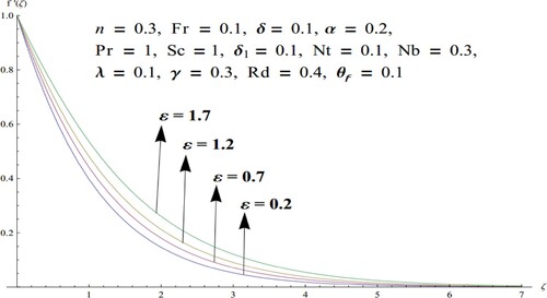
Figure 4. Upshot of $\delta$ versus $f^{\mathrm{\prime }}$

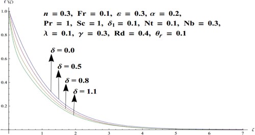
Figure 5. Upshot of $Fr$ versus $f^{\mathrm{\prime }}$

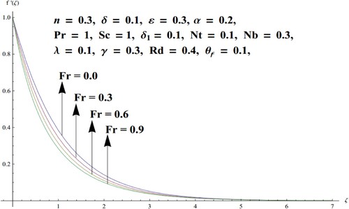
Figure 6. Upshot of Rd versus $\theta$.

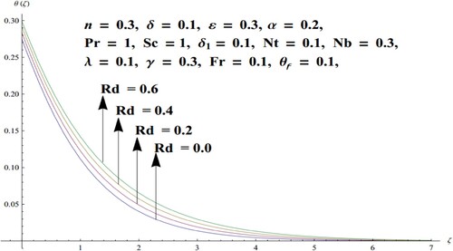
Figure 7. Upshot of ${\delta }_1>0$ versus $\phi$.

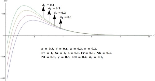
Figure 8. Upshot of ${\delta }_1<0$ versus $\phi$.

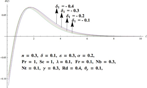
Figure 9. Upshot of $\gamma$ versus $\theta$.

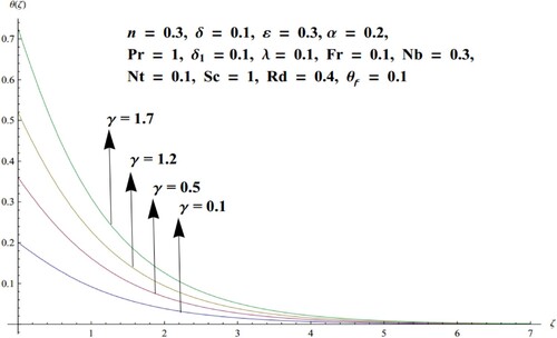
Figure 10. Upshot of Br versus $Ns$_.

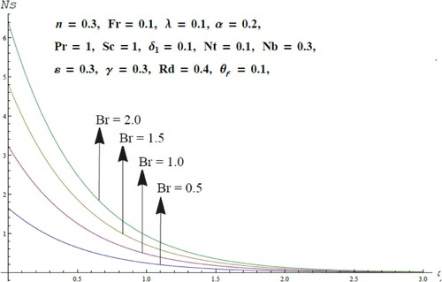
Figure 11. Upshot of $Re$ versus $Ns$_.

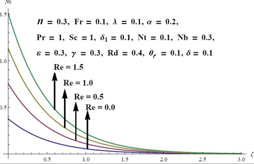
Figure 12. Upshot of $Sc$ versus $\phi$.

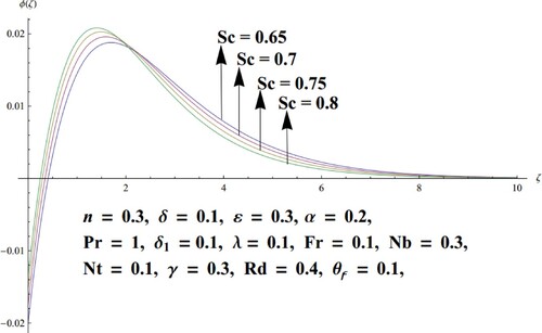
Figure 13. Illustration of $N{u}_{x}R{e}_x^{-1/2}$ versus ${\delta }_1$ and Nt.

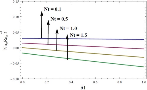
Table 2. Comparative statement of $-f^{\mathrm{\prime }\mathrm{\prime }}\left(0\right)$ with Ariel [50] for the numerous estimates of $\alpha$.

		$-f^{\mathrm{\prime }\mathrm{\prime }}\left(0\right)$
$\alpha$	HPM	Exact	Present
0	1	1	1
0.1	1.017027	1.020260	1.020261
0.2	1.034587	1.039495	1.039496
0.3	1.052470	1.057955	1.057955
0.4	1.070529	1.075788	1.075788
0.5	1.088662	1.093095	1.093096
0.6	1.106797	1.109947	1.109947
0.7	1.124882	1.126398	1.126399
0.8	1.142879	1.142489	1.142489
0.9	1.60762	1.158254	1.158255
1.0	1.178511	1.173721	1.173722

7. Concluding remarks

The present consideration is to analyse the steady 3D Eyring Powell nanofluid flow past a nonlinear Darcy-Forchheimer spongy stretchable surface with entropy generation analysis. Originality of the presented model is improved by the inclusion of the radiative heat flux with zero mass flux condition at the surface. Analytical results in the form of series solution are obtained for the given problem via HAM. The major outcomes of the problem are:

• It is noticed that in the existence of Darcy-Forchheimer number, the liquid velocity reduces.

• For higher estimates of Schmidt number feeble concentration is observed.

• Fluid temperature augments versus larger values of the Radiation parameter.

• Entropy is strengthened for large estimates of Brinkman and Reynolds numbers.

• Large Biot number estimates augment the fluid temperature.

Acknowledgement

This research was supported by Korea Institute for Advancement of Technology (KIAT) grant funded by the Korea Government (MOTIE) (P0012724, The Competency Development Program for Industry Specialist) and the Soonchunhyang University Research Fund.

Disclosure statement

No potential conflict of interest was reported by the author(s).

Appendix:

Solving Equation (6) by transformations (12) to get Equation (12) as follows: (6) $\begin{array}{rl}u{u}_x+v{u}_y+w{u}_z& =\left(\nu +\frac{1}{{\rho }_f\text{β}{d}_1}\right)u_{zz}-\frac{1}{2\text{β}{d_1}^3{\rho }_f}(u_z{)}^2{u}_{zz}\\ & -\frac{\nu }{k^{\ast }}u-F{u}^2,\end{array}$(6) where (6a) $\begin{array}{rl}u& =\left[a{\left(x+y\right)}^n\right]f^{\mathrm{\prime }}\left(\zeta \right),v=\left[a{\left(x+y\right)}^n\right]g^{\mathrm{\prime }}\left(\zeta \right),\\ w& =-{\left(\frac{a\nu \left(n+1\right)}{2}\right)}^{1/2}(x+y{)}^{\left(n-1\right)/2}\\ & \times \left(\frac{n-1}{n+1}\zeta \left(f^{\mathrm{\prime }}+g^{\mathrm{\prime }}\right)+\left(f+g\right)\right),\\ u_x& =a(x+y{)}^{n-1}\left[n{f}^{\mathrm{\prime }}+\frac{\left(n-1\right)}{2}\zeta f^{\mathrm{\prime }\mathrm{\prime }}\left(\zeta \right)\right],\\ u_y& =a(x+y{)}^{n-1}\left[n{f}^{\mathrm{\prime }}+\frac{\left(n-1\right)}{2}\zeta f^{\mathrm{\prime }\mathrm{\prime }}\left(\zeta \right)\right],\\ u_z& =\left[a^{\frac{3}{2}}{\left(x+y\right)}^{\frac{\left(3n-1\right)}{2}}\sqrt{\frac{\left(n+1\right)}{2\nu }}\right]f^{\mathrm{\prime }\mathrm{\prime }}\left(\zeta \right),\\ u_{zz}& =\left[a^2{\left(x+y\right)}^{2n-1}\frac{\left(n+1\right)}{2\nu }\right]f^{\mathrm{\prime }\mathrm{\prime }\mathrm{\prime }}\left(\zeta \right),\end{array}$(6a)

Putting Equation (6a) in Equation (6), we get (6b) $\begin{array}{rl}& a(x+y{)}^n{f}^{\mathrm{\prime }}\left[a{\left(x+y\right)}^{n-1}\left(n{f}^{\mathrm{\prime }}+\frac{\left(n-1\right)}{2}\zeta f^{\mathrm{\prime }\mathrm{\prime }}\right)\right]\\ & +a(x+y{)}^n{g}^{\mathrm{\prime }}\left[a{\left(x+y\right)}^{n-1}\left(n{f}^{\mathrm{\prime }}+\frac{\left(n-1\right)}{2}\zeta f^{\mathrm{\prime }\mathrm{\prime }}\right)\right]\\ & -{\left(\frac{a\nu \left(n+1\right)}{2}\right)}^{1/2}(x+y{)}^{\left(n-1\right)/2}\left(\frac{n-1}{n+1}\zeta \left(f^{\mathrm{\prime }}+g^{\mathrm{\prime }}\right)+\left(f+g\right)\right)\\ & \times \left[a^{\frac{3}{2}}{\left(x+y\right)}^{\frac{\left(3n-1\right)}{2}}\sqrt{\frac{\left(n+1\right)}{2\nu }}{f}^{\mathrm{\prime }\mathrm{\prime }}\right]\\ & =\left(\nu +\frac{1}{{\rho }_f\text{β}{d}_1}\right)\left[a^2{\left(x+y\right)}^{2n-1}\frac{\left(n+1\right)}{2\nu }{f}^{\mathrm{\prime }\mathrm{\prime }\mathrm{\prime }}\right]\\ & -\frac{1}{2\text{β}{d_1}^3{\rho }_f}{\left(a^{\frac{3}{2}}{\left(x+y\right)}^{\frac{\left(3n-1\right)}{2}}\sqrt{\frac{\left(n+1\right)}{2\nu }}{f}^{\mathrm{\prime }\mathrm{\prime }}\right)}^2\\ & \left[a^2{\left(x+y\right)}^{2n-1}\frac{\left(n+1\right)}{2\nu }{f}^{\mathrm{\prime }\mathrm{\prime }\mathrm{\prime }}\right]\\ & -\frac{\nu }{k^{\ast }}\left(a{\left(x+y\right)}^n{f}^{\mathrm{\prime }}\right)-F(a{\left(x+y\right)}^n{f}^{\mathrm{\prime }}{)}^2,\end{array}$(6b)

After simplification of brackets, Equation (6b) can be written as: (6c) $\begin{array}{rl}& a^2(x+y{)}^{2n-1}n(f^{\mathrm{\prime }}{)}^2+a^2(x+y{)}^{2n-1}\frac{\left(n-1\right)}{2}\zeta f^{\mathrm{\prime }}{f}^{\mathrm{\prime }\mathrm{\prime }}\\ & +a^2(x+y{)}^{2n-1}n{g}^{\mathrm{\prime }}{f}^{\mathrm{\prime }}+a^2(x+y{)}^{2n-1}\frac{\left(n-1\right)}{2}\zeta g^{\mathrm{\prime }}{f}^{\mathrm{\prime }\mathrm{\prime }}\\ & -a^2(x+y{)}^{2n-1}\frac{\left(n+1\right)}{2}\left(f+g\right)f^{\mathrm{\prime }\mathrm{\prime }}\\ & -a^2(x+y{)}^{2n-1}\frac{\left(n-1\right)}{2}\zeta \left(f^{\mathrm{\prime }}+g^{\mathrm{\prime }}\right)f^{\mathrm{\prime }\mathrm{\prime }}\\ & =\left(\nu +\frac{1}{{\rho }_f\text{β}{d}_1}\right)a^2(x+y{)}^{2n-1}\frac{\left(n+1\right)}{2\nu }{f}^{\mathrm{\prime }\mathrm{\prime }\mathrm{\prime }}\\ & -\frac{a^5{\left(x+y\right)}^{5n-2}}{2{\rho }_f\text{β}{d}_1^3}{\left(\frac{n+1}{2\nu }\right)}^2(f^{\mathrm{\prime }\mathrm{\prime }}{)}^2{f}^{\mathrm{\prime }\mathrm{\prime }\mathrm{\prime }}\\ & -\frac{a\nu {\left(x+y\right)}^n}{k^{\ast }}{f}^{\mathrm{\prime }}-F{a}^2(x+y{)}^{2n}(f^{\mathrm{\prime }}{)}^2,\end{array}$(6c)

Take, $\left(\frac{a^2\left(n+1\right){\left(x+y\right)}^{2n-1}}{2}\right)$ common from both sides of equation and from L.H.S add 2nd and 4th term and cancel it by 6th term and further take $f^{\mathrm{\prime }}$ common from 1st and 3rd terms, we get equation (6d) as follows: (6d) $\begin{array}{rl}& \frac{2n}{n+1}\left(f^{\mathrm{\prime }}+g^{\mathrm{\prime }}\right)f^{\mathrm{\prime }}-\left(f+g\right)f^{\mathrm{\prime }\mathrm{\prime }}=\left(\nu +\frac{1}{{\rho }_f\text{β}{d}_1}\right)\frac{f^{\mathrm{\prime }\mathrm{\prime }\mathrm{\prime }}}{\nu }-\\ & \frac{a^3{\left(x+y\right)}^{3n-1}\left(n+1\right)}{4{\nu }^2{\rho }_f\text{β}{d}_1^3}(f^{\mathrm{\prime }\mathrm{\prime }}{)}^2{f}^{\mathrm{\prime }\mathrm{\prime }\mathrm{\prime }}-\frac{2\nu {\left(x+y\right)}^{1-n}}{a\left(n+1\right)k^{\ast }}{f}^{\mathrm{\prime }}\\ & -\frac{2F}{\left(x+y\right)\left(n+1\right)}(f^{\mathrm{\prime }}{)}^2,\end{array}$(6d)

After incorporating the dimensionless parameters (18) into Equation (6d), we get a revised subsequent equation: $\begin{array}{rl}& \left(1+\epsilon \right)f^{\mathrm{\prime }\mathrm{\prime }\mathrm{\prime }}-\left(\frac{2}{n+1}\right)Fr(f^{\mathrm{\prime }}{)}^2-\frac{\left(n+1\right)}{2}\epsilon \delta f^{\mathrm{\prime }\mathrm{\prime }2}{f}^{\mathrm{\prime }\mathrm{\prime }\mathrm{\prime }}+\left(f+g\right)f^{\mathrm{\prime }\mathrm{\prime }}\\ & -\left(\frac{2}{n+1}\right)\lambda f^{\mathrm{\prime }}\\ & -\left(\frac{2n}{n+1}\right)\left(f^{\mathrm{\prime }}+g^{\mathrm{\prime }}\right)f^{\mathrm{\prime }}=0,\end{array}$This is the Equation (12) of the mathematical modelling.

Similar procedure would be followed for the Equation (7) to get Equation (14), as it was used for the above Equation (12) we get, $\begin{array}{rl}& \left(1+\epsilon \right)g^{\mathrm{\prime }\mathrm{\prime }\mathrm{\prime }}-\left(\frac{2}{n+1}\right)Fr(g^{\mathrm{\prime }}{)}^2-\frac{\left(n+1\right)}{2}\epsilon \delta g^{\mathrm{\prime }\mathrm{\prime }2}{g}^{\mathrm{\prime }\mathrm{\prime }\mathrm{\prime }}\\ & +\left(f+g\right)g^{\mathrm{\prime }\mathrm{\prime }}-\left(\frac{2}{n+1}\right)\lambda g^{\mathrm{\prime }}\\ & -\left(\frac{2n}{n+1}\right)\left(f^{\mathrm{\prime }}+g^{\mathrm{\prime }}\right)g^{\mathrm{\prime }}=0,\end{array}$This is the Equation (14) of the mathematical modelling.

Solving Equation (8) (8) $\begin{array}{rl}u{T}_x+v{T}_y+w{T}_z& ={\alpha }^{\ast }{T}_{zz}+\frac{{\left(\rho c\right)}_p}{{\left(\rho c\right)}_f}\left[D_B\left(T_z{C}_z\right)+\frac{D_T}{T_{\mathrm{\infty }}}{\left(T_z\right)}^2\right]\\ & -\frac{1}{{\left(\rho c\right)}_f}(q_r{)}_z,\end{array}$(8) with the help of (8a) $\begin{array}{rl}u& =\left[a{\left(x+y\right)}^n\right]f^{\mathrm{\prime }}\left(\zeta \right),v=\left[a{\left(x+y\right)}^n\right]g^{\mathrm{\prime }}\left(\zeta \right),\\ w& =-{\left(\frac{a\nu \left(n+1\right)}{2}\right)}^{1/2}(x+y{)}^{\left(n-1\right)/2}\\ & \times \left(\frac{n-1}{n+1}\zeta \left(f^{\mathrm{\prime }}+g^{\mathrm{\prime }}\right)+\left(f+g\right)\right),\\ T_x& =\left[\frac{\zeta \left(n-1\right)\left(T_f-T_{\mathrm{\infty }}\right)}{2\left(x+y\right)}\right]{\theta }^{\mathrm{\prime }}\left(\zeta \right),\\ T_y& =\left[\frac{\zeta \left(n-1\right)\left(T_f-T_{\mathrm{\infty }}\right)}{2\left(x+y\right)}\right]{\theta }^{\mathrm{\prime }}\left(\zeta \right),\\ T_z& =\left[\left(T_f-T_{\mathrm{\infty }}\right){\left(x+y\right)}^{\frac{\left(n-1\right)}{2}}\sqrt{\frac{a\left(n+1\right)}{2\nu }}\right]{\theta }^{\mathrm{\prime }}\left(\zeta \right),\\ C_z& =\left[C_{\mathrm{\infty }}{\left(x+y\right)}^{\left(n-1\right)/2}\sqrt{\frac{a\left(n+1\right)}{2\nu }}\right]{\phi }^{\mathrm{\prime }},\\ T_{zz}& =\left[\frac{a\left(n+1\right)}{2\nu }\left(T_f-T_{\mathrm{\infty }}\right){\left(x+y\right)}^{n-1}\right],q_r=-\frac{16{\sigma }^{\ast }}{3k^{\ast }}{T}^3\frac{\mathrm{\partial }T}{\mathrm{\partial }z},\\ \frac{\mathrm{\partial }{q}_r}{\mathrm{\partial }z}& =-\frac{16{\sigma }^{\ast }}{3k^{\ast }}\frac{\mathrm{\partial }}{\mathrm{\partial }z}\left[T^3\frac{\mathrm{\partial }T}{\mathrm{\partial }z}\right]=\frac{\mathrm{\partial }{T}^3}{\mathrm{\partial }z}\frac{\mathrm{\partial }T}{\mathrm{\partial }z}+T^3\frac{{\mathrm{\partial }}^{2}T}{\mathrm{\partial }{z}^2}\\ & =3T^2{\left(\frac{\mathrm{\partial }T}{\mathrm{\partial }z}\right)}^2+T^3\left(\frac{{\mathrm{\partial }}^{2}T}{\mathrm{\partial }{z}^2}\right),\end{array}$(8a) Putting Equation (8b) in Equation (8), we get (8b) $\begin{array}{rl}& a(x+y{)}^n{f}^{\mathrm{\prime }}\left[\frac{\left(n-1\right)\left(T_f-T_{\mathrm{\infty }}\right)\zeta }{2\left(x+y\right)}{\theta }^{\mathrm{\prime }}\right]\\ & +a(x+y{)}^n{g}^{\mathrm{\prime }}\left[\frac{\left(n-1\right)\left(T_f-T_{\mathrm{\infty }}\right)\zeta }{2\left(x+y\right)}{\theta }^{\mathrm{\prime }}\right]\\ & -{\left(\frac{a\nu \left(n+1\right)}{2}\right)}^{1/2}(x+y{)}^{\left(n-1\right)/2}\left(\frac{n-1}{n+1}\zeta \left(f^{\mathrm{\prime }}+g^{\mathrm{\prime }}\right)+\left(f+g\right)\right)\\ & \times \left[\left(T_f-T_{\mathrm{\infty }}\right){\left(x+y\right)}^{\left(n-1\right)/2}\sqrt{\frac{a\left(n+1\right)}{2\nu }}{\theta }^{\mathrm{\prime }}\right]\\ & ={\alpha }^{\ast }\left[\frac{a\left(n+1\right)\left(T_f-T_{\mathrm{\infty }}\right)}{2\nu }{\left(x+y\right)}^{n-1}{\theta }^{\mathrm{\prime }\mathrm{\prime }}\right]+\\ & \frac{{\left(\rho c\right)}_p}{{\left(\rho c\right)}_f}\left[D_B\left(\left(T_f-T_{\mathrm{\infty }}\right){\left(x+y\right)}^{\left(n-1\right)/2}\sqrt{\frac{a\left(n+1\right)}{2\nu }}{\theta }^{\mathrm{\prime }}\right)\right.\\ & \times \left({\left(x+y\right)}^{\left(n-1\right)/2}{C}_{\mathrm{\infty }}\sqrt{\frac{a\left(n+1\right)}{2\nu }}{\phi }^{\mathrm{\prime }}\right)+\frac{D_T}{T_{\mathrm{\infty }}}\\ & \left.\times {\left(\left(T_f-T_{\mathrm{\infty }}\right){\left(x+y\right)}^{\left(n-1\right)/2}\sqrt{\frac{a\left(n+1\right)}{2\nu }}{\theta }^{\mathrm{\prime }}\right)}^2\right]\\ & +\frac{16{\sigma }^{\ast }}{3k^{\ast }{\left(\rho c\right)}_f}\left[3{\left(T_{\mathrm{\infty }}+\theta \left(T_f-T_{\mathrm{\infty }}\right)\right)}^2\right.\\ & \times {\left({\theta }^{\mathrm{\prime }}\left(T_f-T_{\mathrm{\infty }}\right){\left(x+y\right)}^{\left(n-1\right)/2}\sqrt{\frac{a\left(n+1\right)}{2\nu }}\right)}^2\\ & +{\left(T_{\mathrm{\infty }}+\theta \left(T_f-T_{\mathrm{\infty }}\right)\right)}^3\\ & \left.\times \left(\frac{a\left(n+1\right)\left(T_f-T_{\mathrm{\infty }}\right)}{2\nu }{\left(x+y\right)}^{n-1}{\theta }^{\mathrm{\prime }\mathrm{\prime }}\right)\right]\end{array}$(8b)

After simplification of brackets, Equation (8b) is modified as: (8c) $\begin{array}{rl}& \left[\frac{a{\left(x+y\right)}^{n-1}\left(n-1\right)\left(T_f-T_{\mathrm{\infty }}\right)\zeta }{2}\right]f^{\mathrm{\prime }}{\theta }^{\mathrm{\prime }}\\ & +\left[\frac{a{\left(x+y\right)}^{n-1}\left(n-1\right)\left(T_f-T_{\mathrm{\infty }}\right)\zeta }{2}\right]g^{\mathrm{\prime }}{\theta }^{\mathrm{\prime }}\\ & -\left[\frac{a\left(n+1\right)\left(T_f-T_{\mathrm{\infty }}\right){\left(x+y\right)}^{n-1}}{2}\right]\left(f+g\right){\theta }^{\mathrm{\prime }}\\ & -\left[\frac{a\left(n-1\right)\left(T_f-T_{\mathrm{\infty }}\right){\left(x+y\right)}^{n-1}\zeta }{2}\right]\left(f^{\mathrm{\prime }}+g^{\mathrm{\prime }}\right){\theta }^{\mathrm{\prime }}\\ & ={\alpha }^{\ast }\left[\frac{a\left(n+1\right)\left(T_f-T_{\mathrm{\infty }}\right)}{2\nu }{\left(x+y\right)}^{n-1}{\theta }^{\mathrm{\prime }\mathrm{\prime }}\right]+\\ & \frac{{\left(\rho c\right)}_p}{{\left(\rho c\right)}_f}\left[\frac{a{D}_B{C}_{\mathrm{\infty }}\left(n+1\right){\left(x+y\right)}^{n-1}\left(T_f-T_{\mathrm{\infty }}\right)}{2\nu }{\phi }^{\mathrm{\prime }}{\theta }^{\mathrm{\prime }}\right.\\ & \left.+\frac{D_T}{T_{\mathrm{\infty }}}\left(\frac{a\left(n+1\right){\left(T_f-T_{\mathrm{\infty }}\right)}^2{\left(x+y\right)}^{n-1}}{2\nu }{\left({\theta }^{\mathrm{\prime }}\right)}^2\right)\right]\\ & +\frac{16{\sigma }^{\ast }}{k^{\ast }{\left(\rho c\right)}_f}\left[\left(\frac{a\left(n+1\right){\left(x+y\right)}^{n-1}{\left(T_f-T_{\mathrm{\infty }}\right)}^2}{2\nu }\right)\right.\\ & \left.{\left(T_{\mathrm{\infty }}+\theta \left(T_f-T_{\mathrm{\infty }}\right)\right)}^2{\left({\theta }^{\mathrm{\prime }}\right)}^2\right]\\ & \times \left[{\left(T_{\mathrm{\infty }}+\theta \left(T_f-T_{\mathrm{\infty }}\right)\right)}^3\right.\\ & \times \left.\left(\frac{a\left(n+1\right)\left(T_f-T_{\mathrm{\infty }}\right)}{2\nu }{\left(x+y\right)}^{n-1}{\theta }^{\mathrm{\prime }\mathrm{\prime }}\right)\right]\\ & +\frac{16{\sigma }^{\ast }}{3k^{\ast }{\left(\rho c\right)}_f}\left[\left(\frac{a\left(n+1\right){\left(x+y\right)}^{n-1}\left(T_f-T_{\mathrm{\infty }}\right)}{2\nu }\right)\right.\\ & \left.\times {\left(T_{\mathrm{\infty }}+\theta \left(T_f-T_{\mathrm{\infty }}\right)\right)}^3{\theta }^{\mathrm{\prime }\mathrm{\prime }}\right],\end{array}$(8c) Take, $\left(\frac{a{\alpha }^{\ast }\left(T_f-T_{\mathrm{\infty }}\right)\left(n+1\right){\left(x+y\right)}^{n-1}}{2\nu }\right)$ common from both sides of equation and from L.H.S add 1^st and 2nd term and cancel it by 4th term, we get equation (8d) as follows: (8d) $\begin{array}{rl}& -\frac{\nu }{{\alpha }^{\ast }}\left(f+g\right){\theta }^{\mathrm{\prime }}={\theta }^{\mathrm{\prime }\mathrm{\prime }}+\frac{{\left(\rho c\right)}_p}{{\left(\rho c\right)}_f}\left(\frac{D_B{C}_{\mathrm{\infty }}}{{\alpha }^{\ast }}{\phi }^{\mathrm{\prime }}{\theta }^{\mathrm{\prime }}\right)\\ & +\frac{{\left(\rho c\right)}_p}{{\left(\rho c\right)}_f}\left(\frac{D_T\left(T_f-T_{\mathrm{\infty }}\right)}{{\alpha }^{\ast }{T}_{\mathrm{\infty }}}{\left({\theta }^{\mathrm{\prime }}\right)}^2\right)\\ & \frac{{\left(\rho c\right)}_p}{{\left(\rho c\right)}_f}\left[\frac{a{D}_B{C}_{\mathrm{\infty }}\left(n+1\right)\left(T_f-T_{\mathrm{\infty }}\right)}{2\nu }{\phi }^{\mathrm{\prime }}{\theta }^{\mathrm{\prime }}\right.\\ & \left.+\frac{D_T}{T_{\mathrm{\infty }}}\left(\frac{a\left(n+1\right){\left(T_f-T_{\mathrm{\infty }}\right)}^2{\left(x+y\right)}^{n-1}}{2\nu }{\left({\theta }^{\mathrm{\prime }}\right)}^2\right)\right]\\ & +\frac{16{\sigma }^{\ast }}{{\alpha }^{\ast }{k}^{\ast }{\left(\rho c\right)}_f}\left[{\left(T_{\mathrm{\infty }}+\theta \left(T_f-T_{\mathrm{\infty }}\right)\right)}^2\left(T_f-T_{\mathrm{\infty }}\right){\left({\theta }^{\mathrm{\prime }}\right)}^2\right]\\ & +\frac{16{\sigma }^{\ast }}{3{\alpha }^{\ast }{k}^{\ast }{\left(\rho c\right)}_f}\left[{\left(T_{\mathrm{\infty }}+\theta \left(T_f-T_{\mathrm{\infty }}\right)\right)}^3{\theta }^{\mathrm{\prime }\mathrm{\prime }}\right],\end{array}$(8d)

Take $T_{\mathrm{\infty }}$ common from last two terms of Equation (8d), and simply some terms, we get, (8e) $\begin{array}{rl}& -\frac{\nu }{{\alpha }^{\ast }}\left(f+g\right){\theta }^{\mathrm{\prime }}={\theta }^{\mathrm{\prime }\mathrm{\prime }}+\frac{16{\sigma }^{\ast }{T}_{\mathrm{\infty }}^3}{3k{k}^{\ast }}\\ & \times {\left(1+\left(\frac{T_f}{T_{\mathrm{\infty }}}-1\right)\theta \right)}^3+\frac{{\left(\rho c\right)}_p{D}_B{C}_{\mathrm{\infty }}}{{\alpha }^{\ast }{\left(\rho c\right)}_f}{\theta }^{\mathrm{\prime }}{\phi }^{\mathrm{\prime }}\\ & +\frac{{\left(\rho c\right)}_p{D}_T\left(T_f-T_{\mathrm{\infty }}\right)}{{\alpha }^{\ast }{\left(\rho c\right)}_f{T}_{\mathrm{\infty }}}({\theta }^{\mathrm{\prime }}{)}^2+\frac{16{\sigma }^{\ast }{T}_{\mathrm{\infty }}^3}{k{k}^{\ast }}\\ & \times \left({\left(1+\left(\frac{T_f}{T_{\mathrm{\infty }}}-1\right)\theta \right)}^2\left(\frac{T_f}{T_{\mathrm{\infty }}}-1\right)\right)({\theta }^{\mathrm{\prime }}{)}^2,\end{array}$(8e)

After incorporating the dimensionless parameters (18) into Equation (8e), we get a revised equation that is as following: $\begin{array}{rl}& \left(1+Rd\frac{4}{3}{\left(1+\left({\theta }_f-1\right)\theta \right)}^3\right){\theta }^{\mathrm{\prime }\mathrm{\prime }}+PrNb{\theta }^{\mathrm{\prime }}{\phi }^{\mathrm{\prime }}\\ & +\left(PrNt+4Rd{\left(1+\left({\theta }_f-1\right)\theta \right)}^2\left({\theta }_f-1\right)\right){\theta }^{\mathrm{\prime }2}\\ & +Pr{\theta }^{\mathrm{\prime }}\left(f+g\right)=0,\end{array}$

This is the Equation (14) of the mathematical modelling.

Solving Equation (9) by transformations (12) to get Equation (16) as follows: (9) $u{C}_x+v{C}_y+w{C}_z=D_B\left(C_{zz}\right)+\frac{D_T}{T_{\mathrm{\infty }}}\left(T_{zz}\right)-k_c\left(C-C_{\mathrm{\infty }}\right),$(9) where (9a) $\begin{array}{rl}u& =\left[a{\left(x+y\right)}^n\right]f^{\mathrm{\prime }}\left(\zeta \right),v=\left[a{\left(x+y\right)}^n\right]g^{\mathrm{\prime }}\left(\zeta \right),\\ w& =-{\left(\frac{a\nu \left(n+1\right)}{2}\right)}^{1/2}(x+y{)}^{\left(n-1\right)/2}\\ & \times \left(\frac{n-1}{n+1}\zeta \left(f^{\mathrm{\prime }}+g^{\mathrm{\prime }}\right)+\left(f+g\right)\right),\\ C_x& =\left[\frac{\zeta \left(n-1\right)C_{\mathrm{\infty }}}{2\left(x+y\right)}\right]{\phi }^{\mathrm{\prime }}\left(\zeta \right),C_y=\left[\frac{\zeta \left(n-1\right)C_{\mathrm{\infty }}}{2\left(x+y\right)}\right]{\phi }^{\mathrm{\prime }}\left(\zeta \right),\\ C_z& =\left[C_{\mathrm{\infty }}{\left(x+y\right)}^{\frac{\left(n-1\right)}{2}}\sqrt{\frac{a\left(n+1\right)}{2\nu }}\right]{\phi }^{\mathrm{\prime }}\left(\zeta \right),\\ {C_z}_z& =\left[C_{\mathrm{\infty }}{\left(x+y\right)}^{\left(n-1\right)/2}\frac{a\left(n+1\right)}{2\nu }\right]{\phi }^{\mathrm{\prime }\mathrm{\prime }}\left(\zeta \right),\\ T_{zz}& =\left[\frac{a\left(n+1\right)}{2\nu }\left(T_f-T_{\mathrm{\infty }}\right){\left(x+y\right)}^{n-1}\right]{\theta }^{\mathrm{\prime }\mathrm{\prime }}\left(\zeta \right),\end{array}$(9a)

Putting Equation (9a) in Equation (9), we get (9b) $\begin{array}{rl}& a(x+y{)}^n{f}^{\mathrm{\prime }}\left[\frac{\left(n-1\right)C_{\mathrm{\infty }}\zeta }{2\left(x+y\right)}{\phi }^{\mathrm{\prime }}\right]+a(x+y{)}^n{g}^{\mathrm{\prime }}\left[\frac{\left(n-1\right)C_{\mathrm{\infty }}\zeta }{2\left(x+y\right)}{\phi }^{\mathrm{\prime }}\right]\\ & -{\left(\frac{a\nu \left(n+1\right)}{2}\right)}^{1/2}(x+y{)}^{\left(n-1\right)/2}\\ & \times \left(\frac{n-1}{n+1}\zeta \left(f^{\mathrm{\prime }}+g^{\mathrm{\prime }}\right)+\left(f+g\right)\right)\\ & \left[C_{\mathrm{\infty }}{\left(x+y\right)}^{\left(n-1\right)/2}\sqrt{\frac{a\left(n+1\right)}{2\nu }}{\phi }^{\mathrm{\prime }}\right]\\ & =D_B\left[C_{\mathrm{\infty }}{\left(x+y\right)}^{\left(n-1\right)/2}\frac{a\left(n+1\right)}{2\nu }\right]{\phi }^{\mathrm{\prime }\mathrm{\prime }}\left(\zeta \right)\\ & +\frac{D_T}{T_{\mathrm{\infty }}}\left[\frac{a\left(n+1\right)}{2\nu }\left(T_f-T_{\mathrm{\infty }}\right){\left(x+y\right)}^{n-1}\right]{\theta }^{\mathrm{\prime }\mathrm{\prime }}\left(\zeta \right)\\ & -k_c\left(C-C_{\mathrm{\infty }}\right),\end{array}$(9b) After simplification of brackets, Equation (9b) can be written as: (9c) $\begin{array}{rl}& \frac{a{\left(x+y\right)}^{n-1}\left(n-1\right)C_{\mathrm{\infty }}}{2}\zeta f^{\mathrm{\prime }}{\phi }^{\mathrm{\prime }}+\frac{a{\left(x+y\right)}^{n-1}\left(n-1\right)C_{\mathrm{\infty }}}{2}\zeta g^{\mathrm{\prime }}{\phi }^{\mathrm{\prime }}\\ & -\frac{a{\left(x+y\right)}^{n-1}\left(n+1\right)C_{\mathrm{\infty }}}{2}\left(f+g\right){\phi }^{\mathrm{\prime }}\\ & -\frac{a{\left(x+y\right)}^{n-1}\left(n-1\right)C_{\mathrm{\infty }}}{2}\zeta \left(f^{\mathrm{\prime }}+g^{\mathrm{\prime }}\right){\phi }^{\mathrm{\prime }}\\ & =\frac{a{\left(x+y\right)}^{n-1}\left(n+1\right)D_B{C}_{\mathrm{\infty }}}{2\nu }{\phi }^{\mathrm{\prime }\mathrm{\prime }}\\ & +\frac{a{\left(x+y\right)}^{n-1}\left(n+1\right)D_T\left(T_f-T_{\mathrm{\infty }}\right)}{2\nu T_{\mathrm{\infty }}}{\theta }^{\mathrm{\prime }\mathrm{\prime }}\\ & -k_c\left(C_{\mathrm{\infty }}\phi +C_{\mathrm{\infty }}-C_{\mathrm{\infty }}\right),\end{array}$(9c)

Take, $\left(\frac{a{D}_B{C}_{\mathrm{\infty }}\left(n+1\right){\left(x+y\right)}^{n-1}}{2\nu }\right)$ common from both sides of equation and from L.H.S add 1st and 2nd term and cancel it by 4th term, we get Equation (9d) as follows: (9d) $\begin{array}{rl}& -\frac{\nu }{D_B}\left(f+g\right){\phi }^{\mathrm{\prime }}={\phi }^{\mathrm{\prime }\mathrm{\prime }}+\frac{D_T{C}_{\mathrm{\infty }}}{T_{\mathrm{\infty }}{D}_B}{\theta }^{\mathrm{\prime }\mathrm{\prime }}\left(T_f-T_{\mathrm{\infty }}\right)\\ & -\frac{2\nu k_c}{a\left(n+1\right){\left(x+y\right)}^{n-1}{D}_B}\phi ,\end{array}$(9d) After incorporating the dimensionless parameters (18) into Equation (9d), we get a revised equation that is as following: ${\phi }^{\mathrm{\prime }\mathrm{\prime }}+\frac{Nt}{Nb}{\theta }^{\mathrm{\prime }\mathrm{\prime }}+Scf{\phi }^{\mathrm{\prime }}+Scg{\phi }^{\mathrm{\prime }}-2\frac{Sc{\delta }_1}{n+1}\phi =0,$

This is the Equation (15) of the mathematical modelling.

Solving Equation (10) by transformations (12) to get Equation (17) as follows: (10a) $\left.\begin{array}{l}u=0,\\ a(x+y{)}^n{f}^{\mathrm{\prime }}\left(0\right)=0\\ f^{\mathrm{\prime }}\left(0\right)=0.\end{array}\right\},$(10a) (10b) $\left.\begin{array}{l}u=u_w\\ a(x+y{)}^n{f}^{\mathrm{\prime }}\left(0\right)=a(x+y{)}^n\\ f^{\mathrm{\prime }}\left(0\right)=1.\end{array}\right\},$(10b) (10c) $\left.\begin{array}{l}v=v_w,\\ a(x+y{)}^n{g}^{\mathrm{\prime }}\left(0\right)=b(x+y{)}^n,\\ g^{\mathrm{\prime }}\left(0\right)=\alpha .\end{array}\right\},$(10c) (10d) $\begin{array}{r}\left.\begin{array}{l}-k{T}_z=h_f\left(T_f-T\right),\\ -k\left(\left[\left(T_f-T_{\mathrm{\infty }}\right){\left(x+y\right)}^{{\displaystyle \frac{\left(n-1\right)}{2}}}\sqrt{\frac{a\left(n+1\right)}{2\nu }}\right]{\theta }^{\mathrm{\prime }}\left(\zeta \right)\right)\\ =h_f\left(T_f-\left[T_{\mathrm{\infty }}+\left(T_f-T_{\mathrm{\infty }}\right)\theta \left(\zeta \right)\right]\right),\\ -k\left(\left[\left(T_f-T_{\mathrm{\infty }}\right){\left(x+y\right)}^{{\displaystyle \frac{\left(n-1\right)}{2}}}\sqrt{\frac{a\left(n+1\right)}{2\nu }}\right]{\theta }^{\mathrm{\prime }}\left(\zeta \right)\right)\\ =h_f{T}_f-h_f{T}_{\mathrm{\infty }}-h_f\left(T_f-T_{\mathrm{\infty }}\right)\theta \left(\zeta \right),\\ -k\left(\left[\left(T_f-T_{\mathrm{\infty }}\right){\left(x+y\right)}^{{\displaystyle \frac{\left(n-1\right)}{2}}}\sqrt{\frac{a\left(n+1\right)}{2\nu }}\right]{\theta }^{\mathrm{\prime }}\left(\zeta \right)\right)\\ =h_f\left(T_f-T_{\mathrm{\infty }}\right)-h_f\left(T_f-T_{\mathrm{\infty }}\right)\theta \left(\zeta \right),\\ {\theta }^{\mathrm{\prime }}\left(0\right)=-\frac{h}{k}\sqrt{\frac{2\nu }{a\left(n+1\right)}}\left(1-\theta \left(0\right)\right),\\ {\theta }^{\mathrm{\prime }}\left(0\right)=-\gamma \left(1-\theta \left(0\right)\right).\end{array}\right\},\end{array}$(10d) (10e) $\left.\begin{array}{l}{D}_B{C}_z+\left(\frac{D_T}{T_{\mathrm{\infty }}}\right)T_z=0,\\ D_B\left(\left[C_{\mathrm{\infty }}{\left(x+y\right)}^{{\displaystyle \frac{\left(n-1\right)}{2}}}\sqrt{\frac{a\left(n+1\right)}{2\nu }}\right]{\phi }^{\mathrm{\prime }}\left(\zeta \right)\right)+\left(\frac{D_T}{T_{\mathrm{\infty }}}\right)\\ \left[\left(T_f-T_{\mathrm{\infty }}\right){\left(x+y\right)}^{{\displaystyle \frac{\left(n-1\right)}{2}}}\sqrt{\frac{a\left(n+1\right)}{2\nu }}\right]{\theta }^{\mathrm{\prime }}\left(\zeta \right)=0,\\ \frac{{\left(\rho c\right)}_p}{\nu {\left(\rho c\right)}_f}\left(D_B{C}_{\mathrm{\infty }}{\phi }^{\mathrm{\prime }}\left(\zeta \right)+\frac{D_T\left(T_f-T_{\mathrm{\infty }}\right)}{T_{\mathrm{\infty }}}{\theta }^{\mathrm{\prime }}\right)=0,\\ Nb{\phi }^{\mathrm{\prime }}\left(0\right)+Nt{\theta }^{\mathrm{\prime }}\left(0\right)=0.\end{array}\right\},$(10e) (10f) $\left.\begin{array}{l}u\to 0,\\ a(x+y{)}^n{f}^{\mathrm{\prime }}\left(\mathrm{\infty }\right)\to 0,\\ f^{\mathrm{\prime }}\left(\mathrm{\infty }\right)\to 0.\end{array}\right\}$(10f) (10g) $\left.\begin{array}{l}v\to 0,\\ a(x+y{)}^n{g}^{\mathrm{\prime }}\left(\mathrm{\infty }\right)\to 0,\\ g^{\mathrm{\prime }}\left(\mathrm{\infty }\right)\to 0,\end{array}\right\}$(10g) (10h) $\left.\begin{array}{l}T\to T_{\mathrm{\infty }},\\ \theta \left(\mathrm{\infty }\right)=\frac{T-T_{\mathrm{\infty }}}{T_f-T_{\mathrm{\infty }}},\\ \theta \left(\mathrm{\infty }\right)=\frac{T_{\mathrm{\infty }}-T_{\mathrm{\infty }}}{T_f-T_{\mathrm{\infty }}}=0,\\ \theta \left(\mathrm{\infty }\right)\to 0.\end{array}\right\},$(10h) (10i) $\left.\begin{array}{l}C\to C_{\mathrm{\infty }},\\ \phi \left(\mathrm{\infty }\right)=\frac{C-C_{\mathrm{\infty }}}{C_{\mathrm{\infty }}},\\ \phi \left(\mathrm{\infty }\right)=\frac{C_{\mathrm{\infty }}-C_{\mathrm{\infty }}}{C_{\mathrm{\infty }}}=0,\\ \phi \left(\mathrm{\infty }\right)\to 0.\end{array}\right\}.$(10i)

This is the Equation (17) of the mathematical modelling.

References

- Choi SUS, Eastman JA. Enhancing thermal conductivity of fluids with nanoparticles. ASME Int Mech Eng Congr Expo. 1995;66:99–105.
- Saidur R, Leong KY, Mohammad H. A review on applications and challenges of nanofluids. Renewable Sustainable Energy Rev. 2011;15(3):1646–1668.
- Wong KV, De Leon O. Applications of nanofluids: current and future. Advan Mech Eng. 2010;2:519–659.
- Ramzan M, Sheikholeslami M, Saeed M, et al. On the convective heat and zero nanoparticle mass flux conditions in the flow of 3D MHD Couple stress nanofluid over an exponentially stretched surface. Sci Rep. 2019;9(1):562.
- Lu D, Ramzan M, Ahmad S, et al. Impact of nonlinear thermal radiation and entropy optimization coatings with hybrid nanoliquid flow past a curved stretched surface. Coatings. 2018;8(12):430.
- Muhammad T, Lu DC, Mahanthesh B, et al. Significance of Darcy-Forchheimer porous medium in nanofluid through carbon nanotubes. Commun Theor Phys. 2018;70(3):361.
- Suleman M, Ramzan M, Zulfiqar M, et al. Entropy analysis of 3D non-Newtonian MHD nanofluid flow with nonlinear thermal radiation past over exponential stretched surface. Entropy. 2018;20(12):930.
- Sheikholeslami M, Jafaryar M, Shafee A, et al. Acceleration of discharge process of clean energy storage unit with insertion of porous foam considering nanoparticle enhanced paraffin. J Clean Prod. 2020;121206; DOI:10.1016/j.jclepro.2020.121206.
- Farooq U, Lu D, Ahmed S, et al. Computational analysis for mixed convective flows of viscous fuids with nanoparticles. J Therm Sci Eng Appl. 2019;11(2):021013.
- Sheikholeslami M, Rezaeianjouybari B, Darzi M, et al. Application of nano-refrigerant for boiling heat transfer enhancement employing an experimental study. Int J Heat Mass Transf. 2019;141:974–980.
- Khan U, Ahmad S, Ramzan M, et al. Numerical simulation of Darcy–Forchheimer 3D unsteady nanofluid flow comprising carbon nanotubes with Cattaneo–Christov heat flux and velocity and thermal slip conditions. Processes. 2019;7(10):687.
- Ellahi R, Sait SM, Shehzad N, et al. Numerical simulation and mathematical modeling of electro-osmotic Couette–poiseuille flow of MHD power-law nanofluid with entropy generation. Symmetry (Basel). 2019;11(8):1038.
- Li Z, Ramzan M, Shafee A, et al. Numerical approach for nanofluid transportation due to electric force in a porous enclosure. Microsyst Technol. 2019;25(6):2501–2514.
- Lu D, Ramzan M, Ahmad S, et al. A numerical treatment of MHD radiative flow of Micropolar nanofluid with homogeneous-heterogeneous reactions past a nonlinear stretched surface. Sci Rep. 2018;8(1):12431.
- Lu DC, Ramzan M, Bilal M, et al. Upshot of chemical species and nonlinear thermal radiation on Oldroyd-B nanofluid flow past a bi-directional stretched surface with heat generation/absorption in a porous media. Commun Theor Phys. 2018;70(1):71.
- Darcy, H. P. G. (1856). Les Fontaines publiques de la ville de Dijon. Exposition et application des principes à suivre et des formules à employer dans les questions de distribution d'eau, etc. V. Dalamont.
- Forchheimer P. Wasserbewegung durch boden. Z Ver Deutsch, Ing. 1901;45:1782–1788.
- Muskat M. The flow of homogeneous fluids through porous media. Soil Sci. 1938;46(2):169.
- Pal D, Mondal H. Hydromagnetic convective diffusion of species in Darcy–forchheimer porous medium with non-uniform heat source/sink and variable viscosity. Int Commun Heat Mass Transfer. 2012;39(7):913–917.
- Ganesh NV, Hakeem AA, Ganga B. Darcy–forchheimer flow of hydromagnetic nanofluid over a stretching/shrinking sheet in a thermally stratified porous medium with second order slip, viscous and Ohmic dissipations effects. Ain Shams Eng J. 2016;9(4):939–951.
- Alshomrani AS, Ullah MZ. Effects of homogeneous–heterogeneous reactions and convective condition in Darcy–Forchheimer flow of carbon nanotubes. J Heat Transfer. 2019;141(1). DOI:10.1115/1.4041553.
- Saif RS, Hayat T, Ellahi R, et al. Darcy–Forchheimer flow of nanofluid due to a curved stretching surface. Int J Numer Methods Heat Fluid Flow. 2018;29(1):2–20. DOI:10.1108/HFF-08-2017-0301.
- Seth GS, Kumar R, Bhattacharyya A. Entropy generation of dissipative flow of carbon nanotubes in rotating frame with Darcy-Forchheimer porous medium: A numerical study. J Mol Liq. 2018;268:637–646.
- Ramzan M, Gul H, Zahri M. Darcy-Forchheimer 3D Williamson nanofluid flow with generalized Fourier and Fick’s laws in a stratified medium. Bull Pol Acad Sci Tech Sci. 2020;62(2):327–335.
- Zeeshan A, Maskeen MM, Mehmood OU. Hydromagnetic nanofluid flow past a stretching cylinder embedded in non-Darcian Forchheimer porous media. Neural Comput Appl. 2018;30(11):3479–3489.
- Ramzan M, Shaheen N, Kadry S, et al. Thermally stratified Darcy Forchheimer flow on a moving thin needle with homogeneous heterogeneous reactions and non-uniform heat source/sink. Appl Sci. 2020;10(2):432.
- RamReddy C, Naveen P, Srinivasacharya D. Nonlinear convective flow of non-Newtonian fluid over an inclined plate with convective surface condition: a Darcy–Forchheimer model. Int J Appl Comput Math. 2018;4(1):51.
- Ramzan M, Shaheen N. Thermally stratified Darcy–Forchheimer nanofluid flow comprising carbon nanotubes with effects of Cattaneo–christov heat flux and homogeneous–heterogeneous reactions. Phys Scr. 2019;95(1):015701.
- Hayat T, Ullah I, Muhammad T, et al. Three-dimensional flow of Powell–Eyring nanofluid with heat and mass flux boundary conditions. Chin Phys B. 2016;25(7):074701.
- Shahid N, Tunç C. Resolution of coincident factors in altering the flow dynamics of an MHD elastoviscous fluid past an unbounded upright channel. J Taibah Univ Sci. 2019;13(1):1022–1034.
- Alam MN, Tunç C. Constructions of the optical solitons and other solitons to the conformable fractional Zakharov–Kuznetsov equation with power law nonlinearity. J Taibah Univ Sci. 2020;14(1):94–100.
- Ramzan M, Bilal M, Chung JD. Radiative flow of Powell-Eyring magneto-nanofluid over a stretching cylinder with chemical reaction and double stratification near a stagnation point. PloS one. 2017;12(1):e0170790.
- Powell RE, Eyring H. Mechanisms for the relaxation theory of viscosity. Nature. 1944;154(3909):427.
- Patel M, Timol MG. Numerical treatment of Powell–Eyring fluid flow using method of satisfaction of asymptotic boundary conditions (MSABC). Appl Numer Math. 2009;59(10):2584–2592.
- Eldabe NT, Ghaly AY, Mohamed MA, et al. MHD boundary layer chemical reacting flow with heat transfer of Eyring–Powell nanofluid past a stretching sheet. Microsyst Technol. 2018;24(12):4945–4953.
- Gholinia M, Hosseinzadeh K, Mehrzadi H, et al. Investigation of MHD Eyring–powell fluid flow over a rotating disk under effect of homogeneous–heterogeneous reactions. Case Stud Therm Eng. 2019;13:100356.
- Upadhya SM, Raju CSK, Shehzad SA, et al. Flow of Eyring-Powell dusty fluid in a deferment of aluminum and ferrous oxide nanoparticles with Cattaneo-Christov heat flux. Powder Technol. 2018;340:68–76.
- Waqas M, Jabeen S, Hayat T, et al. Numerical simulation for nonlinear radiated Eyring-Powell nanofluid considering magnetic dipole and activation energy. Int Commun Heat Mass Transfer. 2020;112:104401.
- Alsaedi A, Hayat T, Qayyum S, et al. Eyring–powell nanofluid flow with nonlinear mixed convection: entropy generation minimization. Comput Methods Programs Biomed. 2020;186:105183.
- Muhammad T, Waqas H, Khan SA, et al. Significance of nonlinear thermal radiation in 3D Eyring–Powell nanofluid flow with Arrhenius activation energy. J Therm Anal Calorim. 2020: 1–16. DOI:10.1007/s10973-020-09459-4.
- El-Masry YAS, Abd Elmaboud Y, Abdel-Sattar MA. The impacts of varying magnetic field and free convection heat transfer on an Eyring–powell fluid flow with peristalsis: VIM solution. J Taibah Univ Sci. 2020;14(1):19–30.
- Nisar Z, Hayat T, Alsaedi A, et al. Wall properties and convective conditions in MHD radiative peristalsis flow of Eyring–Powell nanofluid. J Therm Anal Calorim. 2020. DOI:10.1007/s10973-020-09576-0.
- Bejan A. Second-law analysis in heat transfer and thermal design. In: Hartnett JP, Irvine TF Jr, editors. Advances in heat transfer. Vol. 15. New York: Elsevier; 1982. p. 1–58.
- Mahian O, Oztop H, Pop I, et al. Entropy generation between two vertical cylinders in the presence of MHD flow subjected to constant wall temperature. Int Commun Heat Mass Transfer. 2013;44:87–92.
- Reddy GJ, Kethireddy B, Kumar M, et al. A molecular dynamics study on transient non-Newtonian MHD Casson fluid flow dispersion over a radiative vertical cylinder with entropy heat generation. J Mol Liq. 2018;252:245–262.
- Butt AS, Tufail MN, Ali A, et al. Theoretical investigation of entropy generation effects in nanofluid flow over an inclined stretching cylinder. Int J Exergy. 2019;28(2):126–157.
- Tlili I, Ramzan M, Kadry S, et al. Radiative MHD nanofluid flow over a moving thin needle with entropy generation in a porous medium with dust particles and Hall current. Entropy. 2020;22(3):354.
- Ramzan M, Mohammad M, Howari F. Magnetized suspended carbon nanotubes based nanofluid flow with bio-convection and entropy generation past a vertical cone. Sci Rep. 2019;9(1):1–15.
- Liao S. Comparison between the homotopy analysis method and homotopy perturbation method. Appl Math Comput. 2005;169(2):1186–1194.
- Ariel PD. The three-dimensional flow past a stretching sheet and the homotopy perturbation method. Comput Math Appl. 2007;54(7-8):920–925.