Numerical simulations and bifurcation analysis of monotonic and oscillatory magnetosonic shock waves in a spin 1/2 degenerate quantum plasma

Abstract

Nonlinear propagation of monotonic and oscillatory magnetosonic shock waves in a magnetized degenerate quantum plasma consisting of ions and spin 1/2 nonrelativistic degenerate electrons is examined. The well-known reductive perturbation analysis is applied to obtain a Korteweg–de Vries–Burgers equation (KdVBE). The dissipative system of coupled nonlinear, ordinary, differential equations and the equilibrium points are hereby discussed on the basis of the bifurcation analysis. The nonlinear behaviour of shock wave structures is numerically investigated under the fourth order Runge-Kutta method. Numerical simulations show that the behaviour of monotonic and oscillatory magnetosonic shock waves depends essentially on the effects of quantum statistics and the spin magnetization energy. The present results may be helpful for an in-depth understanding of the nonlinear propagation of magnetosonic waves in magnetized degenerate quantum plasma, which occur in the dense astrophysical objects.

KEYWORDS:

• Nonlinear magnetosonic waves
• a spin 1/2 dense quantum plasma
• bifurcation analysis
• quantum statistics
• electron spin magnetization

1. Introduction

Magnetohydrodynamic (MHD) waves, such as the nonlinear magnetosonic wave (MSW) as well as the Alfvén wave (AW), play central roles in many plasma environments. For instance, the solar atmosphere energy is transported by the generated MHD waves [1]. Actually, nonlinear magnetosonic waves (MSWs) could be generated naturally in any direction in the magnetized plasmas. Whilst, Alfvén waves (AWs), which are low-frequency electromagnetic waves, propagate along the direction of the magnetic field. Over several years, the significant characteristics of degenerate quantum plasmas encouraged investigators to examine the propagation of nonlinear waves in different configurations [2–9]. For degenerate quantum plasmas, the de Broglie thermal wavelength of the quantum charged particles is comparable to the characteristic spatial scales of the system. The study of the quantum mechanical effects is very interesting to interpret the dynamics of charged particles. Therefore, the quantum parameters should be taken into account, as they can play significant roles in determining the dynamics of quantum charged particles. A quantum magneto-plasma (QMP) is considered as a natural extension of the classical MHD theory; hence, the collective motion of quantum charged particles can be described in the magnetic fields. Consequently, the study of a QMP has gained much interest in research because of its potential applications in both astrophysical plasma (e.g. atmospheres of neutron stars or interiors of massive white dwarfs [10,11]) and laboratory ones (e.g. in nanoscale electromechanical systems [12–14] in laser interactions with atomic systems [15,16] and in dense laser plasmas [17]).

Nowadays, growing interests in the investigations of quantum MHD (QMHD) waves in quantum magnetoplasmas (QMPs) have become significant due to their applications in quantum astrophysical situations, which involve strong external magnetic fields, such as pulsars [18] and magnetars [19]. For example, Baring et al. [20] studied the effect of strong magnetic fields on the spin of cyclotron decay. Marklund and Brodin [21,22] investigated, for the first time, the QMHD waves in the spin 1/2 degenerate electrons in QMPs. They obtained the suitable QMHD description of dense magnetoplasmas and examined the spin effect on the behaviour of quantum plasmas. Later on, Marklund et al. [23] studied the influence of the Bohm potential and electron spin on the nonlinear MSWs in a QMP. Brodin et al. [24] demonstrated that the properties of Alfvén solitons in electron-positron magnetized quantum plasmas depend on collective spin effectiveness. Li and Han [25] studied the impacts of the plasma beta, the spin magnetization energy, and the electron quantum diffraction on the interactions of MSWs. Recently, Han et al. [26] investigated the time evolution of the merged composite structure during a specific time interval of nonlinear MSWs interaction process.

Most previous studies have been confined to investigate the properties of solitons or soliton collisions, by using the perturbation analysis (e.g. the reductive perturbation method or the extended Poincaré-Lighthill-Kuo method) that leads to well- known standard equations like Kortewg-de Vries (KdV) equation and modified KdV equation, etc. However, some significant characteristics have not been studied in the above-mentioned works. In fact, we can examine the global and general properties of different systems by considering the dynamical system approach. The dynamical system approach is well known to lead to some highlights that might allow for a clear understanding of complicated behaviour that has been ignored in the previous investigations. Of course, the fact that cannot be ignored is that the dynamic behaviour illustrates the dramatic evolution of qualitative and quantitative comprehensive characteristics [27–32]. However, few studies have been done on the dynamic behaviour of plasma systems. Therefore, the main goal of the proposed model is to derive and solve the system of ordinary differential (OD) equations numerically in order to describe the excitation of nonlinear waves in spin 1/2 dense plasmas.

In the present work are first provided the model equations and the derivation of the Korteweg–de Vries–Burgers equation (KdVBE), as in Section 2. Then, a first-order OD equations system, with the equilibrium points is discussed for different situations, in Section 3. Numerical simulations and bifurcation parameters are presented with a brief discussion in Section 4.

2. Model equations

Using QMHD model, the governing equations for a quantum magnetoplasma with spin-1/2 nonrelativistic degenerate electron read as [25,26]. (1) $\begin{array}{rl}& \frac{\mathrm{\partial }\text{n}}{\mathrm{\partial }\text{t}}+\frac{\mathrm{\partial }\left(\text{n}{\text{u}}_{\text{i}}\right)}{\mathrm{\partial }\text{x}}=0,\end{array}$(1) (2) $\begin{array}{rl}& \frac{\mathrm{\partial }{\text{u}}_{\text{i}}}{\mathrm{\partial }\text{t}}+{\text{u}}_{\text{i}}\frac{\mathrm{\partial }{\text{u}}_{\text{i}}}{\mathrm{\partial }\text{x}}\\ & =\left(\text{β}{\epsilon }_0^2-\frac{1}{\text{n}}\right)\text{B}\frac{\mathrm{\partial }\text{B}}{\mathrm{\partial }\text{x}}-\text{β}\frac{\mathrm{\partial }{\text{n}}^{\frac{2}{3}}}{\mathrm{\partial }\text{x}}\\ & +\frac{{\text{H}}_{\text{e}}^2}{2}\frac{\mathrm{\partial }}{\mathrm{\partial }\text{x}}\left(\frac{\frac{{\mathrm{\partial }}^2}{\mathrm{\partial }{\text{x}}^2}\sqrt{\text{n}}}{\sqrt{\text{n}}}\right)+\frac{\text{B}}{\text{n}}\frac{\mathrm{\partial }\text{M}}{\mathrm{\partial }\text{x}},\end{array}$(2) (3) $\begin{array}{rl}& \frac{\mathrm{\partial }\text{B}}{\mathrm{\partial }\text{t}}=-\frac{\mathrm{\partial }\left({\text{u}}_{\text{i}}\text{B}\right)}{\mathrm{\partial }\text{x}}+\gamma \frac{{\mathrm{\partial }}^2\text{B}}{\mathrm{\partial }{\text{x}}^2},\end{array}$(3)

Here, the variable n (x,t) is the common plasma density of charged particles, at the equilibrium, the density of the electrons (n_e) approximately equals to the density of ions (n_i): n ≈ n_i ≈ n_e. The ion velocity ${\mathbf{\text{u}}}_{\mathbf{\text{i}}}\left(={\text{u}}_{\text{i}}\left(\text{x},\text{t}\right){\widehat{\mathbf{\text{e}}}}_{\text{x}}\right)$ is along the x-axis, the magnetic field $\mathbf{\text{B}}\left(=\text{B}\left(\text{x},\text{t}\right){\widehat{\mathbf{\text{e}}}}_{\text{z}}\right)$ and the magnetization $\mathbf{\text{M}}\left(=\text{M}\left(\text{x},\text{t}\right){\widehat{\mathbf{\text{e}}}}_{\text{z}}\right)$ are along the z-axis, where ${\widehat{\mathbf{\text{e}}}}_{\text{x}}$ and ${\widehat{\mathbf{\text{e}}}}_{\text{z}}$ are the unit vectors of the x-axis and z-axis in x and z- direction, respectively. The space (time) coordinate is x (t). The normalized magnetization density M is${\text{β}\epsilon }_0^2\text{nB}$. The plasma beta $\text{β}\left(={\left({\text{c}}_{\text{is}}/{\text{v}}_{\text{A}}\right)}^2=2{\mu }_0{\text{n}}_0{\mathcal{E}}_{\text{Fe}}/{\text{B}}_0^2\right)\propto n_0^{5/3}$ is a measurement of the quantum statistical effect in degenerate Fermi plasmas, ${\text{c}}_{\text{is}}\left(=\sqrt{2{\mathcal{E}}_{\text{Fe}}/m_i}\right)$ is the quantum ion sound speed, ${\text{v}}_{\text{A}}\left(=B_0/\sqrt{{\mu }_0{\text{n}}_0{m}_i}\right)$ is the Alfvén speed, ${\mathcal{E}}_{\text{Fe}}\left(={\left(3{\pi }^2{\text{n}}_{\text{e}}\right)}^{3/2}{\hslash }^2/2{\text{m}}_{\text{e}}\right)$ is the Fermi energy of degenerate electrons, ${\text{H}}_{\text{e}}\left(=\hslash {\mathrm{\Omega }}_{\text{i}}/{\text{v}}_{\text{A}}^2\sqrt{{\text{m}}_{\text{i}}{\text{m}}_{\text{e}}}\right)$ is quantum Bohm potential induced by the collective electron tunnelling effect, ${\mathrm{\Omega }}_{\text{i}}\left(=\text{e}{\text{B}}_0/{\text{m}}_{\text{i}}\text{c}\right)$ is the ion gyrofrequency, ${\epsilon }_0\left(={\mu }_{\text{B}}{\text{B}}_0/{\mathcal{E}}_{\text{Fe}}\right)$ is the Fermi-normalized Zeeman energy, ${\mu }_{\text{B}}\left(=\text{e}\hslash /2{\text{m}}_{\text{e}}\right)$ is the Bohr magneton, $\gamma \left(=\eta {\mathrm{\Omega }}_{\text{i}}/{\mu }_0{\text{v}}_{\text{A}}^2\right)$ is the diffusion coefficient, $\eta \left(={\text{m}}_{\text{e}}{\text{v}}_{\text{ei}}/{\text{n}}_0{\text{e}}^2\right)$ is the plasma resistivity. Furthermore, ${\mu }_0$ is the permeability of free space, ${\text{n}}_0$ is the equilibrium value of n_e, m_i (m_e) is the ion (electron) mass, c is the velocity of light in vacuum, ${\text{v}}_{\text{ei}}$ is the electron-ion collision frequency, e is the magnitude of the electric charge, $\hslash$ is the Planck's constant/2π. The physical variables n_, ${\text{u}}_{\text{i}},\text{B},$ x and t are, respectively, normalized by ${\text{n}}_0$, ${\text{v}}_{\text{A}}$,${\text{B}}_0$, ${\text{v}}_{\text{A}}/{\mathrm{\Omega }}_{\text{i}}$, and $1/{\mathrm{\Omega }}_{\text{i}}$.

Using the reductive perturbation method, one can investigate the propagation of nonlinear waves in spin 1/2 degenerate quantum plasmas. The dependent variables are expanded as follows: (4) $\text{Y}={\text{Y}}^{\left(0\right)}+\sum _{\text{n}=1}^{\mathrm{\infty }}{\epsilon }^{\left(\text{n}\right)}{\text{Y}}^{\left(\text{n}\right)},$(4) where $\text{Y}=\left[\text{n},{\text{u}}_{\text{i}},\text{B}\right],$ and ${\text{Y}}^{\left(0\right)}=\left[1,0,1\right].$

The independent variables are stretched as (5) $\xi ={\epsilon }^{1/2}(x-\lambda t),\text{and}\tau ={\epsilon }^{3/2}t,$(5) where ε is a smallness parameter, which is used to measure the weakness of the nonlinearity, and λ is the velocity of the nonlinear waves. Let's assume the plasma is of a weak resistivity and hence $\gamma {=}^{1/2}{\gamma }_0$ [25]. Substituting the stretched variables ξ and τ and the dependent variables into Eqs. (1)--(3), considering the lowest nonzero order in ε, we obtain the following relations: (6) $\begin{array}{rl}{\text{n}}^{\left(1\right)}\left(\xi ,\tau \right)& ={\text{B}}^{\left(1\right)}\left(\xi ,\tau \right),\end{array}$(6) (7) $\begin{array}{rl}{\text{u}}^{\left(1\right)}\left(\xi ,\tau \right)& =\lambda {\text{B}}^{\left(1\right)}\left(\xi ,\tau \right),\end{array}$(7) where $\lambda =\sqrt{\left(3+2\text{β}-9{\text{β}\epsilon }_0^2\right)/3}$. After some mathematical manipulation, in the next higher order of ε, we finally obtain the KdVBE: (8) $\frac{\mathrm{\partial }{\text{B}}^{\left(1\right)}}{\mathrm{\partial }\tau }+{\text{A}}_1{\text{B}}^{\left(1\right)}\frac{\mathrm{\partial }{\text{B}}^{\left(1\right)}}{\mathrm{\partial }\xi }+{\text{C}}_1\frac{{\mathrm{\partial }}^3{\text{B}}^{\left(1\right)}}{\mathrm{\partial }{\xi }^3}-{\text{D}}_1\frac{{\mathrm{\partial }}^2{\text{B}}^{\left(1\right)}}{\mathrm{\partial }{\xi }^2}=0,$(8) where ${\text{A}}_1$ is the coefficient of the nonlinear term, ${\text{C}}_1$ is the coefficient of the dispersion term and ${\text{D}}_1$ is the coefficient of dissipation term. The coefficients${\text{A}}_1$, ${\text{C}}_1$ and ${\text{D}}_1$ can be written as: $\begin{array}{rl}{\text{A}}_1& =\frac{1}{18\lambda }\left(27+16\text{β}-108{\text{β}\epsilon }_0^2\right),{\text{C}}_1=-\frac{{\text{H}}_{\text{e}}^2}{8\lambda }\text{ and }\\ {\text{D}}_1& =\frac{1}{2{\lambda }^2}{\gamma }_0\left(1-2{\text{β}\epsilon }_0^2\right).\end{array}$ In order to obtain analytical solutions of Equation (8), we introduce the independent variable$\zeta =\xi -\mathrm{u}\tau$, where $\zeta$ represents the transformed coordinate, which moves with a constant velocity u. By applying this transformation of coordinates and integrating once, assuming the boundary conditions of ${\text{B}}^{\left(1\right)}\left(\zeta \right)\to 0$, ${\text{B}}^{\left(1\right)}\left(\zeta \right)\to 0,{\text{B}}^{\left(1\right)}\left(\zeta \right)\to 0,$ as $\zeta \to \pm \mathrm{\infty }$, Equation (8) becomes (9a) $\begin{array}{rl}& C_1\frac{{\text{d}}^2{\text{B}}^{\left(1\right)}\left(\zeta \right)}{\text{d}{\zeta }^2}-{\text{D}}_1\frac{\text{d}{\text{B}}^{\left(1\right)}\left(\zeta \right)}{\mathrm{d}\zeta }-\text{u }{\text{B}}^{\left(1\right)}\left(\zeta \right)\\ & +\frac{{\text{A}}_1}{2}{{\text{B}}^{\left(1\right)}}^2\left(\zeta \right)=0,\end{array}$(9a) By employing the tanh method, the analytical solution of KdVBE is written as [33,34], (9b) ${\text{B}}^{\left(1\right)}\left(\zeta \right)={\text{B}}_{\text{max}}\left[1-\frac{1}{4}{\left(1+\text{tanh}\left(\zeta /{\text{W}}_0\right)\right)}^2\right]$(9b) where ${\text{B}}_{\text{max}}\left(=\frac{2}{{\text{A}}_1}\text{u}\right)$ is the magnetosonic shock amplitude, ${\text{W}}_0\left(=\frac{6{\text{D}}_1}{25}\frac{1}{\text{u}}\right)$ is magnetosonic shock spatial width, and the constant velocity of the reference frame is $\text{u}=\frac{6{\text{D}}_1^2}{25{\text{C}}_1}$. It is interesting to mention here that the analytical solution corresponds to a shock travelling towards negative $\zeta$ ($\text{u}<0$). Of course, it is clear that imposing opposite boundary conditions, a shock travelling in the positive direction ($\text{u}>0$) would be obtained with the same absolute values of width, amplitude and velocity.

3. The set of first-order ordinary differential equations

In order to study the stationary magnetosonic shock wave solution of Equation (8), one can adopt a reference frame moving with the magnetosonic shock wave; by transforming the spatial and temporal coordinates into $\zeta =\xi -\mathrm{u}\tau$ (as mentioned in Section 2), where u is the constant velocity of the travelling magnetosonic shock wave in the moving frame. Furthermore, the time dependence $\tau$ disappears, since we anticipate stationary magnetosonic shock wave solution. Therefore, Equation (8) is represented by an ordinary differential equation: (9c) $\frac{{\text{d}}^2{\text{B}}^{\left(1\right)}\left(\zeta \right)}{\text{d}{\zeta }^2}=\text{D}\frac{\text{d}{\text{B}}^{\left(1\right)}\left(\zeta \right)}{\mathrm{d}\zeta }+\text{C }{\text{B}}^{\left(1\right)}\left(\zeta \right)-\text{A }{{\text{B}}^{\left(1\right)}}^2\left(\zeta \right),$(9c) where the new coefficients A, C and D are written as $\text{A}={\text{A}}_1/2{\text{C}}_1,\text{ C}=\text{u}/{\text{C}}_1,$ and $\text{D}={\text{D}}_1/{\text{C}}_1$.

Putting ${\mathrm{Z}}_1={\text{B}}^{\left(1\right)}\left(\zeta \right)$ and $\text{d}{\mathrm{Z}}_1/\mathrm{d}\zeta ={\mathrm{Z}}_2$, Equation (9c) can be presented as a system of OD equations. $\frac{\text{d}{\mathrm{Z}}_1}{\mathrm{d}\zeta }={\mathrm{Z}}_2,$ (10) $\frac{\text{d}{\mathrm{Z}}_2}{\mathrm{d}\zeta }=\text{D }{\mathrm{Z}}_2+\text{C }{\mathrm{Z}}_1-\text{A }{Z}_1^2.$(10) The system of Equation (10) has two equilibrium points E₁(0,0) and ${\text{E}}_2\left(\frac{2\text{u}}{{\text{A}}_1},0\right)$. Accordingly, we can solve the system of Eqs.(10) to characterize nonlinear waves phenomena in spin 1/2 quantum plasmas. Jacobian matric $\left[=\left(\begin{array}{cc}0& 1\\ \frac{\text{u}}{{\text{C}}_1}& \frac{{\text{D}}_1}{{\text{C}}_1}\end{array}\right)\right]$ of the linearized system of Equation (10) at E₁(0,0) is J_E1(0,0) = −$\frac{\text{u}}{{\text{C}}_1}$ [35]. Furthermore, Jacobian matric $\left[=\left(\begin{array}{cc}0& 1\\ \frac{-\text{u}}{{\text{C}}_1}& \frac{{\text{D}}_1}{{\text{C}}_1}\end{array}\right)\right]$ at E₂($2\text{u}/{\text{A}}_1$,0) is J_E2(0,0) = $\frac{\text{u}}{{\text{C}}_1}$ [35]. This leads to two points of equilibrium E1(0,0) and ${\text{E}}_2\left(\frac{2\text{u}}{{\text{A}}_1},0\right)$, which represent stable nodes or stable focuses, depending on whether the quantity (${\text{D}}_1^2\pm 4\text{u}{\text{C}}_1$), where ${\text{C}}_1<0$, is greater or less than zero, respectively. It is significant, however, to remind that a stable focus corresponds to an oscillatory magnetosonic shock wave (OMSSW), in which the dispersion is dominant. Whereas, a stable node gives rise to a monotonic magnetosonic shock wave (MMSSW), in this case, the dissipation is dominant. To complete, in detail, the picture of the present work, we will discuss the various situations.

Now, at the equilibrium point ${\text{E}}_1\left(0,0\right)$ and based on Equation (10), one can obtain the parameter μ, which satisfies the characteristic polynomial (11) ${\mu }^2+\frac{4{\gamma }_0\left(1-2{\text{β}\epsilon }_0^2\right)}{{\lambda H}_{\text{e}}^2}\mu +\frac{8\lambda u}{{\text{H}}_{\text{e}}^2}=0,$(11) $\begin{array}{rl}{\mu }_{1,2}& =-\frac{2{\gamma }_0\left(1-2{\text{β}\epsilon }_0^2\right)}{{\lambda H}_{\text{e}}^2}\\ & \pm \frac{2}{{\text{H}}_{\text{e}}}\sqrt{\frac{{\gamma }_0^2{\left(1-2{\text{β}\epsilon }_0^2\right)}^2}{{\lambda }^2{\text{H}}_{\text{e}}^2}-2\lambda u}.\end{array}$ Consequently, we have two distinct cases: When $\frac{{\gamma }_0^2{\left(1-2{\text{β}\epsilon }_0^2\right)}^2}{{\lambda }^2{\text{H}}_{\text{e}}^2}-2\lambda u<0,$ in this case ${\mu }_{1,2}=\theta \pm \mathrm{i}\delta$ are complex eigenvalues, where $\theta =-\frac{2{\gamma }_0\left(1-2{\text{β}\epsilon }_0^2\right)}{{\lambda H}_{\text{e}}^2},$ and $\delta =\frac{2}{{\text{H}}_{\text{e}}}\sqrt{2\lambda u-\frac{{\gamma }_0^2{\left(1-2{\text{β}\epsilon }_0^2\right)}^2}{{\lambda }^2{\text{H}}_{\text{e}}^2}}.$ Therefore, the mathematical expression of the general complex solution is written as [35] (12) $\text{B}\left(\zeta \right)=e^{\theta \zeta }\left({\text{f}}_1{\mathrm{\Gamma }}_1{e}^{\mathrm{i}\delta \zeta }+{\text{f}}_2{\mathrm{\Gamma }}_2{e}^{-\mathrm{i}\delta \zeta }\right)$(12) Moreover, when $\frac{{\gamma }_0^2{\left(1-2{\text{β}\epsilon }_0^2\right)}^2}{{\lambda }^2{\text{H}}_{\text{e}}^2}-2\lambda u>0,$ hence ${\mu }_{1,2}=\theta \pm \mathrm{\Delta }$ are eigenvalues, where $\mathrm{\Delta }=\frac{2}{{\text{H}}_{\text{e}}}\sqrt{\frac{{\gamma }_0^2{\left(1-2{\text{β}\epsilon }_0^2\right)}^2}{{\lambda }^2{\text{H}}_{\text{e}}^2}-2\lambda u}$ . Therefore, the general solution is given by [35] (13) $\text{B}\left(\zeta \right)=e^{\theta \zeta }\left({\text{f}}_3{\mathrm{\Gamma }}_3{e}^{\mathrm{\Delta }\zeta }+{\text{f}}_4{\mathrm{\Gamma }}_4{e}^{-\mathrm{\Delta }\zeta }\right),$(13) Furthermore, at the equilibrium point ${\text{E}}_2\left(\frac{2\text{u}}{{\text{A}}_1},0\right)$, the parameter μ can be satisfied with the characteristic polynomial (14) ${\mu }^2+\frac{4{\gamma }_0\left(1-2{\text{β}\epsilon }_0^2\right)}{{\lambda H}_{\text{e}}^2}\mu -\frac{8\lambda u}{{\text{H}}_{\text{e}}^2}=0,$(14) $\begin{array}{rl}{\mu }_{1,2}& =-\frac{2{\gamma }_0\left(1-2{\text{β}\epsilon }_0^2\right)}{{\lambda H}_{\text{e}}^2}\\ & \pm \frac{2}{{\text{H}}_{\text{e}}}\sqrt{\frac{{\gamma }_0^2{\left(1-2{\text{β}\epsilon }_0^2\right)}^2}{{\lambda }^2{\text{H}}_{\text{e}}^2}+2\lambda u}.\end{array}$ Therefore, $\frac{{\gamma }_0^2{\left(1-2{\text{β}\epsilon }_0^2\right)}^2}{{\lambda }^2{\text{H}}_{\text{e}}^2}+2\lambda u>0,$ in this case ${\mu }_{1,2}=\theta \pm \mathrm{\Theta }$ are eigenvalues, where $\mathrm{\Theta }=\frac{2}{{\text{H}}_{\text{e}}}\sqrt{\frac{{\gamma }_0^2{\left(1-2{\text{β}\epsilon }_0^2\right)}^2}{{\lambda }^2{\text{H}}_{\text{e}}^2}+2\lambda u},$ since $\mathrm{\Theta }$ is always positive, so we have two roots with different signs (i.e. ${\mu }_2<0<{\mu }_1).$ The general solution is written as [35] (15) $\text{B}\left(\zeta \right)=e^{\theta \zeta }\left({\text{f}}_5{\mathrm{\Gamma }}_5{e}^{\mathrm{\Theta }\zeta }+{\text{f}}_6{\mathrm{\Gamma }}_6{e}^{-\mathrm{\Theta }\zeta }\right).$(15) Obviously, at least one of the two roots $\left(\text{i}.\text{e}.,{\mu }_1\right)$ must be positive, which means that a small perturbation around the analytical solution given in Equation (15) will be exponentially growing in $\zeta$ and will then disrupt the oscillatory shock wave propagation. Accordingly, the analytical solution exhibits only a strictly monotonic shock structure. In the above-mentioned cases, the constants f_i (i = 1, 2 and 3) and f_j (j = 4, 5 and 6) can be determined from the initial condition of motion. Furthermore, ${\mathrm{\Gamma }}_{\text{i}}$ and ${\mathrm{\Gamma }}_{\text{j}}$ are the eigenvectors corresponding to the eigenvalues μ₁ and μ₂, respectively.

4. Numerical simulations

Before proceeding to the nonlinear wave phenomena (i.e. the verification of the theoretical prediction) it is interesting to mention here that the fourth order Runge-Kutta method has been applied to illustrate the numerical simulations. Using the dynamical system approach, let us now examine numerically, the change from unstable to the stable solution and vice versa in the dense astrophysical objects such as neutron stars and white dwarfs for the following suitable parameters: the plasma densities are n₀ = 10³⁰ −10³⁵ m⁻³, temperatures are T≈10⁵−10⁷ K, magnetic fields are B₀ = 10⁹ −10¹⁴ G, and for a degenerate plasmas ${\text{T}}_{\text{EFe}}/{\epsilon }_0$≪1 [25,26]. It is found numerically that ${\text{H}}_{\text{e}}\approx {10}^{-30}\left({\text{n}}_0/{\text{B}}_0\right)$, $\text{β}\approx {10}^{-44}\left({\text{n}}_0^{5/3}/{\text{B}}_0\right)$, and ${\epsilon }_0\approx {10}^{15}\left({\text{B}}_0/{\text{n}}_0^{2/3}\right)$ . Therefore, for the dense astrophysical objects, H_e,$\text{β},$ and ${\epsilon }_0$ have some finite values approaching unity or more.

To verify our theoretical analysis, we performed numerical simulations of the model under consideration. Now, let us investigate numerically in more detail the effect of time evolution on the analytical solutions of Equation (8), referred to as Equation (10). Figure 1 illustrates the temporal evolution of the monotonic magnetosonic shock solution in spin 1/2 degenerate quantum plasmas for the parameters ${\epsilon }_0=0.1,\text{β}=0.3,{\text{H}}_{\text{e}}=0.1,$ and${\gamma }_0=0.01$. For several values of τ, the monotonic magnetosonic shock waves (MMSSWs) are seen to propagate unperturbed. In other words, they can be seen to maintain their strict monotonicity and width. To perform numerical simulations, we can solve Equation (8) numerically, in order to obtain nonstationary magnetosonic shock waves. As a test for the numerical simulation, the case of a nonstationary MMSSW propagating in plasma was examined using the same parameters as in the simulations displayed in Figure 1. As displayed in Figure 2, the behaviour of MMSSWs is similar to those in Figure 1. Remarkably, one can notice that the numerical simulation of the MMSSW starts to develop a small cavity and a small hump in its profile. Furthermore, Figure 3 shows that the magnetosonic shock transition from the MMSSW to the OMSSW occurs at the different parameters ${\epsilon }_0=0.7$ and $\text{β}=1.2$. 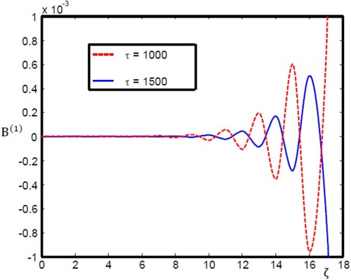Clearly, the OMSSW happens only when the dispersion term dominates over the dissipative parameter. Therefore, we can apply the numerical simulations that illustrate the time evolution of oscillatory magnetosonic shock waves. At τ = 1000, the OMSSW strength increases and goes on ahead more than the oscillations of the OMSSW at τ = 1500.

Figure 1. Temporal evolution of the monotonic magnetosonic shock wave described by Equation (10) with $\text{β}$ = 0.3, ${\epsilon }_0=0.1,$ ${\text{H}}_{\text{e}}$ = 0.1, and${\gamma }_0$ = 0.01.

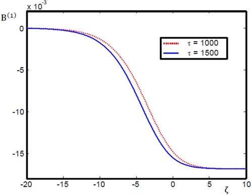
Figure 2. Temporal evolution of the monotonic magnetosonic shock wave with the same physical parameter values as in Figure 1.

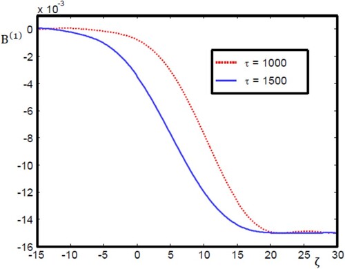
Figure 3. Temporal evolution of the oscillatory magnetosonic shock wave with β = 1.2, ${\epsilon }_0=0.7,$ ${\text{H}}_{\text{e}}$ = 0.3, and${\gamma }_0$ = 0.01.

Let us now focus on the numerical simulations of the dynamical system and the phase portraits that indicate the physical nature of stability/instability around the equilibrium points. That is, the numerical solutions illustrating the nonlinear behaviour of monotonic and oscillatory shock waves. Now, it is instructive to apply the numerical values ${\epsilon }_0=0.7,{\text{H}}_{\text{e}}=0.3,\text{u}=1.2,$ and ${\gamma }_0=0.01$. For complex eigenvalues, Figures 4–6a illustrate the variation in the numerical simulation of the nonlinear oscillatory magnetosonic shock waves (OMSSWs) with different values of the plasma beta $\text{β}(0.2,1.02$ and 1.2, respectively), while all other physical parameters were kept unchanged: the same as displayed in the figure caption (of Figures 4–6a). Furthermore, Figures 4–6b represent, respectively, the phase portraits of Figures 4–6a. At $\text{β}=0.2,$ Figure 4a shows that the nonlinear OMSSWs decrease and the system goes to steady-state behaviour. Furthermore, Figure 5a represents the phase portrait, which indicates that the oscillatory shock structure starting around the equilibrium point ${\text{E}}_1\left(0,0\right)$ converges in a spiral path to the equilibrium point; this behaviour refers to the stability. We can explain this behaviour as follows: based on the above-mentioned numerical values, we can calculate the numerical value of $\theta =-0.195$. Consequently, as $\zeta$ increases in Equation (12), the factor $e^{\theta \zeta }$ has strong effect on the path to becoming a spiral path. Therefore, if $\theta$ < 0, the equilibrium point is stable and then called the spiral stable point. For $\text{β}=1.02,$ Figure 5a illustrates the steady-state behaviour of the dynamical system. To support the numerical investigation of which the result is shown in Figure 5a, one can plot a corresponding phase plane for the steady-state solution of OMSSWs, which demonstrates a closed circular path centred on (0, 0) as displayed in Figure 5b. In this case, $\theta$ is very small ($=-2.8916\text{x}{10}^{-4}),$ the factor ${\text{e}}^{\theta \zeta }$ has no effect on the path. Consequently, the closed trajectories correspond to periodic solutions. In other words, all solutions are therefore periodic and one can expect the equilibrium point to be stable. In the case of $\text{β}=1.2,$ as shown in the bounded oscillations in Figure 6a, one can observe that the fluctuations of the numerical solution increase and the dynamical system goes to increase the oscillations from steady-state. In Figure 6b, the phase plan demonstrates that the OMSSW beginning around the equilibrium point ${\text{E}}_1\left(0,0\right)$ diverges in a spiral path from the equilibrium point, indicating the instability. In this situation, when the numerical value of $\theta =0.2061$, the factor $e^{\theta \zeta }$ has a very strong influence on the path. Therefore, if $\theta$ > 0, the path is spiral and the equilibrium point is unstable, hence called the unstable spiral point. 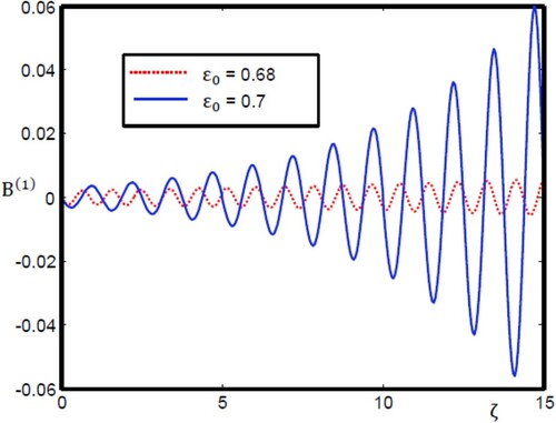Further, Figures 7–9 demonstrate the variation in the numerical simulation of the OMSSWs with different values of the spin magnetization energy ${\epsilon }_0$ $(0.1,0.645$ and 0.7, respectively) maintaining all other parameters unchanged as shown in the caption of corresponding figures. It is highly interesting to point out here that the variation in the nature of OMSSWs displayed in Figures 7–9 are similar to the behaviour of those shown in Figures 4–6, respectively. For ${\epsilon }_0=0.1$, as shown in Figure 7a, the amplitude of magnetosonic wave decreases and the dynamical system move to a steady-state. In Figure 7b, the phase plane points out the stability, the oscillatory shock wave starting around the equilibrium point ${\text{E}}_1\left(0,0\right)$ approaches in a spiral path to the equilibrium point. As displayed in Figure 8a, at ${\epsilon }_0=0.645$, the dynamical system exhibits the steady-state phenomenon. In this situation, the phase plane is described by a closed circular path as seen in Figure 8b. Obviously, at ${\epsilon }_0=0.7$, the bounded fluctuations in Figure 9a of the OMSSWs increase and the system moves to enhance the oscillations from steady state. The phase portrait elucidates the instability of the oscillatory shock wave as shown in Figure 9b. The OMSSW diverges in a spiral path from the equilibrium point ${\text{E}}_1\left(0,0\right)$. It is interesting to mention here that the numerical simulations in Figures 4–9 are consistent with the analytical solutions, which confirm the validity of the numerical code. Let's now investigate the physical aspect of OMSSWs as a result of different values of $\text{β}$ and ${\epsilon }_0$. Figures 10 and 11 illustrate how the plasma beta $\text{β}$ and the normalized Zeeman energy ${\epsilon }_0$ affect, respectively, the OMSSW structure: as the value of $\text{β}$ and ${\epsilon }_0$ increase the OMSSW amplitude increases. In addition, one can observe here that the features of OMSSWs displayed in Figures 12 and 13 are similar to the behaviour of those shown in Figures 10 and 11.

Figure 4. (a) Oscillatory magnetosonic shock wave profile with $\text{β}$ = 0.2, ${\epsilon }_0=0.7,$ ${\text{H}}_{\text{e}}$ = 0.3, and${\gamma }_0$ = 0.01. (b) Phase portrait with the same physical parameter values as in Figure 4 (a).

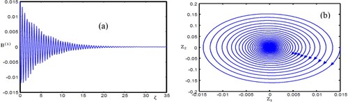
Figure 5. (a) Oscillatory magnetosonic shock wave profile with $\text{β}$ = 1.02, ${\epsilon }_0=0.7,$ ${\text{H}}_{\text{e}}$ = 0.3, and${\gamma }_0$ = 0.01. (b) Phase portrait with the same physical parameter values as in Figure 5 (a).

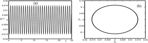
Figure 6. (a) Oscillatory magnetosonic shock wave profile with $\text{β}$ = 1.2, ${\epsilon }_0=0.7,$ ${\text{H}}_{\text{e}}$ = 0.3, and${\gamma }_0$ = 0.01. (b) Phase portrait with the same physical parameter values as in Figure 6 (a).

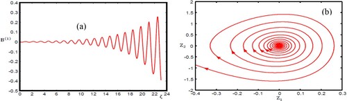
Figure 7. (a) Oscillatory magnetosonic shock wave profile with ${\epsilon }_0=0.1,$ $\text{β}$ = 1.2, ${\text{H}}_{\text{e}}$ = 0.3, and${\gamma }_0$ = 0.01. (b) Phase portrait with the same physical parameter values as in Figure 7 (a).

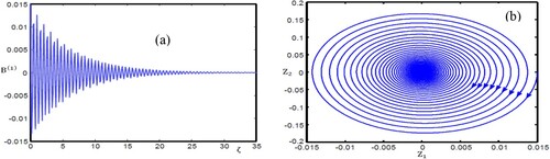
Figure 8. (a) Oscillatory magnetosonic shock wave profile with ${\epsilon }_0=0.645,$ $\text{β}$ = 1.2, ${\text{H}}_{\text{e}}$ = 0.3, and${\gamma }_0$ = 0.01. (b) Phase portrait with the same physical parameter values as in Figure 8 (a).

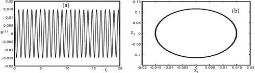
Figure 9. (a) Oscillatory magnetosonic shock wave profile with ${\epsilon }_0=0.7,$ $\text{β}$ = 1.2, ${\text{H}}_{\text{e}}$ = 0.3, and${\gamma }_0$ = 0.01. (b) Phase portrait with the same physical parameter values as in Figure 9 (a).

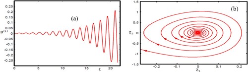
Figure 10. Oscillatory magnetosonic shock wave profile for different values of $\text{β}$ with ${\epsilon }_0=0.7,$ ${\text{H}}_{\text{e}}$ = 0.1, and${\gamma }_0$ = 0.01.

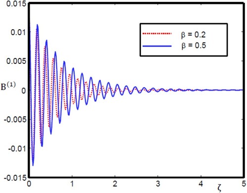
Figure 11. Oscillatory magnetosonic shock wave profile for different values of ${\epsilon }_0$ with $\text{β}=0.5,$ ${\text{H}}_{\text{e}}$ = 0.1, and${\gamma }_0$ = 0.01.

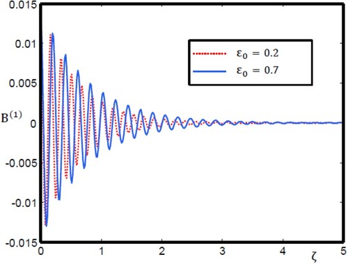
Figure 12. Oscillatory magnetosonic shock wave profile for different values of $\text{β}$ with ${\epsilon }_0=0.7,$ ${\text{H}}_{\text{e}}$ = 0.3, and${\gamma }_0$ = 0.01.

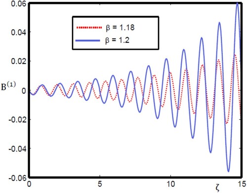
Figure 13. Oscillatory magnetosonic shock wave profile for different values of ${\epsilon }_0$ with $\text{β}=1.2,$ ${\text{H}}_{\text{e}}$ = 0.3, and${\gamma }_0$ = 0.01.

Furthermore, when $\frac{{\gamma }_0^2{\left(1-2{\text{β}\epsilon }_0^2\right)}^2}{{\lambda }^2{\text{H}}_{\text{e}}^2}-2\lambda u>0(\text{i}.\text{e}.,\frac{{\gamma }_0^2{\left(1-2{\text{β}\epsilon }_0^2\right)}^2}{{\text{H}}_{\text{e}}^2{\left(1+0,666\text{β}-3{\text{β}\epsilon }_0^2\right)}^{3/2}}>\text{u})$, using the numerical values of the mentioned physical parameters, one can simply find out that $\frac{{\gamma }_0^2{\left(1-2{\text{β}\epsilon }_0^2\right)}^2}{{\text{H}}_{\text{e}}^2{\left(1+0,666\text{β}-3{\text{β}\epsilon }_0^2\right)}^{3/2}}\approx {10}^{-5}<\text{u}.$ Therefore, the condition $\frac{{\gamma }_0^2{\left(1-2{\text{β}\epsilon }_0^2\right)}^2}{{\lambda }^2{\text{H}}_{\text{e}}^2}-2\lambda u>0$ can never be achieved.

Further, when $\frac{{\gamma }_0^2{\left(1-2{\text{β}\epsilon }_0^2\right)}^2}{{\lambda }^2{\text{H}}_{\text{e}}^2}+2\lambda u>0,$ $(\text{i}.\text{e}.,\frac{-{\gamma }_0^2{\left(1-2{\text{β}\epsilon }_0^2\right)}^2}{{\text{H}}_{\text{e}}^2{\left(1+0,666\text{β}-3{\text{β}\epsilon }_0^2\right)}^{3/2}}>\text{u})$, applying the parameter values ${\epsilon }_0=0.1-0.5,\text{β}=0.1-0.3,{\text{H}}_{\text{e}}=0.1,$ and${\gamma }_0=0.01$, one can simply find out that $\frac{-{\gamma }_0^2{\left(1-2{\text{β}\epsilon }_0^2\right)}^2}{{\text{H}}_{\text{e}}^2{\left(1+0,666\text{β}-3{\text{β}\epsilon }_0^2\right)}^{3/2}}\approx -0.006<\text{u}<0$. 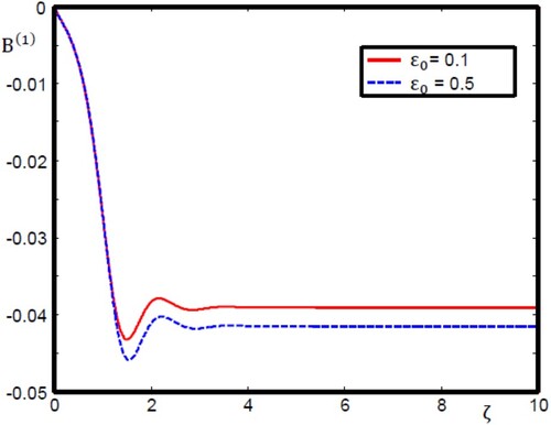Then, the numerical simulation exhibits only a strictly monotonic magnetosonic shock structure. In this case, the MMSSW occurs only when the coefficient of dissipation dominates over the coefficient of dispersion. We now proceed by examining the features of MMSSWs as a consequence of different values of $\text{β}$ and ${\epsilon }_0$. As shown in Figures 14 (15), the amplitudes of the MMSSWs are affected by increasing $\text{β}\left(\text{or }{\epsilon }_0\right)$. It is clear that the strength of the MMSSW decreases (or increases) by increasing the value of $\text{β}\left(\text{or }{\epsilon }_0\right)$. Physically, by increasing$\text{β}\left(\text{or }{\epsilon }_0\right)$, both the quantum statistical effect and the normalized Zeeman energy increase in degenerate Fermi plasmas, which lead to an increase (or a decrease) in the magnitude of the nonlinear coefficient${\text{A}}_1$. Furthermore, Equation (10) (i.e. the analytical solution of MMSSW) demonstrates that the amplitude of the MMSSW is considered to be basically controlled by ${\text{A}}_1$; thus, as the nonlinear coefficient increases (or decrease), the MMSSW potential decreases (or increases). On the other hand, both $\text{β}$ and ${\epsilon }_0$ have slightly influence on the width of the MMSSW. This is because the width of the MMSSW depends on the dispersion confident ${\text{D}}_1$ and the dissipative term ${\text{C}}_1$, which are slightly affected the increase of$\text{β}$ and ${\epsilon }_0$ Figure 15.

Figure 14. Monotonic magnetosonic shock wave profile for different values of $\text{β}$ with ${\epsilon }_0=0.1,$ ${\text{H}}_{\text{e}}$ = 0.1, and ${\gamma }_0$ = 0.01.

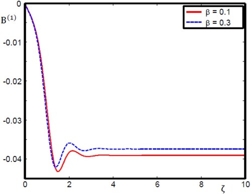
Figure 15. Monotonic magnetosonic shock wave profile for different values of ${\epsilon }_0$ with $\text{β}=0.1,$ ${\text{H}}_{\text{e}}$ = 0.1, and ${\gamma }_0$ = 0.01.

In this work, we have investigated the characteristics of nonlinear MMSSWs and OMSSWs in a degenerate quantum magnetoplasma consisting of ions and spin 1/2 nonrelativistic degenerate electrons. The KdVBE is deduced by employing the well-known reductive perturbation analysis. Interestingly, using the bifurcation analysis, we have discussed and specified the equilibrium points and analytical solutions. Moreover, the fourth order Runge-Kutta method was used to study numerically the nonlinear behaviour of MMSSWs and OMSSWs. Numerical simulations have demonstrated that the physical parameters $\text{β}$ and ${\epsilon }_0$ play central roles in determining the physical nature of MMSSWs and OMSSWs. Therefore, we can conclude that both $\text{β}$ and ${\epsilon }_0$behave like bifurcation parameters. In other words, the numerical values of $\text{β}$ and ${\epsilon }_0$ are responsible for changing the behaviour of OMSSWs from unstable to stable solution and vice versa. Basically, for an advanced comprehension of the physical nature of various systems, one needs to work out more and more studies of the dynamical behaviour by using the dynamical system approach.

Acknowledgments

The authors extend their appreciation to the Deanship of scientific research at King Khalid University for funding this work through research groups pangram under grant number KKU-R.G.P.1/52/39. The authors also thank the editor and his staff for their kind cooperation.

Disclosure statement

No potential conflict of interest was reported by the author(s).

References

- Goossens M, De Groof A. Resonant and phase-mixed magnetohydrodynamic waves in the solar atmosphere. Phys. Plasmas. 2001;8:2371. doi: 10.1063/1.1343090
- Khan SA, Masood W. Linear and nonlinear quantum ion-acoustic waves in dense magnetized electron-positron-ion plasmas. Phys. Plasmas. 2008;15:062301. doi: 10.1063/1.2920273
- El-Shamy EF, Moslem WM, Shukla PK. Head-on collision of ion-acoustic solitary waves in a Thomas–Fermi plasma containing degenerate electrons and positrons. Phys. Lett. A. 2009;374:290–293. doi: 10.1016/j.physleta.2009.10.060
- Masood W, Mirza AM, Nargis S, et al. Ion-acoustic vortices in inhomogeneous and dissipative electron-positron-ion quantum magnetoplasmas. Phys. Plasmas. 2009;16:042308. doi: 10.1063/1.3112707
- El-Bedwehy NA. Freak waves in GaAs semiconductor. Physica B. 2014;442:114–117. doi: 10.1016/j.physb.2014.02.003
- El-Shamy EF. Nonlinear ion-acoustic cnoidal waves in a dense relativistic degenerate magnetoplasma. Phys. Rev. E. 2015;91:033105. doi: 10.1103/PhysRevE.91.033105
- Haas F. Modelling of relativistic ion-acoustic waves in ultra-degenerate plasmas. J. Plasma Phys. 2016;82:705820602. doi: 10.1017/S0022377816001100
- El-Shamy EF, Al-Chouikh RC, El-Depsy A, et al. Nonlinear propagation of electrostatic travelling waves in degenerate dense magnetoplasmas. Plasma Phys. 2016;23:122122. doi: 10.1063/1.4972817
- Islam S, Sultana S, Mamun A A. Envelope solitons in three-component degenerate relativistic quantum plasmas. Phys. Plasmas. 2017;24:092115. doi: 10.1063/1.5001834
- Ostriker JP. Recent developments in the theory of degenerate dwarfs. Annu. Rev. Astron. Astrophys. 1971;9:353–366. doi: 10.1146/annurev.aa.09.090171.002033
- El-Shamy EF, Selim MM, El-Depsy A, et al. Effects of chemical potentials on isothermal ion-acoustic solitary waves and their three dimensional instability in a magnetized ultrarelativistic degenerate multicomponent plasma. Plasma Phys. 2020;27:032101. doi: 10.1063/1.5139885
- Markowich PA, Ringhofer CA, Schmeiser C. Semiconductor equations. Vienna: Springer; 1990.
- Calvayrac F, Reinhard PG, Suraud E, et al. Nonlinear electron dynamics in metal clusters. Phys. Rep. 2000;337:493–578. doi: 10.1016/S0370-1573(00)00043-0
- Stenflo L, Shukla PK, Marklund M. New low-frequency oscillations in quantum dusty plasmas. Europhys. Lett. 2006;74:844–846. doi: 10.1209/epl/i2006-10032-x
- Salamin YI, Hu SX, Hatsagortsyan KZ, et al. Relativistic high-power laser–matter interactions. Phys. Rep. 2006;427:41–155. doi: 10.1016/j.physrep.2006.01.002
- Mourou GA, Tajima T, Bulanov SV. Optics in the relativistic regime. Rev. Mod. Phys. 2006;78:309–371. doi: 10.1103/RevModPhys.78.309
- Becker KH, Schoenbach KH, Eden JG. Microplasmas and applications. J. Phys. D. 2006;39:R55–R70. doi: 10.1088/0022-3727/39/3/R01
- Asseo E. Pair plasma in pulsar magnetospheres. Plasma Phys. Controlled Fusion. 2003;45:853–867. doi: 10.1088/0741-3335/45/6/302
- Kouveliotou C, Dieters S, Strohmayer T, et al. An X-ray pulsar with a superstrong magnetic field in the soft γ-ray repeater SGR1806 – 20. Nature. 1998;393:235–237. doi: 10.1038/30410
- Baring MG, Gonthier PL, Harding AK. Spin-dependent cyclotron decay Rates in strong magnetic fields. Astrophys. J. 2005;630:430–440. doi: 10.1086/431895
- Marklund M, Brodin G. Dynamics of spin- quantum plasmas. Phys. Rev. Lett. 2007;98:025001. doi: 10.1103/PhysRevLett.98.025001
- Brodin G, Marklund M. Spin magnetohydrodynamics. New J. Phys. 2007;9:277. doi: 10.1088/1367-2630/9/8/277
- Marklund M, Eliasson B, Shukla PK. Magnetosonic solitons in a fermionic quantum plasma. Phys. Rev. E. 2007;76:067401. doi: 10.1103/PhysRevE.76.067401
- Brodin G, Marklund M. Spin solitons in magnetized pair plasmas. Phys. Plasmas. 2007;14:112107. doi: 10.1063/1.2793744
- Li SC, Han JN. Magnetosonic waves interactions in a spin- degenerate quantum plasma. Phys. Plasmas. 2014;21:032105. doi: 10.1063/1.4867661
- Han JN, Luo JH, Li SC, et al. Composite nonlinear structure within the magnetosonic soliton interactions in a spin-1/2 degenerate quantum plasma. Phys. Plasmas. 2015;22:062101. doi: 10.1063/1.4921662
- Strogatz SH. Nonlinear dynamics and Chaos. Massachusetts: Perseus Books; 1994.
- Ross SL. Differential equations. New York: John Wiley and Sons; 1984.
- Lakshmanan M, Rajasekar S. Nonlinear dynamics: Integrability, chaos and patterns. Verlag, Berlin: Springer; 2003.
- Guckenheimer J, Holmes P. Nonlinear oscillations, dynamical systems, and bifurcations of vector fields. New York: Springer; 2002.
- Sahu B, Pal B, Poria S, et al. Dynamics of low dimensional model for weakly relativistic Zakharov equations for plasmas. Phys. Plasmas. 2013;20:052303. doi: 10.1063/1.4804340
- Ghosh UN, Mandal PK, Chatterjee P. The roles of non-extensivity and dust concentration as bifurcation parameters in dust-ion acoustic traveling waves in magnetized dusty plasma. Phys. Plasmas. 2014;21:033706. doi: 10.1063/1.4869720
- El-Shamy EF, Mahmoud M, Al-Wadie ES, et al. Excitation and formation conditions of monotonic shock waves in magnetized plasmas with superthermality distributed electrons. J. Korean Phys. Soc. 2019;75:54–62. doi: 10.3938/jkps.75.54
- Zaghbeer SK, Salah HH, Sheta NH, et al. Dust acoustic shock waves in dusty plasma of opposite polarity with non-extensive electron and ion distributions. J. Plasma Phys. 2014;80:517–528. doi: 10.1017/S0022377814000063
- Jordan DW, Smith P. Non-linear ordinary differential equations: Introduction for Scientists and Engineers. London: Oxford University Press; 2007.