Periodic solutions for first-order cubic non-autonomous differential equation with bifurcation analysis

Abstract

This article deals with the development of the number of periodic solutions for ordinary differential equations. We investigated focal values for first-order non-autonomous differential equation for periodic solutions from a fine focus $\mathfrak{z}=0$. Periodic solutions with polynomial coefficients are executed for classes $C_{10,3},C_{10,4},$ and $C_{10,5}.$ Limit cycles are found for both non-homogeneous and homogeneous polynomials with trigonometric coefficients for classes $C_{22,11}$,$C_{24,12}$ and $C_{10,10}$, respectively. We developed a formula ${\varkappa }_{10}$, which is not available in literature. By using our newly developed formula, we succeeded to find highest known multiplicity 10 for the classes $C_{10,3},C_{10,4}$ with algebraic and $C_{10,10},C_{24,12}$ with trigonometric coefficients. We present a variety of polynomial classes along with their bifurcation analysis which confirms the generality and authenticity of the method presented.

Keywords:

• Focal values
• homogeneous and non-homogeneous trigonometric coefficients
• perturbation method

1. Introduction

In real world, in general, most of the known phenomena have the tendency to repeat after some time. There are two main kinds of models: $\left(\mathrm{i}\right)$ The autonomous equation – is the differential in which the dynamic of the system is given by the same map. This kind of systems predicts the evolution without considering many changes along the time. $\left(\mathrm{i}\mathrm{i}\right)$ The non-autonomous equation – the differential equation whose right side, explicitly depends upon time or change. Hence, seasonal influences, controlling, external effects and other mechanisms are considered as non-autonomous models. For example, a linear or nonlinear oscillator can be forced by a periodic external force. The main open problem in the qualitative theory of real planar differential system is the determination of limit cycles. Limit cycles are usually obtained by perturbing the periodic orbits of the centre. In this paper, we are mainly concerned with non-autonomous differential equation for which limit cycles are determined by perturbing the periodic orbits of the centre, for more details, see [1–11].

The problem of studying the limit cycles that can bifurcate from the period annulus surrounding the origin for system of the form (1) $\stackrel{\cdot }{\mathfrak{z}}=\gamma \left(\tau \right){\mathfrak{z}}^3+\delta \left(\tau \right){\mathfrak{z}}^2+\upsilon \left(\tau \right)\mathfrak{z},$(1) with $\mathfrak{z}\mathfrak{=}\mathfrak{0}\mathfrak{,}$ has been extensively considered; see for instance [12–14]. Where $\mathfrak{z}$ is complex-valued; and coefficients are real polynomial in the real variable τ. The question for the number of periodic solutions for non-autonomous differential system continues to attract more interest. Neto in [15] states that for Equation (1(1) $\stackrel{\cdot }{\mathfrak{z}}=\gamma \left(\tau \right){\mathfrak{z}}^3+\delta \left(\tau \right){\mathfrak{z}}^2+\upsilon \left(\tau \right)\mathfrak{z},$(1) ), we are unable to have upper bound for number of periodic solutions until some coefficients are restricted. Also in this paper, our basic focus is to acquire highest periodic solutions for any class of the form of Equation (1(1) $\stackrel{\cdot }{\mathfrak{z}}=\gamma \left(\tau \right){\mathfrak{z}}^3+\delta \left(\tau \right){\mathfrak{z}}^2+\upsilon \left(\tau \right)\mathfrak{z},$(1) ), by using bifurcation method. The Equation (1(1) $\stackrel{\cdot }{\mathfrak{z}}=\gamma \left(\tau \right){\mathfrak{z}}^3+\delta \left(\tau \right){\mathfrak{z}}^2+\upsilon \left(\tau \right)\mathfrak{z},$(1) ), is a part of the equation described in Lloyd [16] as follows: (2) $\stackrel{\cdot }{\mathfrak{z}}=p_0\left(\tau \right){\mathfrak{z}}^n+p_{{}_1}\left(\tau \right){\mathfrak{z}}^{n-1}+p_2\left(\tau \right){\mathfrak{z}}^{n-2}+\cdots +p_n\left(\tau \right).$(2) With the assumption that $p_0\left(\tau \right)=1$ and $p_1\left(\tau \right),\dots ,p_n\left(\tau \right)$ are real-valued periodic continuous functions. This class of equation has received more attention in the literature. It was shown in [17]  that when $p_0\left(\tau \right)=1$, then there are three periodic solutions provided account is taken of multiplicity. For n = 3 Equation (2(2) $\stackrel{\cdot }{\mathfrak{z}}=p_0\left(\tau \right){\mathfrak{z}}^n+p_{{}_1}\left(\tau \right){\mathfrak{z}}^{n-1}+p_2\left(\tau \right){\mathfrak{z}}^{n-2}+\cdots +p_n\left(\tau \right).$(2) ) is known as Abel's differential equation, that is important because of its connection with the well-known Hilbert's sixteenth problem for differential equations. We also refer reader to the article [18], for further information regarding Hilbert's sixteenth problem background and its present status. In general, finding limit cycles is a very difficult problem. The number of limit cycle of a polynomial differential equation in the plane is the main object of the second part of Hilbert's sixteenth problem. When $n\ge 4$ and $p_0\left(\tau \right)=1$, the results of [17] no longer holds; the examples given in Neto [15] can be used to show that there is no upper bound to the periodic solutions. Moreover systems with constant angular velocities can be reduced to polynomial equations. General consequence about the number of periodic solutions can be used to obtain number of limit cycles; for examples see [13,19,20].

Consider that for Equation (1(1) $\stackrel{\cdot }{\mathfrak{z}}=\gamma \left(\tau \right){\mathfrak{z}}^3+\delta \left(\tau \right){\mathfrak{z}}^2+\upsilon \left(\tau \right)\mathfrak{z},$(1) ) there exists $\text{β}\in \mathbb{R}$ such that: $\begin{array}{r}\mathfrak{z}\left(\text{β}\right)=\mathfrak{z}\left(0\right).\end{array}$ These solutions are periodic, even if γ, δ and υ are not themselves periodic. The solution satisfying $\mathfrak{z}\left(\text{β}\right)=\mathfrak{z}\left(0\right),$ are called periodic orbits of the equation. To find maximum number of periodic solution for Equation (1(1) $\stackrel{\cdot }{\mathfrak{z}}=\gamma \left(\tau \right){\mathfrak{z}}^3+\delta \left(\tau \right){\mathfrak{z}}^2+\upsilon \left(\tau \right)\mathfrak{z},$(1) ), complexified form is used. This is because, the number of zeros in a bounded region of the complex plane cannot be changed by any small perturbation of the coefficients. For more detail, see [12,15,17]. The periodic orbits that are isolated in the set of all periodic orbits are usually called limit cycle. Limit cycles bifurcate out of the fine focus $\mathfrak{z}=0$ when the coefficients of γ and δ are slightly perturb in bifurcation method. If for Equation (1(1) $\stackrel{\cdot }{\mathfrak{z}}=\gamma \left(\tau \right){\mathfrak{z}}^3+\delta \left(\tau \right){\mathfrak{z}}^2+\upsilon \left(\tau \right)\mathfrak{z},$(1) ) multiplicity $\mu >1,$ as was described in [12], we could reduce the Equation (1(1) $\stackrel{\cdot }{\mathfrak{z}}=\gamma \left(\tau \right){\mathfrak{z}}^3+\delta \left(\tau \right){\mathfrak{z}}^2+\upsilon \left(\tau \right)\mathfrak{z},$(1) ) to the form as follows: (3) $\stackrel{\cdot }{\mathfrak{z}}=\gamma \left(\tau \right){\mathfrak{z}}^3+\delta \left(\tau \right){\mathfrak{z}}^2.$(3) Here γ and δ may be polynomials $\left(\mathrm{i}\right)$ in τ $\left(\mathrm{i}\mathrm{i}\right)$ in $cos\tau$ and $sin\tau$ (trigonometric functions). The functions ${\xi }_i\left(\tau \right),$ for i>1 are calculated by utilizing the relation: (4) ${\stackrel{\cdot }{\xi }}_i=\gamma \sum _{\stackrel{j+k+l=i}{{}_{j,k,l\ge 1}}}{\xi }_j{\xi }_k{\xi }_l+\delta \sum _{\stackrel{j+k=i}{j,k\ge 1}}{\xi }_j{\xi }_k.$(4) With ${\xi }_1\left(\tau \right)=1$. However as ${}^{″}{i}^{″}$ increases, certain calculations become tremendously complicated because of integration by parts, used in it. Assume that ${\varkappa }_i=$ ${\xi }_i\left(\text{β}\right),$ at that point $\varkappa =i$ if ${\varkappa }_1=1$ and ${\varkappa }_k=0$ for $2\le k\le i-2$ but ${\varkappa }_i\ne 0$ these ${\varkappa }_{i^{\stackrel{´}{}}s}$ are known as focal values, given in Section 2. For $i\le 8$ functions ${\xi }_i\left(\tau \right)$ and ${\varkappa }_i$ are given in [12], for i = 9 Yasmin in [21] had calculated ${\xi }_9\left(\tau \right)$ and ${\varkappa }_9$. For $i=10,$  we have calculated ${\xi }_{10}\left(\tau \right)$ and ${\varkappa }_{10}.$ It also gives attention to the readers that one may calculate the next formulas by substituting the value of i>10, in Equation (4(4) ${\stackrel{\cdot }{\xi }}_i=\gamma \sum _{\stackrel{j+k+l=i}{{}_{j,k,l\ge 1}}}{\xi }_j{\xi }_k{\xi }_l+\delta \sum _{\stackrel{j+k=i}{j,k\ge 1}}{\xi }_j{\xi }_k.$(4) ). Due to which, one may be able to compute the maximum periodic solutions greater than ten.

In Section 3, perturbation techniques and isolation conditions for centre are given. Main results are presented in Section 4 and some conclusions are given in Section 5.

2. Development of some essential formulas

For Equation (4(4) ${\stackrel{\cdot }{\xi }}_i=\gamma \sum _{\stackrel{j+k+l=i}{{}_{j,k,l\ge 1}}}{\xi }_j{\xi }_k{\xi }_l+\delta \sum _{\stackrel{j+k=i}{j,k\ge 1}}{\xi }_j{\xi }_k.$(4) ), Alwash in [12] gives functions ${\xi }_i\left(\tau \right)$ and ${\varkappa }_i,$ for $2\le i\le 8$ and Yasmin in [21] had calculated ${\xi }_9\left(\tau \right)$ and ${\varkappa }_9.$ For i = 10 we have calculated ${\xi }_{10}\left(\tau \right)$ and ${\varkappa }_{10},$ presented in Theorems 2.1 and 2.2. To develop Algorithm for various classes, we use computer Algebra Language Maple, which can be used to calculate periodic solutions by using following theorems.

Theorem 2.1

For Equation (4(4) ${\stackrel{\cdot }{\xi }}_i=\gamma \sum _{\stackrel{j+k+l=i}{{}_{j,k,l\ge 1}}}{\xi }_j{\xi }_k{\xi }_l+\delta \sum _{\stackrel{j+k=i}{j,k\ge 1}}{\xi }_j{\xi }_k.$(4) ) conclusive functions ${\xi }_2,{\xi }_3,\dots ,{\xi }_8$ are given in [12]. And conclusive function ${\xi }_9$ and ${\xi }_{10}$ are given as follows:

By using these functions, we have theorem 2 that enables us to find the maximum multiplicity in which integral is like $\int \gamma \left(\tau \right)\overline{\delta \left(\tau \right)}\mathrm{d}\tau .$  Here bar ${}^{″}{-}^{″}$ shows integral of the form $\overline{\delta \left(\tau \right)}=\int \delta \left(\tau \right)\mathrm{d}\tau ,$ and is indefinite. This is the main theorem given by Alwash in [12] with which we are able to calculate the multiplicity.

Theorem 2.2

The solution $\mathfrak{z}=0$ of (3(3) $\stackrel{\cdot }{\mathfrak{z}}=\gamma \left(\tau \right){\mathfrak{z}}^3+\delta \left(\tau \right){\mathfrak{z}}^2.$(3) ) has a multiplicity k, wherever $2\le k\le 10$ iff ${\varkappa }_n=0$ for $2\le n\le k-1$ and ${\varkappa }_n\ne 0$ where

${\varkappa }_2={\int }_0^{\text{β}}\delta ,$

${\varkappa }_3={\int }_0^{\text{β}}\gamma ,$

${\varkappa }_4={\int }_0^{\text{β}}\gamma \overline{\delta },$

${\varkappa }_5={\int }_0^{\text{β}}\gamma {\overline{\delta }}^2,$

${\varkappa }_6={\int }_0^{\text{β}}\gamma {\overline{\delta }}^3-\frac{1}{2}{\overline{\gamma }}^2\delta ,$

${\varkappa }_7={\int }_0^{\text{β}}\gamma {\overline{\delta }}^4+2\gamma {\overline{\delta }}^2\overline{\gamma },$

${\varkappa }_8={\int }_0^{\text{β}}\gamma {\overline{\delta }}^5+3\gamma {\overline{\delta }}^3\overline{\gamma }+\gamma {\overline{\delta }}^2\overline{\overline{\delta }\gamma }-\frac{1}{2}{\overline{\gamma }}^3\delta ,$

${\varkappa }_9={\int }_0^{\text{β}}\gamma {\overline{\delta }}^6-5\gamma {\overline{\delta }}^4\overline{\gamma }-2{\overline{\delta }}^3\overline{\delta \overline{\gamma }}+20\overline{\delta {\overline{\gamma }}^2}+2\overline{\delta \overline{\gamma }}\delta {\overline{\gamma }}^2,$

and $\begin{array}{rl}{\varkappa }_{10}& ={\int }_0^{\text{β}}\gamma {\overline{\delta }}^7-\frac{1235}{6}\gamma \overline{\gamma }{\overline{\delta }}^5-\frac{970}{3}\gamma {\overline{\gamma }}^2{\overline{\delta }}^3-237\delta {\overline{\delta }}^2{\overline{\gamma }}^3\\ & -24\gamma {\overline{\gamma }}^2\delta {\overline{\delta }}^2-70\overline{\gamma }{\overline{\delta }}^3{\gamma }^2-21{\overline{\gamma }}^4\delta -74\gamma {\overline{\gamma }}^3\overline{\delta }\\ & +\frac{5}{2}{\overline{\gamma }}^2\delta {\overline{\delta }}^4+32{\overline{\delta }}^4\gamma \overline{\delta \overline{\gamma }}\\ & -16\delta {\overline{\delta }}^4\overline{\gamma }-15{\overline{\delta }}^5{\gamma }^2-36\delta \overline{\delta }{\overline{\gamma }}^2\overline{\delta \overline{\gamma }}-8\delta {\overline{\delta }}^4\gamma \overline{\gamma }.\end{array}$

3. Bifurcation and isolation conditions for centre

In this section, we describe some conditions for centre. From Theorem 2.2, we find maximum periodic solutions for different classes of non-autonomous differential equation of the form as (1(1) $\stackrel{\cdot }{\mathfrak{z}}=\gamma \left(\tau \right){\mathfrak{z}}^3+\delta \left(\tau \right){\mathfrak{z}}^2+\upsilon \left(\tau \right)\mathfrak{z},$(1) ). Stopping criteria is defined for calculating maximum multiplicity ${\varkappa }_k.$ Now, some suitable conditions sufficient for $\mathfrak{z}=0$ as a centre are given below in the form of theorems and corollaries as:

Theorem 3.1

Consider that there are continuous functions f, g defined on $I=\sigma \left(\right[0,\alpha \left]\right)$ and differentiable function σ with$\sigma \left(\alpha \right)=\sigma \left(0\right)$ such that: $\begin{array}{rl}\gamma \left(\tau \right)& =f\left(\sigma \left(\tau \right)\right)\stackrel{\cdot }{\sigma }\\ \delta \left(\tau \right)& =g\left(\sigma \left(\tau \right)\right)\stackrel{\cdot }{\sigma },\end{array}$ then the origin is a centre for (3(3) $\stackrel{\cdot }{\mathfrak{z}}=\gamma \left(\tau \right){\mathfrak{z}}^3+\delta \left(\tau \right){\mathfrak{z}}^2.$(3) ).

Corollary 3.1

The origin is a centre for Equation (3(3) $\stackrel{\cdot }{\mathfrak{z}}=\gamma \left(\tau \right){\mathfrak{z}}^3+\delta \left(\tau \right){\mathfrak{z}}^2.$(3) ). If γ is a constant multiple of δ and ${\int }_0^{\text{β}}\delta \left(\tau \right)\mathrm{d}\tau =0.$

Corollary 3.2

If any δ or γ is identically 0 and other has mean value zero then the origin is a centre.

Corollary 3.3

For odd continuously differentiable functions γ and δ of period ω. The origin is a centre.

Corollary 3.4

Consider for continuously differentiable functions γ and δ of period ω and there exist $\theta \in [0,\omega ]$ such that $\gamma (\theta -\tau )=-\gamma \left(\tau \right),\delta (\theta -\tau )=-\delta \left(\tau \right).$ The origin is a centre.

After determining the maximum multiplicity, which we called μ, now we have to make series of perturbation of the coefficients, every one of which results one periodic solution to come out of origin. We briefly explain it here, for more detail, see [12,16].

For this, suppose equation of the form (3(3) $\stackrel{\cdot }{\mathfrak{z}}=\gamma \left(\tau \right){\mathfrak{z}}^3+\delta \left(\tau \right){\mathfrak{z}}^2.$(3) ), having multiplicity $\mu =j$ $($suppose). Let $\mathcal{U}$ be in the region nearby 0 in the complex plane containing no periodic solution except $\mathfrak{z}=0$. From theorem (2.4) in [12], the initial point which is contained in $\mathcal{U}$ remained fixed with respect to the total number of periodic solutions. Having the restriction that perturbation of the coefficients consider small enough. Our goal is to get ${\varkappa }_2={\varkappa }_3=\cdots ={\varkappa }_{j-2}=0$ but ${\varkappa }_{j-1}\ne 0$ by perturbing and making suitable choices of γ and δ, if possible. Obviously the most effective solution in $\mathcal{U}$ and ψ are zero solution while we get periodic solution $\psi \left(\tau \right)$ where $\psi \left(0\right)\in \mathcal{U}$ as non-trivial solution. By considering the underlying fact that the complex solutions always appear in conjugate pair, so we can say that ψ is real. Let now ${\mathcal{U}}_1$ and ${\mathcal{V}}_1$ are neighbourhood of zero and ψ, respectively, such that ${\mathcal{V}}_1\cup {\mathcal{U}}_1\subset \mathcal{U}$ and ${\mathcal{V}}_1\cap {\mathcal{U}}_1=\phi$. The periodic solutions around ${\mathcal{V}}_1$ and ${\mathcal{U}}_1$ are preserved when we take small perturbation in presented coefficients. By applying same procedure as above our choice is to perturb the coefficients such that ${\varkappa }_k=0$ for $k=2,3,\dots ,j-3$ but ${\varkappa }_{j-2}\ne 0,$ So we get $\mu =j-2$. By applying that procedure we get two non-trivial real periodic solutions with zero solution having multiplicity $j-2.$ Continuously, in this way we ends up for Equation (3(3) $\stackrel{\cdot }{\mathfrak{z}}=\gamma \left(\tau \right){\mathfrak{z}}^3+\delta \left(\tau \right){\mathfrak{z}}^2.$(3) ) having $\mu =2,$ and j−2 distinct non-trivial (other than zero) real periodic solutions.

Remark 3.1

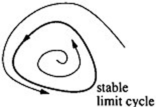
In the perturbation techniques defined above; the full complement of $(j-2)$ real periodic solutions fails to yield, if it so happens that there is j<k such that ${\varkappa }_j=0$ whenever ${\varkappa }_{j-1}=0.$ This happens when the multiplicity is necessarily odd. However, for the number of real periodic solutions, we can say from “exchange of stability” argument that, If multiplicity μ is even, the origin is stable ${\varkappa }_{\mu }<0$ and unstable if ${\varkappa }_{\mu }>0.$ If μ is odd, then the origin is stable on the right and unstable on the left if ${\varkappa }_{\mu }<0,$ while it is stable on the left and unstable on the right if ${\varkappa }_{\mu }>0.$

4. Main results

4.1. Polynomial coefficients for classes $C_{10,3}$, $C_{10,4}$ and $C_{10,5}$

To compute the higher periodic solutions, we use programming language Maple18. Moreover, method for calculating periodic solution involves integration by parts, which is very time consuming as the multiplicity increases. For the polynomial ${}^{″}{\tau }^{″}$ consider $C_{p,q}$ indicates the class of equation of the form (3(3) $\stackrel{\cdot }{\mathfrak{z}}=\gamma \left(\tau \right){\mathfrak{z}}^3+\delta \left(\tau \right){\mathfrak{z}}^2.$(3) ) with degree$p$ & q for γ and δ, respectively, for example, see [14,22–24], the above-mentioned classes are presented below in the form of theorems. The verification of the following theorems, with which we are concerned, stems form a sequence of papers published by Alwash in [12,13,19].

Theorem 4.1

Consider the class $C_{10,3}$ for Equation (3(3) $\stackrel{\cdot }{\mathfrak{z}}=\gamma \left(\tau \right){\mathfrak{z}}^3+\delta \left(\tau \right){\mathfrak{z}}^2.$(3) ), with $\begin{array}{rl}& \gamma \left(\tau \right)=a+b\tau +\mathrm{d}{\tau }^3+e{\tau }^4+h{\tau }^7+k{\tau }^{10}.\\ & \delta \left(\tau \right)=m+p{\tau }^3.\end{array}$ Then we conclude ${\mu }_{max}\left(C_{10,3}\right)\ge 10.$

Proof.

Using Theorem 2.2, we take: $\begin{array}{rl}& {\varkappa }_2=m+\frac{1}{4}p,\\ & {\varkappa }_3=a+\frac{1}{2}b+\frac{1}{4}d+\frac{1}{5}e+\frac{1}{8}h+\frac{1}{11}k.\end{array}$ Thus multiplicity of $\mathfrak{z}=0$ is $\mu =2,$ if ${\varkappa }_2\ne 0.$ And multiplicity $\mu =3,$ if ${\varkappa }_2=0$ but ${\varkappa }_3\ne 0$. If ${\varkappa }_2={\varkappa }_3=0,$ then by using value of ${}^{″}{m}^{″}$ and ${}^{″}{a}^{″},$ $\gamma \left(\tau \right)$  and $\delta \left(\tau \right)$ are as follows: (5) $\begin{array}{rl}\gamma \left(\tau \right)& =b(\tau -\frac{1}{2})+d\left({\tau }^3-\frac{1}{4}\right)+e\left({\tau }^4-\frac{1}{5}\right)+\\ & +h\left({\tau }^7-\frac{1}{8}\right)+k\left({\tau }^{10}-\frac{1}{11}\right),\end{array}$(5) (6) $\begin{array}{rl}\delta \left(\tau \right)& =p\left({\tau }^3-\frac{1}{4}\right).\end{array}$(6) Also we compute ${\varkappa }_4$ as given below: $\begin{array}{r}{\varkappa }_4=-\frac{p(-420k-385h-176e+660b)}{158400}.\end{array}$ If ${\varkappa }_4=0,$ then either p = 0 or: (7) $k=-\frac{385}{420}h-\frac{176}{420}e+\frac{660}{420}b.$(7) If $p=0,$ then $\delta \left(\tau \right)=0$ and for${\varkappa }_3=0,$ it means that mean value of $\gamma \left(\tau \right)$ is zero. Thus, origin is a centre from Corollary 3.2. So, consider that $p\ne 0$. Now if (7(7) $k=-\frac{385}{420}h-\frac{176}{420}e+\frac{660}{420}b.$(7) ) holds then ${\varkappa }_5$ is given as: $\begin{array}{r}{\varkappa }_5=\frac{p^2(-1127h-880e+108b)}{119508480}.\end{array}$ If ${\varkappa }_5=0,$ then as already considered $p\ne 0$ implies: (8) $h=-\frac{880}{1127}e+\frac{108}{1127}b.$(8) And by using (8(8) $h=-\frac{880}{1127}e+\frac{108}{1127}b.$(8) ) we take ${\varkappa }_6$ as: $\begin{array}{r}{\varkappa }_6=-\frac{243p(e+5b)(36680b+17595p^2-2048e)}{649295751104000}.\end{array}$ If ${\varkappa }_6=0,$ as we already supposed $p\ne 0$ either e = −5b or (9) $e=\frac{36680}{2048}b+\frac{17595}{2048}{p}^2.$(9) If $e=-5b,$ then $h=4b,k=0,$ and Equations (5) and (6(6) $\begin{array}{rl}\delta \left(\tau \right)& =p\left({\tau }^3-\frac{1}{4}\right).\end{array}$(6) ) take the following form: $\begin{array}{rl}\gamma \left(\tau \right)& =d\left({\tau }^3-\frac{1}{4}\right)+b\left(4{\tau }^7-5{\tau }^4+t\right),\\ \delta \left(\tau \right)& =p\left({\tau }^3-\frac{1}{4}\right).\end{array}$ Let $\sigma \left(\tau \right)=\left({\tau }^4/4\right)-\left(\tau /4\right)$ then, $\stackrel{\cdot }{\sigma }\left(\tau \right)={\tau }^3-\frac{1}{4}$, also $\sigma \left(0\right)=\sigma \left(1\right).$ So, we write above equations as: $\begin{array}{rl}\gamma \left(\tau \right)& =\left[d+f\left(4{\tau }^4-4\tau \right)\right]\stackrel{\cdot }{\sigma }\left(\tau \right),\\ \delta \left(\tau \right)& =p\stackrel{\cdot }{\sigma }\left(\tau \right).\end{array}$ Thus, from Theorem 3.1, origin is the centre with $f\left(\sigma \right)=[d+f(4{\tau }^4-4\tau \left)\right],$ and $g\left(\sigma \right)=p.$ So, we take $e\ne -5b.$ If (9(9) $e=\frac{36680}{2048}b+\frac{17595}{2048}{p}^2.$(9) ) holds then we compute ${\varkappa }_7$ as: $\begin{array}{r}{\varkappa }_7=-\frac{\begin{array}{c}{p}^2(3p^2+8b)(13670440264b\\ +5589889019p^2+1199245824d)\end{array}}{47695612493168640}.\end{array}$ If ${\varkappa }_7=0$ recalling that $p\ne 0$ then either $b=-\frac{3}{8}{p}^2$ or: (10) $b=-\frac{5589889019}{13670440264}{p}^2-\frac{1199245824}{13670440264}d.$(10) If $b=-\frac{3}{8}{p}^2$ then from Theorem 3.1, origin is the centre with $f\left(\sigma \right)=\left[d+p^2\left(-\frac{3}{2}{\tau }^4+\frac{3}{2}\tau \right)\right]$ and $g\left(\sigma \right)=p.$ So, consider that $b\ne -\frac{3}{8}{p}^2.$ By using (10(10) $b=-\frac{5589889019}{13670440264}{p}^2-\frac{1199245824}{13670440264}d.$(10) ), we calculate ${\varkappa }_8$ as: $\begin{array}{r}{\varkappa }_8=\frac{p(258635p^2+669222d)\mathrm{\Psi }}{\begin{array}{c}43463316928873540928239207930\\ 410620419276800\end{array}}.\end{array}$ Where the value of Ψ is, $\begin{array}{rl}\mathrm{\Psi }& =-7526084232904678336920240879p^4\\ & -8751871539611598818810702d{p}^2\\ & +926676854534594320425774d^2.\end{array}$ Now, if ${\varkappa }_8=0$ then either $\mathrm{\Psi }=0$ or  (11) $d=-\frac{258635}{669222}{p}^2.$(11) Because $p\ne 0$. If (11(11) $d=-\frac{258635}{669222}{p}^2.$(11) ) holds but $\mathrm{\Psi }\ne 0,p\ne 0$ then we compute ${\varkappa }_9$ as: $\begin{array}{r}{\varkappa }_9=-\frac{p^5(2111147084238400+21174293979747p)}{16152297100357017600}.\end{array}$ If ${\varkappa }_9=0$ then, as $p\ne 0$ considered above results $p^5\ne 0$, we take value of p as: (12) $p=-\frac{2111147084238400}{21174293979747}.$(12) If Equation (11(11) $d=-\frac{258635}{669222}{p}^2.$(11) ) $\ne 0,$ $p\ne 0,$ but $\mathrm{\Psi }=0$ holds then $d=y_i{p}^2$ for i = 1, 2 with $y_1=94.9656479174,y_2=-\mathrm{85.5212860619.}$ If (12(12) $p=-\frac{2111147084238400}{21174293979747}.$(12) ) holds then we calculate ${\varkappa }_{10}$ as: $\begin{array}{r}{\varkappa }_{10}=-\frac{\begin{array}{c}933514281331515930245682043545\\ 2503033986414088791807100\\ 1783779417421204958773850815232\end{array}}{\begin{array}{c}57938965448794294696572655129721\\ 433211790606681649184446\\ 0616391273770091215\end{array}}.\end{array}$ Here ${\varkappa }_{10}$ is equal to constant number which is non-zero. Hence, we conclude that multiplicity of class $C_{10,3}$ is 10 i.e. ${\mu }_{max}\left(C_{10,3}\right)\ge 10$. As the maximum multiplicity is 10 (even) and is also negative. So, from Remark 3.1, the periodic solutions are stable (Figure 1).

Figure 1. Stability of Class $C_{10,3}$.

Theorem 4.2

For Equation (3(3) $\stackrel{\cdot }{\mathfrak{z}}=\gamma \left(\tau \right){\mathfrak{z}}^3+\delta \left(\tau \right){\mathfrak{z}}^2.$(3) ), with

$\begin{array}{rl}\gamma \left(\tau \right)& =\frac{258635}{2676888}{\left(-\frac{2111147084238400}{21174293979747}+{ϵ}_1\right)}^2\\ & +\frac{239433569}{23923270462}{ϵ}_2-\frac{37179}{12544}{ϵ}_3-\frac{729}{5635}{ϵ}_4\\ & -\frac{1}{24}{ϵ}_5-\frac{1}{11}{ϵ}_6+{ϵ}_7+(-\frac{3}{8}(-\frac{2111147084238400}{21174293979747}+{ϵ}_1{)}^2\\ & -\frac{149905728}{1708805033}{ϵ}_2+{ϵ}_3)\tau +(-\frac{258635}{669222}\\ & \times {\left(-\frac{2111147084238400}{21174293979747}+{ϵ}_1\right)}^2+{ϵ}_2){\tau }^3\\ & +(\frac{15}{8}{\left(-\frac{211114704238400}{21174293979747}+{ϵ}_1\right)}^2\\ & -\frac{1073940045}{6835220132}{ϵ}_2+\frac{4585}{256}{ϵ}_3+{ϵ}_4){\tau }^4\\ & +(-\frac{3}{2}(-\frac{2111147084238400}{21174293979747}+{ϵ}_1{)}^2\\ & +\frac{14574316716}{11961635231}{ϵ}_2-\frac{10889}{784}{ϵ}_3-\frac{880}{1127}{ϵ}_4+{ϵ}_5){\tau }^7\\ & +(-\frac{37543542}{62559749}{ϵ}_2+\frac{10659}{1568}{ϵ}_3+\frac{1672}{5635}{ϵ}_4-\frac{11}{12}{ϵ}_5+{ϵ}_6){\tau }^{10}.\end{array}$

and (13) $\begin{array}{rl}\delta \left(\tau \right)& =\frac{527786771059600}{21174293979747}-\frac{1}{4}{ϵ}_1+{ϵ}_8\\ & +\left(-\frac{2111147084238400}{21174293979747}+{ϵ}_1\right){\tau }^3.\end{array}$(13) Choose ${ϵ}_p$ for $1\le p\le 8$ to be non-zero and small as compared to ${ϵ}_{p-1}$. Then there exist eight real non-trivial periodic solutions for Equation (3(3) $\stackrel{\cdot }{\mathfrak{z}}=\gamma \left(\tau \right){\mathfrak{z}}^3+\delta \left(\tau \right){\mathfrak{z}}^2.$(3) ).

Proof.

If substitute${ϵ}_p=0,\mathrm{\forall }p=1,2,\dots ,8$ and coefficients are as given Theorem 4.2. So, multiplicity of the origin $\varkappa$ is 10. Now, choose ${ϵ}_1\ne 0$ and ${ϵ}_p=0$ for $2\le p\le 8$ then it can be easily seen that ${\varkappa }_9$ is constant multiple of ${ϵ}_1$, but${\varkappa }_2={\varkappa }_3=\cdots ={\varkappa }_7={\varkappa }_8=0.$ So, the multiplicity reduces by one and $\varkappa =9.$ For that reason, one periodic solutions bifurcate out of the origin. Now set ${ϵ}_1\ne 0,$ ${ϵ}_2\ne 0$ and ${ϵ}_p=0$ for $3\le p\le 8$ then we have ${\varkappa }_p=0$ for $p=2,3,\dots ,7.$ But ${\varkappa }_8$ results in form of ${ϵ}_2$ with some constant multiple. So, $\varkappa =8.$ Now, set ${ϵ}_1\ne 0,$ ${ϵ}_2\ne 0,{ϵ}_3\ne 0$ and ${ϵ}_p=0$ for $4\le p\le 8$ then we have ${\varkappa }_p=0$ for $p=2,3,\dots ,6.$ But ${\varkappa }_7$ results in form of ${ϵ}_3$ with some constant multiple. If ${ϵ}_2$ is sufficient small then there are two non-trivial real periodic solutions. Further moving on present way, we own eight real periodic non-trivial solutions.

Corollary 4.1

For an equation (14) $\stackrel{\cdot }{\mathfrak{z}}=\gamma \left(\tau \right){\mathfrak{z}}^3+\delta \left(\tau \right){\mathfrak{z}}^2+\nu +\upsilon .$(14) If $\gamma \left(\tau \right),\delta \left(\tau \right)$ are as given in Theorem 4.2 and $\nu ,\upsilon$ are small enough, Equation (14(14) $\stackrel{\cdot }{\mathfrak{z}}=\gamma \left(\tau \right){\mathfrak{z}}^3+\delta \left(\tau \right){\mathfrak{z}}^2+\nu +\upsilon .$(14) ) has 10 real periodic solutions.

Proof.

Given that $\nu =0,$ $\upsilon =0$ and $\mu =2$ then, (14(14) $\stackrel{\cdot }{\mathfrak{z}}=\gamma \left(\tau \right){\mathfrak{z}}^3+\delta \left(\tau \right){\mathfrak{z}}^2+\nu +\upsilon .$(14) ) have eight real periodic solution. If $\nu \ne 0$ but enough small then $\mu =1,$ also using the same arguments as above, we have nine periodic solutions. These are distinct and other than 0, $\mathfrak{z}=0$ is another solution. Thus we take 10 real periodic solutions.

Theorem 4.3

Consider the class $C_{10,4}$ for Equation (3(3) $\stackrel{\cdot }{\mathfrak{z}}=\gamma \left(\tau \right){\mathfrak{z}}^3+\delta \left(\tau \right){\mathfrak{z}}^2.$(3) ), with $\begin{array}{rl}\gamma \left(\tau \right)& =a+b\tau +e{\tau }^4+f{\tau }^5+j{\tau }^9+k{\tau }^{10}.\\ \delta \left(\tau \right)& =m+q{\tau }^4.\end{array}$ Then we concluded that ${\mu }_{max}\left(C_{10,4}\right)\ge 10.$

Proof.

Using Theorem 2.2, we take $\begin{array}{rl}& {\varkappa }_2=m+\frac{1}{5}q,\\ & {\varkappa }_3=a+\frac{1}{2}b+\frac{1}{5}e+\frac{1}{6}f+\frac{1}{10}j+\frac{1}{11}k.\end{array}$ Thus multiplicity of $\mathfrak{z}=0$ is $\mu =2$ if ${\varkappa }_2\ne 0.$ And multiplicity $\mu =3$ if ${\varkappa }_2=0$ but ${\varkappa }_3\ne 0$. If ${\varkappa }_2={\varkappa }_3=0;$ then, $\gamma \left(\tau \right)$ and $\delta \left(\tau \right)$ takes the form as follows: (15) $\begin{array}{rl}\gamma \left(\tau \right)& =b(\tau -\frac{1}{2})+e\left({\tau }^4-\frac{1}{5}\right)+f\left({\tau }^5-\frac{1}{6}\right)\\ & +j\left({\tau }^9-\frac{1}{10}\right)+k\left({\tau }^{10}-\frac{1}{11}\right),\end{array}$(15) (16) $\begin{array}{rl}\delta \left(\tau \right)& =m\left({\tau }^4-\frac{1}{5}\right).\end{array}$(16) And we compute ${\varkappa }_4$ as given below $\begin{array}{r}{\varkappa }_4=-\frac{q(-525k-504j-200f+1320b)}{277200}.\end{array}$ If ${\varkappa }_4=0$ then either q = 0 or (17) $k=-\frac{504}{525}j-\frac{200}{525}f+\frac{1320}{525}b.$(17) If q = 0 then $\delta \left(\tau \right)=0$ and for ${\varkappa }_3=0,$ it shows that mean value of $\gamma \left(\tau \right)$ is zero. Thus origin is a centre from Corollary 3.2. So consider that $q\ne 0$. Now if (17(17) $k=-\frac{504}{525}j-\frac{200}{525}f+\frac{1320}{525}b.$(17) ) holds then ${\varkappa }_5$ is calculated as: $\begin{array}{r}{\varkappa }_5=-\frac{q^2(15414j+26375f+81180b)}{7861854000}.\end{array}$ If ${\varkappa }_5=0$ then as we already considered $q\ne 0$ implies: (18) $j=-\frac{26375}{15414}f-\frac{81180}{15414}b.$(18) By using (18(18) $j=-\frac{26375}{15414}f-\frac{81180}{15414}b.$(18) ) we take ${\varkappa }_6$ as follows: $\begin{array}{r}{\varkappa }_6=-\frac{\begin{array}{c}q(f+6b)(649493400b+179590716q^2\\ -16466875f)\end{array}}{52171649245497600}.\end{array}$ If ${\varkappa }_6=0$ then as we already considered $q\ne 0$ either f = −6b or (19) $f=\frac{649493400}{16466875}b+\frac{179590716}{16466875}{q}^2.$(19) If f = −6b then (18(18) $j=-\frac{26375}{15414}f-\frac{81180}{15414}b.$(18) ) gives $j=5b,$ and (17(17) $k=-\frac{504}{525}j-\frac{200}{525}f+\frac{1320}{525}b.$(17) ) gives $k=0$. By using these values, Equations (15(15) $\begin{array}{rl}\gamma \left(\tau \right)& =b(\tau -\frac{1}{2})+e\left({\tau }^4-\frac{1}{5}\right)+f\left({\tau }^5-\frac{1}{6}\right)\\ & +j\left({\tau }^9-\frac{1}{10}\right)+k\left({\tau }^{10}-\frac{1}{11}\right),\end{array}$(15) ) and (16(16) $\begin{array}{rl}\delta \left(\tau \right)& =m\left({\tau }^4-\frac{1}{5}\right).\end{array}$(16) ) can be written in the following form as: $\begin{array}{rl}& \gamma \left(\tau \right)=e\left({\tau }^4-\frac{1}{5}\right)+b\left(5{\tau }^9-6{\tau }^5+\tau \right),\\ & \delta \left(\tau \right)=m\left({\tau }^4-\frac{1}{5}\right).\end{array}$ Let $\sigma \left(\tau \right)={\tau }^5-\tau$ then $\stackrel{\cdot }{\sigma }\left(\tau \right)=5{\tau }^4-1$. Also $\sigma \left(0\right)=\sigma \left(1\right).$ Hence, we can write above equations as: $\begin{array}{rl}& \gamma \left(\tau \right)=\frac{1}{5}\left[e+b\left(5{\tau }^5-5\tau \right)\right]\stackrel{\cdot }{\sigma },\\ & \delta \left(\tau \right)=\frac{m}{5}\stackrel{\cdot }{\sigma }.\end{array}$ Thus from Theorem 3.1, origin is the centre with $f\left(\sigma \right)=\frac{1}{5}[e+b(5{\tau }^5-5\tau \left)\right],$ and $g\left(\sigma \right)=\left(m/5\right).$ So we take $f\ne -6b.$ If (19(19) $f=\frac{649493400}{16466875}b+\frac{179590716}{16466875}{q}^2.$(19) ) holds then we compute ${\varkappa }_7$ as: $\begin{array}{r}{\varkappa }_7=-\frac{\begin{array}{c}197q^2(6q^2+25b)(7036332930832775b+\\ 1794501181064122q^2+290044397663625e)\end{array}}{6848906100301437046875000}.\end{array}$ If ${\varkappa }_7=0$ recalling that $q\ne 0$ then either $b=-\frac{6}{25}{q}^2$ or (20) $b=-\frac{1794501181064122}{7036332930832775}{q}^2-\frac{290044397663625}{7036332930832775}e.$(20) If $b=-\frac{6}{25}{q}^2$ then origin is the centre, from Theorem 3.1; with $f\left(\sigma \right)=\frac{1}{5}\left[e+q^2\left(-\frac{6}{5}{\tau }^5+\frac{6}{5}\tau \right)\right]$ and $g\left(\sigma \right)=\frac{m}{5},$ where $\sigma \left(\tau \right)={\tau }^5-\tau .$ So consider $b\ne -\frac{6}{25}{q}^2.$ By using (20(20) $b=-\frac{1794501181064122}{7036332930832775}{q}^2-\frac{290044397663625}{7036332930832775}e.$(20) ) we calculate ${\varkappa }_8$ as: $\begin{array}{r}{\varkappa }_8=\frac{197q\left(4014926848q^2+11008630875e\right)\varpi }{\begin{array}{c}6939449768773500932418315676158429598001\\ 527563338156746875000000\end{array}}.\end{array}$ Where

$\begin{array}{rl}\varpi & =-1418135074305017671465283465280087132292186912q^4\\ & -2244245928855590009450638198606186674069400e{q}^2\\ & +225319850442311055083830131171956915034375e^2.\end{array}$

Now if ${\varkappa }_8=0$ then either $\varpi =0$ or  (21) $e=-\frac{4014926848}{11008630875}{q}^2.$(21) Because $q\ne 0$. If (21(21) $e=-\frac{4014926848}{11008630875}{q}^2.$(21) ) holds but $\varpi \ne 0,q\ne 0$ then we compute ${\varkappa }_9$ as: $\begin{array}{r}{\varkappa }_9=-\frac{\begin{array}{c}512q^5(2527722586684226341\\ +20998929244622336q)\end{array}}{14061064382915928894140625}.\end{array}$ If ${\varkappa }_9=0$ then as $q\ne 0$ considered above, we take value of q as: (22) $q=-\frac{2527722586684226341}{20998929244622336}.$(22) If Equation (21(21) $e=-\frac{4014926848}{11008630875}{q}^2.$(21) ) $\ne 0,$ $q\ne 0,$ but $\varpi =0$ holds then $e=v_i{q}^2$ for $i=1,2.$ With $v_1=84.4702410464,v_2=-\mathrm{74.5099737888.}$ If (22(22) $q=-\frac{2527722586684226341}{20998929244622336}.$(22) ) holds then we calculate ${\varkappa }_{10}$ as: $\begin{array}{rl}& {\varkappa }_{10}=\\ & -\frac{\begin{array}{l}564465570768640627787658451336558263830\\ 995129043303232825972775555348262369380\\ 653460779194160181981507576686598759918\\ 324177057974545427757011954611693260222\\ 34090313725256255986348492785840138053\end{array}}{\begin{array}{c}607480642129569400980709789601656763266\\ 860622156850346419220684925080374668082\\ 267438014576097486436242468947909810082\\ 004771322991096433969155780830401902941\\ 23506009374720000000000000000\end{array}}\end{array}$ Here ${\varkappa }_{10}$ is equal to constant number which is non-zero. Hence we conclude that multiplicity of class $C_{10,4}$ is 10 i.e. ${\mu }_{max}\left(C_{10,4}\right)\ge 10$. As the maximum multiplicity is 10 (even) and is also negative. So, from Remark 3.1, the periodic solutions are stable (Figure 2).

Figure 2. Stability of Class $C_{10,3}$.

Theorem 4.4

For Equation (3(3) $\stackrel{\cdot }{\mathfrak{z}}=\gamma \left(\tau \right){\mathfrak{z}}^3+\delta \left(\tau \right){\mathfrak{z}}^2.$(3) ), consider that $\begin{array}{rl}\gamma \left(\tau \right)& ={\upsilon }_1+b\tau +e{\tau }^4+f{\tau }^5+j{\tau }^9+k{\tau }^{10}.\\ \delta \left(\tau \right)& =\frac{2527722586684226341}{104994646223111680}-\frac{1}{5}{ϵ}_1+{ϵ}_8\\ & +\left(-\frac{2527722586684226341}{20998929244622336}+{ϵ}_1\right){\tau }^4.\end{array}$ With $\begin{array}{rl}{\upsilon }_1& =\frac{4014926848}{55043154375}\\ & \times {\left(-\frac{2527722586684226341}{20998929244622336}+{ϵ}_1\right)}^2\\ & +\frac{25734625227835}{3940346441266354}{ϵ}_2-\frac{46202607}{9221450}{ϵ}_3\\ & -\frac{1133}{10276}{ϵ}_4-\frac{7}{550}{ϵ}_5-\frac{1}{11}{ϵ}_6+{ϵ}_7,\\ b& =-\frac{6}{25}{\left(-\frac{2527722586684226341}{20998929244622336}+{ϵ}_1\right)}^2\\ & -\frac{11601775906545}{281453317233311}{ϵ}_2+{ϵ}_3,\\ e& =-\frac{4014926848}{11008630875}\\ & \times {\left(-\frac{2527722586684226341}{20998929244622336}+{ϵ}_1\right)}^2+{ϵ}_2,\\ f& =\frac{36}{25}{\left(-\frac{2527722586684226341}{20998929244622336}+{ϵ}_1\right)}^2\\ & -\frac{2288010590831592}{1407266586166555}{ϵ}_2+\frac{25979736}{658675}{ϵ}_3+{ϵ}_4,\\ j& ={\left(-\frac{25277225684226341}{2099892244622336}+{ϵ}_1\right)}^2\\ & +\frac{590875932490450}{19701732063177}{ϵ}_2\\ & -\frac{1348470}{184429}{ϵ}_3-\frac{26375}{15414}{ϵ}_4+{ϵ}_5,\end{array}$ and $\begin{array}{rl}k& =-\frac{23281639466579208}{9850866103165885}{ϵ}_2+\frac{264356664}{4610725}{ϵ}_3\\ & +\frac{9724}{7707}{ϵ}_4-\frac{24}{25}{ϵ}_5+{ϵ}_6.\end{array}$ If ${ϵ}_l$ $(1\le l\le 8),$ are taken to be non-zero and also $\begin{array}{r}\left|{ϵ}_8\right|\ll \left|{ϵ}_7\right|\ll \left|{ϵ}_6\right|\ll \cdots \ll \left|{ϵ}_1\right|.\end{array}$ Then (3(3) $\stackrel{\cdot }{\mathfrak{z}}=\gamma \left(\tau \right){\mathfrak{z}}^3+\delta \left(\tau \right){\mathfrak{z}}^2.$(3) ) has eight distinct non-trivial real periodic solutions, i.e. other than zero.

Proof.

The proof is similar to Theorem 4.2. Hence, it is omitted.

Theorem 4.5

Consider the class $C_{10,5}$ for Equation (3(3) $\stackrel{\cdot }{\mathfrak{z}}=\gamma \left(\tau \right){\mathfrak{z}}^3+\delta \left(\tau \right){\mathfrak{z}}^2.$(3) ), with $\begin{array}{rl}\gamma \left(\tau \right)& =a+b\left(2\tau \right)+d{\left(2\tau \right)}^3+f{\left(2\tau \right)}^5+k{\left(2\tau \right)}^{10}.\\ \delta \left(\tau \right)& =l+q{\left(2\tau \right)}^5.\end{array}$ Then we conclude ${\mu }_{max}\left(C_{10,5}\right)\ge 8.$

Proof.

By utilizing Theorem 2.2, we calculate: $\begin{array}{rl}& {\varkappa }_2=l+\frac{16}{3}q,\\ & {\varkappa }_3=a+b+2d+\frac{16}{3}f+\frac{1024}{11}k.\end{array}$ Thus, multiplicity of $\mathfrak{z}=0$ is $\mu =2$ if ${\varkappa }_2\ne 0.$ And multiplicity $\mu =3$ if ${\varkappa }_2=0$ but ${\varkappa }_3\ne 0$. If ${\varkappa }_2={\varkappa }_3=0$ then, we have: (23) $\begin{array}{rl}\gamma \left(\tau \right)& =b\left(2\tau -1\right)+d\left({\left(2\tau \right)}^3-2\right)\\ & +f\left({\left(2\tau \right)}^4-\frac{16}{3}\right)+k\left({\left(2\tau \right)}^{10}-\frac{1024}{11}\right),\end{array}$(23) (24) $\begin{array}{rl}\delta \left(\tau \right)& =q\left({\left(2\tau \right)}^4-\frac{16}{3}\right).\end{array}$(24) And ${\varkappa }_4$ is Calculated as: $\begin{array}{r}{\varkappa }_4=-\frac{4q(-640000k+6732d+4675b)}{58905}.\end{array}$ If ${\varkappa }_4=0$ then, either q = 0 or: (25) $k=\frac{6732}{640000}d+\frac{4675}{640000}b.$(25) If q = 0 then $\delta \left(\tau \right)=0,$ and for ${\varkappa }_3=0,$ it means that the mean value of $\gamma \left(\tau \right)$ is zero. So, by Corollary 3.2, origin is a centre. Consider that $q\ne 0$. Now by using (25(25) $k=\frac{6732}{640000}d+\frac{4675}{640000}b.$(25) ) we compute: $\begin{array}{r}{\varkappa }_5=-\frac{256q^2(-294d+275b)}{1864863}.\end{array}$ If ${\varkappa }_5=0$ then: (26) $d=\frac{275}{294}b.$(26) Because we have already supposed $q\ne 0.$ If (26(26) $d=\frac{275}{294}b.$(26) ) holds then: $\begin{array}{r}{\varkappa }_6=\frac{bq(27529488896q^2+487893013b)}{2486625314355}.\end{array}$ If ${\varkappa }_6=0$ , either b = 0 or: (27) $b=-\frac{27529488896}{487893013}{q}^2,$(27) because $q\ne 0.$ For $b=0,$ let $\sigma \left(\tau \right)=\frac{16}{5}{\tau }^5-\frac{16}{3}\tau$ then $\stackrel{\cdot }{\sigma }\left(\tau \right)=16t^4-\frac{16}{3}$. Also $\sigma \left(0\right)=\sigma \left(1\right).$ So, we can write as: $\begin{array}{rl}& \gamma \left(\tau \right)=\left[f+b\left(\frac{4301}{3920}{t}^6+\frac{4301}{11760}{t}^2\right)\right]\stackrel{\cdot }{\sigma },\\ & \delta \left(\tau \right)=q\stackrel{\cdot }{\sigma }.\end{array}$ Utilizing Theorem 3.1, origin is the centre with $f\left(\sigma \right)=\left[f+b\left(\frac{4301}{3920}{t}^6+\frac{4301}{11760}{t}^2\right)\right]$ and $g\left(\sigma \right)=q.$ So, we take $b\ne 0.$ If (27(27) $b=-\frac{27529488896}{487893013}{q}^2,$(27) ) holds then ${\varkappa }_7$ is: $\begin{array}{r}{\varkappa }_7=-\frac{\begin{array}{c}88509251584q^4\\ (-130544687537652794072q^2\\ +3386236105714215325f)\end{array}}{359837002367076102937805669625}.\end{array}$ Now if ${\varkappa }_7=0,$ recalling that $q\ne 0$ then: (28) $f=\frac{130544687537652794072}{3386236105714215325}{q}^2.$(28) With holding (28(28) $f=\frac{130544687537652794072}{3386236105714215325}{q}^2.$(28) ) we have:

$\begin{array}{r}{\varkappa }_8=\frac{7744675861005176193506414120419181961691529216}{2038624983414802382528536569198298977011971875}{q}^7.\end{array}$

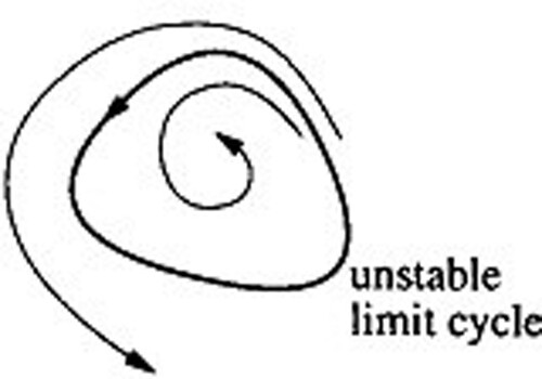
That is constant multiple of $q^7$ and q is also non-zero, $q\ne 0$ taken above. Thus, we conclude that multiplicity of class $C_{10,5}$ is 8, i.e. ${\mu }_{max}\left(C_{10,5}\right)\ge 8.$ As the maximum multiplicity is 8 (even) and is also positive. So, from Remark 3.1, the periodic solutions are unstable (Figure 3).

Figure 3. Stability of Class $C_{10,5}$.

4.2. Trigonometric coefficients for non-homogeneous and homogeneous polynomials

Now, we consider equation of the form as below: (29) $\stackrel{\cdot }{\mathfrak{z}}=\gamma \left(\tau \right){\mathfrak{z}}^3+\delta \left(\tau \right){\mathfrak{z}}^2,$(29) having polynomials $\gamma \left(\tau \right)$ and $\delta \left(\tau \right)$ in $\sin \tau$ and $\cos \tau$; for this we suppose that $\omega =2\pi .$ This brings us closer to Hilbert's sixteenth problem that is original motivation. Equations of the form (29(29) $\stackrel{\cdot }{\mathfrak{z}}=\gamma \left(\tau \right){\mathfrak{z}}^3+\delta \left(\tau \right){\mathfrak{z}}^2,$(29) ) are of Hilbert's type which comes from (1(1) $\stackrel{\cdot }{\mathfrak{z}}=\gamma \left(\tau \right){\mathfrak{z}}^3+\delta \left(\tau \right){\mathfrak{z}}^2+\upsilon \left(\tau \right)\mathfrak{z},$(1) ) with $\upsilon =0,$ γ and δ of degree $2(n+1)$ and $(n+1)$  respectively, are non-homogeneous polynomials. In this context, there are restrictions on the possible values of multiplicity '${\varkappa }^{\mathrm{\prime }}$ which did not apply to the equations considered in Section 4.1; these make problem more complicated. Consider that γ and δ contain only terms of even and odd degree, respectively; same situation is in Hilbert's type with n is even in (1(1) $\stackrel{\cdot }{\mathfrak{z}}=\gamma \left(\tau \right){\mathfrak{z}}^3+\delta \left(\tau \right){\mathfrak{z}}^2+\upsilon \left(\tau \right)\mathfrak{z},$(1) ), for degree of γ and δ. Suppose $\gamma (\pi +\tau )=\gamma \left(\tau \right),$ $\delta (\pi +\tau )=-\delta \left(\tau \right);$ therefore, -$\phi (\tau +\pi )$ is a periodic solution if $\phi \left(\tau \right)$ is such a solution. From the theory of complex analysis, complex solutions always occur in conjugate pairs due to which total number of non-trivial periodic solutions is even. Furthermore, if multiplicity of the origin is odd; for $\varkappa >1$ we can show $(\varkappa -1)$ is even.

In accordance with Section 4.1, we now go off to numerous classes of Equation (29(29) $\stackrel{\cdot }{\mathfrak{z}}=\gamma \left(\tau \right){\mathfrak{z}}^3+\delta \left(\tau \right){\mathfrak{z}}^2,$(29) ). By using computer Algebra Maple18, the calculations in this module are verified. The expressions relating to Theorem 2.2 are of bulk extent that straightforward use of Maple18 integrating operator either failed or progress slow due to insufficient pile space. This difficulty was overcome by individually computing a list of definite integrals of the form ${\int }_0^{2\pi }{\tau }^j{\cos }^m\tau {\sin }^n\tau \mathrm{d}\tau$ using Maple18, firstly we store this in a file and then enter it into an array during a Maple18 run. After this indefinite integrals are calculated for polynomials τ, $sin\tau ,$ and $cos\tau$.

4.2.1. Non-homogeneous trigonometric coefficient

Periodic solutions for the classes $C_{22,11}$ and $C_{24,12}$ are calculated below.

Theorem 4.6

Let the class $C_{22,11}$ for Equation (29(29) $\stackrel{\cdot }{\mathfrak{z}}=\gamma \left(\tau \right){\mathfrak{z}}^3+\delta \left(\tau \right){\mathfrak{z}}^2,$(29) ), if the coefficients are: $\begin{array}{rl}\gamma \left(\tau \right)& =\left(\begin{array}{c}\left(a\right){\sin }^{14}\tau +\left(b\right)\sin \tau {\cos }^{13}\tau \\ +\left(d\right)cos\tau {\sin }^{13}\tau \end{array}\right)\\ & \times {\left({\cos }^2\tau +{\sin }^2\tau \right)}^4,\\ \delta \left(\tau \right)& =\left(\left(g\right)\cos \tau {\sin }^{10}\tau +\left(i\right){\cos }^{10}\tau \sin \tau \right).\end{array}$ Then we calculate ${\varkappa }_{max}\left(C_{22,11}\right)\ge 9.$

Proof.

From Theorem 2.2, we now calculate ${\varkappa }_2=0,$ and $\begin{array}{r}{\varkappa }_3=\frac{429a\pi }{1024}\end{array}$ For ${\varkappa }_3=0,$ by putting value of a = 0,${\varkappa }_4=0$ and by proceeding further we calculate ${\varkappa }_5$ as: $\begin{array}{r}{\varkappa }_5=-\frac{3059gi\pi (b+d)}{47244640256}.\end{array}$ If ${\varkappa }_5=0$ then, either g = i = 0 or: (30) $b+d=0.$(30) If g = i = 0 then $\delta \left(\tau \right)=0,$ and for ${\varkappa }_3=0,$  it shows that mean value of $\gamma \left(\tau \right)$ is zero. As a result, from Corollary 3.2, origin is a centre. From Equation (30(30) $b+d=0.$(30) ), we substitute b = −d and calculate ${\varkappa }_6=0$ with${\varkappa }_7$ as: $\begin{array}{r}{\varkappa }_7=-\frac{2052417dgi\pi (g-i)(g+i)}{68116944363978752}.\end{array}$ For ${\varkappa }_7=0,$ as $\pi gi\ne 0,$ then for d = 0 we get $b=0,$ due to which $\gamma \left(\tau \right)$ is zero for the value of $d=b=a=0,$ and for ${\varkappa }_2=0$ gives that $\delta \left(\tau \right)$ has mean value zero. As a result, origin is a centre from corollary 3.2. So, we take $dgi\pi \ne 0.$ Further, by using the value $g=\pm i,$ we calculate ${\varkappa }_8=0$ and moving in the same manner we calculate ${\varkappa }_9$ as: $\begin{array}{r}{\varkappa }_9=\pm \frac{1539578881388202051}{857233080777916863741952}d{i}^4\pi .\end{array}$ Which is constant multiple of the variables, that are non-zero. Hence ${\mu }_{max}\left(C_{22,11}\right)\ge 9.$

Theorem 4.7

Let the class $C_{24,12}$ for Equation (29(29) $\stackrel{\cdot }{\mathfrak{z}}=\gamma \left(\tau \right){\mathfrak{z}}^3+\delta \left(\tau \right){\mathfrak{z}}^2,$(29) ), if the coefficients are: $\begin{array}{rl}\gamma \left(\tau \right)& =\left(\begin{array}{c}\left(e\right){\sin }^{10}\tau +\left(f\right)\cos \tau {\sin }^9\tau +\\ \left(g\right){\cos }^9\tau \sin \tau +\left(h\right){\cos }^{10}\tau \end{array}\right)\\ & \times {\left({\cos }^2\tau +{\sin }^2\tau \right)}^7,\\ \delta \left(\tau \right)& =\left(\left(a){\cos }^7\tau \sin \tau +\left(b\right){\sin }^7\tau \cos \tau \right)\right)\\ & \times {\left({\cos }^2\tau +{\sin }^2\tau \right)}^2.\end{array}$ Then ${\mu }_{max}\left(C_{24,12}\right)\ge 10$ is presented.

Proof.

With the use of Theorem 2.2, it is easily calculated that ${\varkappa }_2=0$ and: $\begin{array}{r}{\varkappa }_3=\frac{63\pi (e+h)}{128}.\end{array}$ If ${\varkappa }_3=0,$ then, as $\pi \ne 0,$ we substitute value of ”e = −h ” and calculate ${\varkappa }_4$ as: $\begin{array}{r}{\varkappa }_4=-\frac{1515\pi h(a+b)}{32768}.\end{array}$ For ${\varkappa }_4=0,$ if we consider $h\pi \ne 0,$ then we put a = −b, and get ${\varkappa }_5=$ 0 with ${\varkappa }_6$ as: $\begin{array}{r}{\varkappa }_6=-\frac{135387bh\pi (f+g)}{83886080}.\end{array}$ For ${\varkappa }_6=0$, if b = 0 then $a=0,$ and as a result $\delta \left(t\right)=0,$ and for ${\varkappa }_3=0$ shows that mean value of $\gamma \left(\tau \right)$ is zero. As a result, origin is a centre from Corollary 3.2. So, we suppose that $b\ne 0,$ and substitute $f=-g,$ with which we calculate ${\varkappa }_7={\varkappa }_8=0,$ but ${\varkappa }_9$ as: $\begin{array}{r}{\varkappa }_9=\frac{\begin{array}{c}b\pi (94936183603200g^2+235562160127g{b}^3\\ -3396424024719360h^2)\end{array}}{22166154415964160}.\end{array}$ If ${\varkappa }_9=0,$ then as $b\pi \ne 0,$ we put, $\begin{array}{r}{h}^2=\frac{94936183603200}{3396424024719360}{g}^2+\frac{235562160127}{3396424024719360}g{b}^3.\end{array}$ and calculate ${\varkappa }_{10}$ as: $\begin{array}{rl}& {\varkappa }_{10}=\\ & -\frac{\begin{array}{l}{g}^{3}b\pi (7318586589734405455888357785600g{b}^2\\ -173594075291076034335740295905280g^2\\ +9332277799849085034833334665b^5\\ -154578670934888723063647991808g{b}^3.\end{array}}{783162059372457471546426572931072000}\end{array}$ From Theorem 2.2, due to the lack of formula ${\varkappa }_{11},$ which is used to calculate multiplicity greater than 10. So, we cannot move towards further calculations. Hence we conclude that ${\mu }_{max}\left(C_{24,12}\right)\ge 10.$

Finally, for Equation (29(29) $\stackrel{\cdot }{\mathfrak{z}}=\gamma \left(\tau \right){\mathfrak{z}}^3+\delta \left(\tau \right){\mathfrak{z}}^2,$(29) ), we consider homogeneous polynomials with trigonometric coefficients.

4.2.2. Homogeneous trigonometric coefficient

Theorem 4.8

Let $C_{10,10}$ be the class with: $\begin{array}{rl}\gamma \left(\tau \right)& =\left(\begin{array}{c}\left(a\right){\sin }^8\tau +\left(b\right)\cos \tau {\sin }^7\tau +\\ \left(d\right){\cos }^7\tau \sin \tau +\left(e\right){\cos }^8\tau \end{array}\right)\\ & \times \left({\cos }^2\tau +{\sin }^2\tau \right),\\ \delta \left(\tau \right)& =\left(\left(g\right){\cos }^7\tau \sin \tau +\left(h\right)\cos \tau {\sin }^7\tau \right)\\ & \times \left({\cos }^2\tau +{\sin }^2\tau \right).\end{array}$ Then ${\mu }_{max}\left(C_{10,10}\right)\ge 10$ is calculated.

Proof.

With the use of Theorem 2.2, it can be easily calculated that ${\varkappa }_2=0,$ and, $\begin{array}{r}{\varkappa }_3=\frac{35\pi (e+a)}{64}.\end{array}$ For ${\varkappa }_3=0$, by substituting $e=-a,$ we calculate ${\varkappa }_4$ as: $\begin{array}{r}{\varkappa }_4=\frac{25a\pi (g+h)}{512}.\end{array}$ If ${\varkappa }_4=0$ as π is irrational and non-zero, either $a=0,$ or h + g = 0. If a = 0 then $e=0,$ and by substituting $e=a=0,$ γ is the constant multiple of δ and also ${\int }_0^{2\pi }\delta \left(\tau \right)\mathrm{d}t=0.$ Thus from Corollary 3.1, origin is a centre. So, we consider that $a\ne 0,$ and by substituting: (31) $h=-g,$(31) we calculate${\varkappa }_5=0$ and ${\varkappa }_6$ as: $\begin{array}{r}{\varkappa }_6=-\frac{315ga\pi (b+d)}{131072}.\end{array}$ If ${\varkappa }_6=0,$ either $g=0,$ because $a\ne 0$ (considered above) and for g = 0 Equation (31(31) $h=-g,$(31) ) gives h = 0, and as a result $\delta \left(t\right)=0.$ For ${\varkappa }_3=0,$ mean value of $\gamma \left(t\right)$ is zero. So by Corollary 3.2, origin is the centre. Now supposed that $g\ne 0,$  and substituting $d=-b,$ we calculate ${\varkappa }_7=0,$ ${\varkappa }_8=0$ and by proceeding further, ${\varkappa }_9$ is as follows: $\begin{array}{r}{\varkappa }_9=\frac{\begin{array}{l}g\pi (662955045683200000a^2\\ -120365385252864000b^2\\ -39705206001849b{g}^3)\end{array}}{3958241859993600000}.\end{array}$ If ${\varkappa }_9=0,$ as $g\pi \ne 0($shown above), then the substitution of explicit function $a^2$ is as follows: (32) $\begin{array}{rl}{a}^2& =\frac{39705206001849}{662955045683200000}b{g}^3\\ & +\frac{120365385252864000}{662955045683200000}{b}^2.\end{array}$(32) With holding Equation (32(32) $\begin{array}{rl}{a}^2& =\frac{39705206001849}{662955045683200000}b{g}^3\\ & +\frac{120365385252864000}{662955045683200000}{b}^2.\end{array}$(32) ), ${\varkappa }_{10}$ comes out as: $\begin{array}{rl}& {\varkappa }_{10}\\ & =-\frac{\begin{array}{l}{g}^{3}b\pi (130740337229914440440183408640b{g}^3\\ +4717720188035374060782344553g^5\\ +16266549215034938791838613504000b{g}^2\\ +498496355511533840443868446720000b^2)\end{array}}{1492842048351124836385921433600000000}.\end{array}$ From ${\varkappa }_{10}$ we cannot substitute any value for further calculation. Hence we conclude that ${\mu }_{max}\left(C_{10,10}\right)\ge 10.$

5. Conclusion

In this paper, we have obtained some existence results for first-order cubic non-autonomous differential equation by using method of perturbation. A new formula ${\varkappa }_{10}$ is constructed and is used to find maximum multiplicity 10 for various polynomial classes $C_{24,12}$ with non-homogeneous and $C_{10,10}$ with homogeneous trigonometric coefficients, while $C_{10,3}$ and $C_{10,4}$ for polynomial coefficients are presented. We validate our results in accordance with the classical paper by Alwash [12]. This is in fact that solution of Hilbert's Sixteenth problem is still faraway, looking through more limit cycles and escalate the general upper bounds form could be a constructive choice in approaching the problem.

Acknowledgements

The authors would like to express their sincere thanks to the support of National Natural Science Foundation of China. All authors contributed equally to the writing of this paper. All authors read and approved the final manuscript.

Disclosure statement

No potential conflict of interest was reported by the authors.

Additional information

Funding

This work was supported by the National Natural Science Foundation of China [grant number 61673169].

References

- Iqbal M, Seadawy AR, Lu D. Construction of solitary wave solutions to the nonlinear modified Kortewege-de Vries dynamical equation in unmagnetized plasma via mathematical methods. Mod Phys Lett A. 2018;33(32):1850183. doi: 10.1142/S0217732318501833
- Iqbal M, Seadawy AR, Lu D. Dispersive solitary wave solutions of nonlinear further modified Korteweg-de Vries dynamical equation in an unmagnetized dusty plasma. Mod Phys Lett A. 2018;33(37):1850217. doi: 10.1142/S0217732318502176
- Iqbal M, Seadawy AR, Lu D. Applications of nonlinear longitudinal wave equation in a magneto-electro-elastic circular rod and new solitary wave solutions. Mod Phys Lett B. 2019;33(18):1950210. doi: 10.1142/S0217984919502105
- Iqbal M, Seadawy AR, Lu D, et al. Construction of bright–dark solitons and ion-acoustic solitary wave solutions of dynamical system of nonlinear wave propagation. Mod Phys Lett A. 2019;34:1950309.
- Iqbal M, Seadawy AR, Khalil OH, et al. Propagation of long internal waves in density stratified ocean for the (2+1)-dimensional nonlinear Nizhnik-Novikov-Vesselov dynamical equation. Results Phys. 2020;16:102838. doi: 10.1016/j.rinp.2019.102838
- Seadawy AR, Iqbal M, Lu D. Applications of propagation of long-wave with dissipation and dispersion in nonlinear media via solitary wave solutions of generalized Kadomtsev–Petviashvili modified equal width dynamical equation. Comput Math Appl. 2019;78:3620–3632. doi: 10.1016/j.camwa.2019.06.013
- Seadawy AR, Iqbal M, Lu D. The nonlinear diffusion reaction dynamical system with quadratic and cubic nonlinearities with analytical investigations. Int J Mod Phys B. 2020;34(9):2050085. doi: 10.1142/S021797922050085X
- Seadawy AR, Iqbal M, Lu D. Nonlinear wave solutions of the Kudryashov–Sinelshchikov dynamical equation in mixtures liquid-gas bubbles under the consideration of heat transfer and viscosity. J Taibah Univ Sci. 2019;13(1):1060–1072. doi: 10.1080/16583655.2019.1680170
- Seadawy AR, Iqbal M, Lu D. Propagation of kink and anti-kink wave solitons for the nonlinear damped modified Korteweg–de Vries equation arising in ion-acoustic wave in an unmagnetized collisional dusty plasma. Stat Mech Appl. 2020;544:123560.
- Seadawy AR, Iqbal M, Baleanu D. Construction of traveling and solitary wave solutions for wave propagation in nonlinear low-pass electrical transmission lines. J King Saud Univ – Sci. 2020. https://doi.org/10.1016/j.jksus.2020.06.011
- Seadawy AR, Iqbal M, lu D. Construction of soliton solutions of the modify unstable nonlinear schrödinger dynamical equation in fiber optics. Indian J Phys. 2020;94:823–832. doi: 10.1007/s12648-019-01532-5
- Al-Wash MAM, Llyod NG. Non-autonomous equation related to polynomial two-dimensional system. Proc Royal Soc Edinb A. 1987;105:129–152. doi: 10.1017/S0308210500021971
- Alwash MAM. Periodic solutions of polynomial non-autonomous differential equations. Electron J Differ Equ. 2005;84:1–8.
- Yasmin N, Ashraf M. Bifurcating periodic solutions of class C2,4 and C4,3 of research. Sci BZU. 2003;14:225–234.
- Lins Neto A. On the number of solutions of the equations dxdτ=∑j=0naj(τ)τ′,0≤τ≤1 for which x(0)=x(1). Invent Math. 1980;59:67–76. doi: 10.1007/BF01390315
- Llyod NG. The number of periodic solutions of the equation z⋅=p0(τ)zn+p1(τ)zn−1+P2(τ)zn−2+⋯+Pn(τ). Proc London Math Soc. 1973;27:667–700. doi: 10.1112/plms/s3-27.4.667
- Llyod NG. Limit cycles of certain polynomial systems. In: Singh SP, editor. Non-linear functional analysis and its applications (NATO ASI Series; Vol. 173). Dordrecht: Springer; 1986. p. 317–326.
- Hilbert D. Mathematical problems. Bull Amer Math Soc. 1902;8:437–480. doi: 10.1090/S0002-9904-1902-00923-3
- Alwash MAM. Polynomial differential equations with small coefficients. Discrete Contin Dyn Syst. 2009;25:1129–1141. doi: 10.3934/dcds.2009.25.1129
- Bibikov YN, Bukaty VR. Bifurcation of an oscillatory mode under a periodic perturbation of a special oscillator. Differ Equ. 2019;55:753–757. doi: 10.1134/S001226611906003X
- Yasmin N. Closed orbits of certain two dimensional cubic systems [PhD thesis]. Aberystwyth, Wlaes: U. C. W Aberystwyth; 1989. p. 1–134.
- Nawaz A. Bifurcation of periodic solutions of certain classes of cubic non-autonomous differential equations [M.Phil thesis]. Islamabad, Pakistan; 2018. p. 1–104.
- Yasmin N. Bifurcating periodic solutions of polynomial system. Punjab Univ J Math. 2001;34:43–64.
- Akram S, Nawaz A, Yasmin N, et al. Periodic solutions of some classes of one dimensional non-autonomous system. Front Phys. http://doi.org/10.3389/fphy.2020.002642020