On bounds for topological descriptors of φ-sum graphs

Abstract

The properties of chemical compounds are very important for the studies of the non-isomorphism phenomenon's related to the molecular graphs. Topological indices (TIs) are one of the mathematical tools which are used to study these properties. Gutman and Trinajsti [Graph theory and molecular orbitals. Total π-electron energy of alternant hydrocarbons. Chem Phys Lett. 1972;17(4):535–538] defined the Zagreb indices (descriptors) to find correlation value between a molecular graph and its total π-electron energy. Later on, Bollobás and Erdös [Graphs of extremal weights. Ars Comb; 1998;50:225–233] defined the most general form of these indices (descriptors) called by general Randić index (GRI) and first general Zagreb index (FGZI), respectively. In this paper, we computed the bounds for FGZI and GRI of φ-sum graphs, obtained by the strong product of the graph $\phi \left(G\right)$ with another graph Γ, where $\phi \left(G\right)$ is constructed using four subdivision operations on the graph G. At the end, we also include the results for some particular families of graphs as the applications of the obtained results.

Keywords:

• Topological descriptors
• φ-sum graphs
• strong product

MSC (2020) Subject Classifications:

• 05C09
• 05C92

1. Introduction

A number, polynomial or a matrix can uniquely identify a graph and a topological index (TI) of a molecular graph is a numeric number that can be defined as a function $\mathbb{F}:a\mathbb{C}a⟶a\mathbb{R}$, where $\mathbb{C}$ is a class of molecular graphs and $\mathbb{R}$ is a set of real numbers. TI's are classified into different classes but degree-based are most familiar, see [1]. These are used to characterize the physicochemical properties of chemical compounds of the molecular graphs like surface tension $\mathrm{\&}$ density, melting $\mathrm{\&}$ freezing point, heat of evaporation $\mathrm{\&}$ formation and solubility, see [2–4]. TI's are also used in the studies of the structural properties of computer-based networks such as clustering, connectivity, modularity, robustness and vulnerability, see [5].

In computational graph theory, the concept of formation of the new graphs by using some operations is studied widely. For a connected molecular graph G, Yan et al. [6] defined the new graphs called as line graph $L\left(G\right)$, subdivided graph $S\left(G\right)$, triangle parallel graph $R\left(G\right)$, line superposition graph $Q\left(G\right)$ and total graph $T\left(G\right)$ using the subdivision related operations L, S, R, Q and T on G, respectively. They also obtained the Wiener index of these new resultant graphs $\phi \left(G\right)$, where $\phi \in \{L,S,R,Q,T\}$. Eliasi et al. [7] defined the φ-sum graphs $\left(G_{\phi }\mathrm{\Gamma }\right)$ using the operation of cartesian product on the graphs $\phi \left(G\right)$ and Γ. They also obtained the Wiener index of these φ-sum graphs $G_S\mathrm{\Gamma }$, $G_R\mathrm{\Gamma }$, $G_Q\mathrm{\Gamma }$ and $G_T\mathrm{\Gamma }$. The first, second and forgotten zagreb indices of the φ-sum graphs are computed in [8,9]. The first general Zagreb index and general sum-connectivity index of the aforesaid cartesian product-based φ-sum graphs are obtained in the form of exact formulas and bounds, see [10–12]. For further studies of the TIs on the graphs obtained by the various operations of graphs, we refer to [13–21].

Recently, Sarala et al. [22] obtained the F-index of the strong product based φ-sum graphs. The theme of this note is to compute FGZI and GRI of φ-sum graphs $G_{+\phi }\mathrm{\Gamma }$ constructed by the strong product of graphs $\phi \left(G\right)$ and Γ, where $\phi \left(G\right)\in \left\{\right(S\left(G\right),R\left(G\right),Q\left(G\right),T\left(G\right)\}$. The remaining paper is organized as: Section 2 contains some basic definitions and operations on graphs G and $\phi \left(G\right)$, Section 3 covers the main results of upper and lower bounds of FGZI and GRI and Section 4 is devoted to conclusion.

2. Preliminaries

Let G = $\left(V\right(G)$, $E\left(G\right))$ be an undirected, simple, finite and connected molecular graph with vertex set $V\left(G\right)$ and edge set $E\left(G\right)$ such that each vertex presents atom and each edge shows the bonding among the atoms. Degree of u in G is ${\mathrm{\Omega }}_G\left(u\right)=|\{x\in V(G):d(x,u)=1\}|$. The maximum and minimum degrees of a graph G are defined as ${△}_G=\mathrm{m}\mathrm{a}\mathrm{x}\left\{{\mathrm{\Omega }}_G\right(u):\mathrm{\forall }\phantom{a}u\in V(G\left)\right\}$ and ${\delta }_G=\mathrm{m}\mathrm{i}\mathrm{n}\left\{{\mathrm{\Omega }}_G\right(u):\mathrm{\forall }\phantom{a}u\in V(G\left)\right\}$. We note that ${\delta }_G\le {\mathrm{\Omega }}_G\left(u\right)\le {△}_G$, where equality holds if and only if G is a regular graph. For further study of graph-theocratic terminologies, see [23–25]. Now, we define some important degree-based TIs.

Definition 2.1

For a molecular graph G, the first and second Zagreb indices (descriptors) are defined as: $\begin{array}{rl}{M}_1\left(G\right)& =\sum _{vϵV\left(G\right)}\left[{\mathrm{\Omega }}_G\right(v){]}^2\\ & =\sum _{uvϵE\left(G\right)}\left[{\mathrm{\Omega }}_G\right(v)+{\mathrm{\Omega }}_G(u\left)\right]\mathrm{a}\mathrm{n}\mathrm{d}\\ M_2\left(G\right)& =\sum _{uvϵE\left(G\right)}\left[{\mathrm{\Omega }}_G\right(v\left){\mathrm{\Omega }}_G\right(u\left)\right].\end{array}$ In 1972, Gutman and Trinajsti defined these indices (descriptors) to study the molecular graphs, see [26–28].

Definition 2.2

[29,30]

First general Zagreb (FGZ) and general Randi$\acute{c}$ (GR) indices of a molecular graph G are $\begin{array}{rl}{M}_1^{\alpha }& =\sum _{vϵV\left(G\right)}{\mathrm{\Omega }}_G^{\alpha }\left(v\right)\\ & =\sum _{uvϵE\left(G\right)}\left[{\mathrm{\Omega }}_G^{\alpha -1}\right(u)+{\mathrm{\Omega }}_G^{\alpha -1}(v\left)\right]\mathrm{a}\mathrm{n}\mathrm{d}\\ R^{\text{β}}\left(G\right)& =\sum _{uvϵE\left(G\right)}\left[{\mathrm{\Omega }}_G\right(u\left){\mathrm{\Omega }}_G\right(v){]}^{\text{β}}\end{array}$ respectively, where $\alpha \notin \{0,1\}$ and β are real numbers. Moreover, for $\alpha =2$ and $\alpha =3$, FGZI becomes first Zagreb index and forgotten topological index. Similarly, for $\text{β}=1$ and $\text{β}=-\frac{1}{2}$, GRI becomes second Zagreb index and classical Randić index respectively, see [26–32].

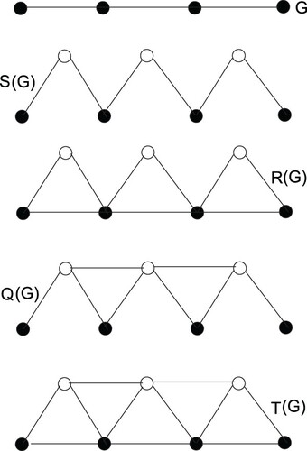
Operations of Subdivision: The following operations are defined in [7].

• $S\left(G\right)$ is obtained by adding a new vertex in each edge of G.

• To obtain $R\left(G\right)$, in $S\left(G\right)$ join end (original) vertices of the edges which are incident on each new vertex.

• To obtain $Q\left(G\right)$, in $S\left(G\right)$ join those pairs of new vertices by edges which have common adjacent (original) vertices.

• If both $R\left(G\right)$ and $Q\left(G\right)$ are applied at the same on $S\left(G\right)$, we obtain $T\left(G\right)$.

Figure 1 illustrates the foresaid operations of the subdivision of graphs.

Figure 1. Subdivision-related operations.

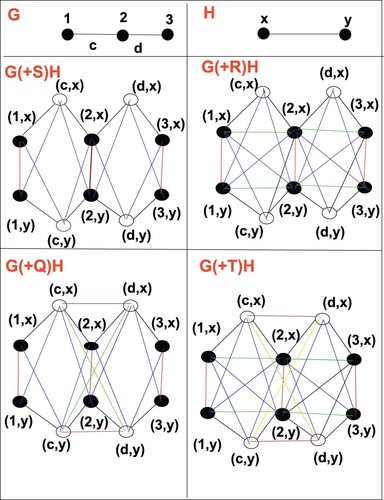
Definition 2.3

For $\phi \in \{S,R,Q,T\}$, $\phi \left(G\right)$ is a graph obtained by the operation φ on graph G with the vertices $V\left(\phi \right(G\left)\right)$ and the edges $E\left(\phi \right(G\left)\right)$. Then, φ-sum graph $G_{+\phi }\mathrm{\Gamma }$ based on strong product of graphs $\phi \left(G\right)$ and Γ is a graph with vertex set $V\left(G_{+\phi }\mathrm{\Gamma }\right)=V\left(\phi \right(G\left)\right)\times V\left(\mathrm{\Gamma }\right)=(V_1\cup E_1)\times \left(V_2\right)$ such that two vertices $(u_1,v_1)$ and $(u_2,v_2)$ of $V\left(G_{+\phi }\mathrm{\Gamma }\right)$ are adjacent iff, either [$u_1=u_2$ ε $V\left(G\right)$ and $v_1{v}_2$ ε $E\left(\mathrm{\Gamma }\right)$] or [$v_1=v_2$ ε $V\left(\mathrm{\Gamma }\right)$ and $u_1{u}_2$ ε $E\left(\phi \right(G\left)\right)$] or [$u_1{u}_2$ ε $E\left(\phi \right(G\left)\right)$ and $v_1{v}_2$ ε $E\left(\mathrm{\Gamma }\right)$], see Figure 2.

Figure 2. The φ-sum graphs for $G=P_3$ and $H=P_2$.

Remark 2.4

For any vertex $(u,v)\in V\left(G_{+\phi }\mathrm{\Gamma }\right)$, the degree of $(u,v)$ (denoted by $d(u,v)$) can be defined as $d(u,v)=\left\{\begin{array}{l}{\mathrm{\Omega }}_{\phi \left(G\right)}\left(u\right)+{\mathrm{\Omega }}_{\mathrm{\Gamma }}\left(v\right)+{\mathrm{\Omega }}_{\phi \left(G\right)}\left(u\right){\mathrm{\Omega }}_{\mathrm{\Gamma }}\left(v\right)\\ \mathrm{i}\mathrm{f}uϵV\left(G\right)\\ {\mathrm{\Omega }}_{\phi \left(G\right)}\left(u\right)+{\mathrm{\Omega }}_{\phi \left(G\right)}\left(u\right){\mathrm{\Omega }}_{\mathrm{\Gamma }}\left(v\right)\\ \mathrm{i}\mathrm{f}uϵV\left(\phi \right(G\left)\right)-V\left(G\right).\end{array}\right.$

3. Main results

This section contains the main results of φ-sum graphs based on strong product. Assume that the connected graphs G and Γ have number of vertices $n_G$ and $n_{\mathrm{\Gamma }}$, and number of edges $m_G$ and $m_{\mathrm{\Gamma }}$, respectively.

Theorem 3.1

Let G and Γ be two connected graph.

1. We have ${\alpha }_2\le M^{\alpha }\left(G_{+s}\mathrm{\Gamma }\right)\le {\alpha }_1,$ where ${\alpha }_1,$ ${\alpha }_2$ $\ge 0$ and $\begin{array}{rl}{\alpha }_1& =2[{△}_G+{△}_{\mathrm{\Gamma }}+{△}_G{△}_{\mathrm{\Gamma }}{]}^{\alpha -1}\\ & \times [n_G{m}_{\mathrm{\Gamma }}+m_G(n_{\mathrm{\Gamma }}+m_{\mathrm{\Gamma }}\left)\right]\\ & +2m_G[{△}_G+{△}_G{△}_{\mathrm{\Gamma }}{]}^{\alpha -1}[m_{\mathrm{\Gamma }}+n_{\mathrm{\Gamma }}]\\ {\alpha }_2& =2[{\delta }_G+{\delta }_{\mathrm{\Gamma }}+{\delta }_G{\delta }_{\mathrm{\Gamma }}{]}^{\alpha -1}\\ & \times [n_G{m}_{\mathrm{\Gamma }}+m_G(n_{\mathrm{\Gamma }}+m_{\mathrm{\Gamma }}\left)\right]\\ & +2m_G[{\delta }_G+{\delta }_G{\delta }_{\mathrm{\Gamma }}{]}^{\alpha -1}[m_{\mathrm{\Gamma }}+n_{\mathrm{\Gamma }}].\end{array}$

2. We have ${\text{β}}_2\le R^{\text{β}}\left(G_{+s}\mathrm{\Gamma }\right)\le {\text{β}}_1,$ where ${\text{β}}_1,$ ${\text{β}}_2$ $\ge 0$ and $\begin{array}{rl}{\text{β}}_1& =n_G{m}_{\mathrm{\Gamma }}[{△}_G+{△}_{\mathrm{\Gamma }}+{△}_G{△}_{\mathrm{\Gamma }}{]}^{2\text{β}}\\ & +2m_G[{△}_G+{△}_{\mathrm{\Gamma }}+{△}_G{△}_{\mathrm{\Gamma }}{]}^{\text{β}}[{△}_G+{△}_G{△}_{\mathrm{\Gamma }}{]}^{\text{β}}\\ & \times [n_{\mathrm{\Gamma }}+m_{\mathrm{\Gamma }}]\\ {\text{β}}_2& =n_G{m}_{\mathrm{\Gamma }}[{\delta }_G+{\delta }_{\mathrm{\Gamma }}+{\delta }_G{\delta }_{\mathrm{\Gamma }}{]}^{2\text{β}}\\ & +2m_G[{\delta }_G+{\delta }_{\mathrm{\Gamma }}+{\delta }_G{\delta }_{\mathrm{\Gamma }}{]}^{\text{β}}[{\delta }_G+{\delta }_G{\delta }_{\mathrm{\Gamma }}{]}^{\text{β}}\\ & \times [n_{\mathrm{\Gamma }}+m_{\mathrm{\Gamma }}].\end{array}$

Proof.

By definition $\left(a\right)M^{\alpha }\left(G_{+s}\mathrm{\Gamma }\right)=\sum _{(u,v)ϵV\left(G_{+s}\mathrm{\Gamma }\right)}{d}_{G_{+s}\mathrm{\Gamma }}^{\alpha }(u,v)$ In terms of edges, where $n=\alpha -1$ $\begin{array}{rl}{M}^{\alpha }\left(G_{+s}\mathrm{\Gamma }\right)& =\sum _{(s_1,t_1)(s_2,t_2)ϵE\left(G_{+s}\mathrm{\Gamma }\right)}\left[d_{G_{+s}\mathrm{\Gamma }}^n\right(s_1,t_1)\\ & +d_{G_{+s}\mathrm{\Gamma }}^n(s_2,t_2)]\\ & =\sum _{s_1=s_2ϵV\left(G\right)}\sum _{\left(t_1{t}_2\right)ϵE\left(\mathrm{\Gamma }\right)}\left[d_{G_{+s}\mathrm{\Gamma }}^n\right(s_1,t_1)\\ & +d_{G_{+s}\mathrm{\Gamma }}^n(s_2,t_2)]\\ & +\sum _{t_1=t_2ϵV\left(\mathrm{\Gamma }\right)}\sum _{\left(s_1{s}_2\right)ϵE\left(S\right(G\left)\right)}\left[d_{G_{+s}\mathrm{\Gamma }}^n\right(s_1,t_1)\\ & +d_{G_{+s}\mathrm{\Gamma }}^n(s_2,t_2)]\\ & +\sum _{s_1{s}_2ϵE\left(S\right(G\left)\right)}\sum _{\left(t_1{t}_2\right)ϵE\left(\mathrm{\Gamma }\right)}\left[d_{G_{+s}\mathrm{\Gamma }}^n\right(s_1,t_1)\\ & +d_{G_{+s}\mathrm{\Gamma }}^n(s_2,t_2)]\\ & =\sum _1+\sum _2+\sum _3.\end{array}$ Consider, $\begin{array}{rl}\sum _1& =\sum _{s_1=s_2ϵV\left(G\right)}\sum _{\left(t_1{t}_2\right)ϵE\left(\mathrm{\Gamma }\right)}\left[d_{G_{+s}\mathrm{\Gamma }}^n\right(s_1,t_1)+d_{G_{+s}\mathrm{\Gamma }}^n(s_2,t_2\left)\right]\\ & =\sum _{s_1=s_2ϵV\left(G\right)}\sum _{\left(t_1{t}_2\right)ϵE\left(\mathrm{\Gamma }\right)}\left[\right\{{\mathrm{\Omega }}_{\left(G\right)}{s}_1+{\mathrm{\Omega }}_{\left(\mathrm{\Gamma }\right)}{t}_1\\ & +{\mathrm{\Omega }}_{\left(G\right)}{s}_1{\mathrm{\Omega }}_{\left(\mathrm{\Gamma }\right)}{t}_1{\}}^n+\{{\mathrm{\Omega }}_{\left(G\right)}{s}_2+{\mathrm{\Omega }}_{\left(\mathrm{\Gamma }\right)}{t}_2\\ & +{\mathrm{\Omega }}_{\left(G\right)}{s}_2{\mathrm{\Omega }}_{\left(\mathrm{\Gamma }\right)}{t}_2{\}}^n]\\ & \le \sum _{s_1=s_2ϵV\left(G\right)}\sum _{\left(t_1{t}_2\right)ϵE\left(\mathrm{\Gamma }\right)}\left[\right\{{△}_G+{△}_{\mathrm{\Gamma }}+{△}_G{△}_{\mathrm{\Gamma }}{\}}^n\\ & +\{{△}_G+{△}_{\mathrm{\Gamma }}+{△}_G{△}_{\mathrm{\Gamma }}{\}}^n]\\ & =2n_G{m}_{\mathrm{\Gamma }}\{{△}_G+{△}_{\mathrm{\Gamma }}+{△}_G{△}_{\mathrm{\Gamma }}{\}}^n.\end{array}$ It is clear that ${△}_{S\left(G\right)}$ = ${△}_G$ and $\mid E\left(S\right(G\left)\right)\mid$ = $2\mid E\left(G\right)\mid$. Therefore ∀$\{t_1=t_2\}$ε $V\left(\mathrm{\Gamma }\right)$ $\mathrm{\&}$ $\left\{s_1{s}_2\right\}$ ε $E\left(S\right(G\left)\right)$ with $s_1$ ε $V\left(G\right)$, $s_2$ ε $\left(V\right(S\left(G\right))-V(G\left)\right)$ we have $\begin{array}{rl}\sum _2& =\sum _{t_1=t_2ϵV\left(\mathrm{\Gamma }\right)}\sum _{\left(s_1{s}_2\right)ϵE\left(S\right(G\left)\right)}\left[d_{G_{+s}\mathrm{\Gamma }}^n\right(s_1,t_1)\\ & +d_{G_{+s}\mathrm{\Gamma }}^n(s_2,t_2)]\\ & =\sum _{t_1=t_2ϵV\left(\mathrm{\Gamma }\right)}\sum _{\left(s_1{s}_2\right)ϵE\left(S\right(G\left)\right)}\left[\right\{{\mathrm{\Omega }}_{\left(G\right)}{s}_1+{\mathrm{\Omega }}_{\left(\mathrm{\Gamma }\right)}{t}_1\\ & +{\mathrm{\Omega }}_{\left(G\right)}{s}_1{\mathrm{\Omega }}_{\left(\mathrm{\Gamma }\right)}{t}_1{\}}^n+\{{\mathrm{\Omega }}_{\left(G\right)}{s}_2+{\mathrm{\Omega }}_{\left(G\right)}{s}_2{\mathrm{\Omega }}_{\left(\mathrm{\Gamma }\right)}{t}_2{\}}^n]\\ & \le \sum _{t_1=t_2ϵV\left(\mathrm{\Gamma }\right)}\sum _{\left(s_1{s}_2\right)ϵE\left(S\right(G\left)\right)}\left[\right\{{△}_G(1+{△}_{\mathrm{\Gamma }})+{△}_{\mathrm{\Gamma }}{\}}^n\\ & +\left\{{△}_G\right(1+{△}_{\mathrm{\Gamma }}\left){\}}^n\right]\\ & =2n_{\mathrm{\Gamma }}{m}_G\left[\right\{{△}_G(1+{△}_{\mathrm{\Gamma }})+{△}_{\mathrm{\Gamma }}{\}}^n+\left\{{△}_G\right(1+{△}_{\mathrm{\Gamma }}\left){\}}^n\right].\end{array}$ Now ∀$s_1{s}_2$ε $E\left(S\right(G\left)\right)$ such that $s_1ϵE\left(G\right)$ $\mathrm{\&}$ $s_2$ ε $\left(V\right(S\left(G\right))-V(G\left)\right)$ and $\left(t_1{t}_2\right)$ ε $E\left(\mathrm{\Gamma }\right)$, we have $\begin{array}{rl}\sum _3& =\sum _{s_1{s}_2ϵE\left(S\right(G\left)\right)}\sum _{\left(t_1{t}_2\right)ϵE\left(\mathrm{\Gamma }\right)}\left[d_{G_{+s}\mathrm{\Gamma }}^n\right(s_1,t_1)+d_{G_{+s}\mathrm{\Gamma }}^n(s_2,t_2\left)\right]\\ & =\sum _{s_1{s}_2ϵE\left(S\right(G\left)\right)}\sum _{\left(t_1{t}_2\right)ϵE\left(\mathrm{\Gamma }\right)}\left[\right\{{\mathrm{\Omega }}_{\left(G\right)}{s}_1+{\mathrm{\Omega }}_{\left(\mathrm{\Gamma }\right)}{t}_1\\ & +{\mathrm{\Omega }}_{\left(G\right)}{s}_1{\mathrm{\Omega }}_{\left(\mathrm{\Gamma }\right)}{t}_1{\}}^n+\{{\mathrm{\Omega }}_{\left(G\right)}{s}_2+{\mathrm{\Omega }}_{\left(G\right)}{s}_2{\mathrm{\Omega }}_{\left(\mathrm{\Gamma }\right)}{t}_2{\}}^n]\\ & \le \sum _{\left(\genfrac{}{}{0em}{}{s_1ϵV\left(G\right),s_2}{ϵV\left(S\right(G\left)\right)-V\left(G\right)}\right)}\sum _{\left(t_1{t}_2\right)ϵE\left(\mathrm{\Gamma }\right)}\left[\right\{{△}_G+{△}_{\mathrm{\Gamma }}+{△}_G{△}_{\mathrm{\Gamma }}{\}}^n\\ & +\{{△}_G+{△}_G{△}_{\mathrm{\Gamma }}{\}}^n]\\ & =m_{\mathrm{\Gamma }}|E\left(S\right(G\left)\right)|\left[\right\{{△}_G+{△}_{\mathrm{\Gamma }}+{△}_G{△}_{\mathrm{\Gamma }}{\}}^n\\ & +\{{△}_G+{△}_G{△}_{\mathrm{\Gamma }}{\}}^n]\\ & =2m_G{m}_{\mathrm{\Gamma }}\left[\right\{{△}_G+{△}_{\mathrm{\Gamma }}+{△}_G{△}_{\mathrm{\Gamma }}{\}}^n\\ & +\{{△}_G+{△}_G{△}_{\mathrm{\Gamma }}{\}}^n].\end{array}$ Consequently, $\begin{array}{rl}{M}^{\alpha }\left(G_{+s}\mathrm{\Gamma }\right)& \le 2[{△}_G+{△}_{\mathrm{\Gamma }}+{△}_G{△}_{\mathrm{\Gamma }}{]}^{\alpha -1}\\ & \times [n_G{m}_{\mathrm{\Gamma }}+m_G(n_{\mathrm{\Gamma }}+m_{\mathrm{\Gamma }}\left)\right]\\ & +2m_G[{△}_G+{△}_G{△}_{\mathrm{\Gamma }}{]}^{\alpha -1}[m_{\mathrm{\Gamma }}+n_{\mathrm{\Gamma }}].\end{array}$ Similarly, we can compute $\begin{array}{rl}{M}^{\alpha }\left(G_{+s}\mathrm{\Gamma }\right)& \ge 2[{\delta }_G+{\delta }_{\mathrm{\Gamma }}+{\delta }_G{\delta }_{\mathrm{\Gamma }}{]}^{\alpha -1}\\ & \times [n_G{m}_{\mathrm{\Gamma }}+m_G(n_{\mathrm{\Gamma }}+m_{\mathrm{\Gamma }}\left)\right]\\ & +2m_G[{\delta }_G+{\delta }_G{\delta }_{\mathrm{\Gamma }}{]}^{\alpha -1}[m_{\mathrm{\Gamma }}+n_{\mathrm{\Gamma }}].\end{array}$ equality holds iff G and Γ are regular graphs. $\begin{array}{rl}\left(b\right)& R^{\text{β}}\left(G_{+s}\mathrm{\Gamma }\right)\\ & =\sum _{(s_1,t_1)(s_2,t_2)ϵE\left(G+s\mathrm{\Gamma }\right)}\left[{\mathrm{\Omega }}_{G_{+s}\mathrm{\Gamma }}\right(s_1,t_1)\\ & \times {\mathrm{\Omega }}_{G_{+s}\mathrm{\Gamma }}(s_2,t_2){]}^{\text{β}}\\ & =\sum _{s_1=s_2ϵV\left(G\right)}\sum _{\left(t_1{t}_2\right)ϵE\left(\mathrm{\Gamma }\right)}\left[{\mathrm{\Omega }}_{G_{+s}\mathrm{\Gamma }}\right(s_1,t_1)\\ & \times {\mathrm{\Omega }}_{G_{+s}\mathrm{\Gamma }}(s_2,t_2){]}^{\text{β}}\\ & +\sum _{t_1=t_2ϵV\left(\mathrm{\Gamma }\right)}\sum _{\left(s_1{s}_2\right)ϵE\left(S\right(G\left)\right)}\left[{\mathrm{\Omega }}_{G_{+s}\mathrm{\Gamma }}\right(s_1,t_1)\\ & \times {\mathrm{\Omega }}_{G_{+s}\mathrm{\Gamma }}(s_2,t_2){]}^{\text{β}}\\ & +\sum _{s_1{s}_2ϵE\left(S\right(G\left)\right)}\sum _{\left(t_1{t}_2\right)ϵE\left(\mathrm{\Gamma }\right))}\left[{\mathrm{\Omega }}_{G_{+s}\mathrm{\Gamma }}\right(s_1,t_1)\\ & \times {\mathrm{\Omega }}_{G_{+s}\mathrm{\Gamma }}(s_2,t_2){]}^{\text{β}}\\ & =\sum _1+\sum _2+\sum _3.\end{array}$ Consider, $\begin{array}{rl}\sum _1& =\sum _{s_1=s_2ϵV\left(G\right)}\sum _{\left(t_1{t}_2\right)ϵE\left(\mathrm{\Gamma }\right)}\left[{\mathrm{\Omega }}_{G_{+s}\mathrm{\Gamma }}\right(s_1,t_1)\\ & \times {\mathrm{\Omega }}_{G_{+s}\mathrm{\Gamma }}(s_2,t_2){]}^{\text{β}}\\ & =\sum _{s_1=s_2ϵV\left(G\right)}\sum _{\left(t_1{t}_2\right)ϵE\left(\mathrm{\Gamma }\right)}\left[\right({\mathrm{\Omega }}_{S\left(G\right)}{s}_1+{\mathrm{\Omega }}_{\left(\mathrm{\Gamma }\right)}{t}_1\\ & +{\mathrm{\Omega }}_{S\left(G\right)}{s}_1{\mathrm{\Omega }}_{\left(\mathrm{\Gamma }\right)}{t}_1)\\ & \times ({\mathrm{\Omega }}_{S\left(G\right)}{s}_2+{\mathrm{\Omega }}_{\left(\mathrm{\Gamma }\right)}{t}_2+{\mathrm{\Omega }}_{S(G}{s}_2{\mathrm{\Omega }}_{\left(\mathrm{\Gamma }\right)}{t}_2){]}^{\text{β}}\\ & \le \sum _{s_1=s_2ϵV\left(G\right)}\sum _{\left(t_1{t}_2\right)ϵE\left(\mathrm{\Gamma }\right)}[{△}_G+{△}_{\mathrm{\Gamma }}+{△}_G{△}_{\mathrm{\Gamma }}{]}^{2\text{β}}\\ & =n_G{m}_{\mathrm{\Gamma }}[{△}_G+{△}_{\mathrm{\Gamma }}+{△}_G{△}_{\mathrm{\Gamma }}{]}^{2\text{β}}.\\ \sum _2& =\sum _{t_1=t_2ϵV\left(\mathrm{\Gamma }\right)}\sum _{\left(s_1{s}_2\right)ϵE\left(S\right(G\left)\right)}\left[{\mathrm{\Omega }}_{G_{+s}\mathrm{\Gamma }}\right(s_1,t_1)\\ & \times {\mathrm{\Omega }}_{G_{+s}\mathrm{\Gamma }}(s_2,t_2){]}^{\text{β}}\\ & =\sum _{t_1=t_2ϵV\left(\mathrm{\Gamma }\right)}\sum _{\left(s_1{s}_2\right)ϵE\left(S\right(G\left)\right)}\left[\right({\mathrm{\Omega }}_{S\left(G\right)}{s}_1+{\mathrm{\Omega }}_{\left(\mathrm{\Gamma }\right)}{t}_1\\ & +{\mathrm{\Omega }}_{S\left(G\right)}{s}_1{\mathrm{\Omega }}_{\left(\mathrm{\Gamma }\right)}{t}_1)\\ & \times ({\mathrm{\Omega }}_{S\left(G\right)}{s}_2+{\mathrm{\Omega }}_{S\left(G\right)}{s}_2{\mathrm{\Omega }}_{\left(\mathrm{\Gamma }\right)}{t}_2){]}^{\text{β}}\\ & \le 2n_{\mathrm{\Gamma }}{m}_G\left[\right({△}_G+{△}_{\mathrm{\Gamma }}+{△}_G{△}_{\mathrm{\Gamma }}\left)\right({△}_G+{△}_G{△}_{\mathrm{\Gamma }}){]}^{\text{β}}.\\ \sum _3& =\sum _{s_1{s}_2ϵE\left(S\right(G\left)\right)}\sum _{\left(t_1{t}_2\right)ϵE\left(\mathrm{\Gamma }\right)}\left[{\mathrm{\Omega }}_{G_{+s}\mathrm{\Gamma }}\right(s_1,t_1)\\ & \times {\mathrm{\Omega }}_{G_{+s}\mathrm{\Gamma }}(s_2,t_2){]}^{\text{β}}\\ & =\sum _{s_1ϵV\left(G\right),s_2ϵV\left(S\right(G\left)\right)-V\left(G\right)}\sum _{\left(t_1{t}_2\right)ϵE\left(\mathrm{\Gamma }\right)}\left[\right({\mathrm{\Omega }}_{S\left(G\right)}{s}_1+{\mathrm{\Omega }}_{\left(\mathrm{\Gamma }\right)}{t}_1\\ & +{\mathrm{\Omega }}_{S\left(G\right)}{s}_1{\mathrm{\Omega }}_{\left(\mathrm{\Gamma }\right)}{t}_1)\\ & \times ({\mathrm{\Omega }}_{S\left(G\right)}{s}_2+{\mathrm{\Omega }}_{S\left(G\right)}{s}_2{\mathrm{\Omega }}_{\left(\mathrm{\Gamma }\right)}{t}_2){]}^{\text{β}}\\ & \le m_{\mathrm{\Gamma }}|E\left(S\right(G\left)\right)|\left[\right({△}_G+{△}_{\mathrm{\Gamma }}+{△}_G{△}_{\mathrm{\Gamma }})\\ & \times ({△}_G+{△}_G{△}_{\mathrm{\Gamma }}){]}^{\text{β}}\\ & =2m_G{m}_{\mathrm{\Gamma }}\left[\right({△}_G+{△}_{\mathrm{\Gamma }}+{△}_G{△}_{\mathrm{\Gamma }}\left)\right({△}_G+{△}_G{△}_{\mathrm{\Gamma }}){]}^{\text{β}}.\end{array}$ Therefore, $\begin{array}{rl}{R}^{\text{β}}\left(G_{+s}\mathrm{\Gamma }\right)& \le n_G{m}_{\mathrm{\Gamma }}[{△}_G+{△}_{\mathrm{\Gamma }}+{△}_G{△}_{\mathrm{\Gamma }}{]}^{2\text{β}}\\ & +2m_G[{△}_G+{△}_{\mathrm{\Gamma }}+{△}_G{△}_{\mathrm{\Gamma }}{]}^{\text{β}}\\ & \times [{△}_G+{△}_G{△}_{\mathrm{\Gamma }}{]}^{\text{β}}[n_{\mathrm{\Gamma }}+m_{\mathrm{\Gamma }}].\end{array}$ Similarly, we can compute $\begin{array}{rl}{R}^{\text{β}}\left(G_{+s}\mathrm{\Gamma }\right)& \ge n_G{m}_{\mathrm{\Gamma }}[{\delta }_G+{\delta }_{\mathrm{\Gamma }}+{\delta }_G{\delta }_{\mathrm{\Gamma }}{]}^{2\text{β}}\\ & +2m_G[{\delta }_G+{\delta }_{\mathrm{\Gamma }}+{\delta }_G{\delta }_{\mathrm{\Gamma }}{]}^{\text{β}}\\ & \times [{\delta }_G+{\delta }_G{\delta }_{\mathrm{\Gamma }}{]}^{\text{β}}[n_{\mathrm{\Gamma }}+m_{\mathrm{\Gamma }}].\end{array}$ equality holds iff G and Γ are regular graphs.

Theorem 3.2

Let G and Γ be two connected graph.

1. We have ${\alpha }_2\le M^{\alpha }\left(G_{+R}\mathrm{\Gamma }\right)\le {\alpha }_1$, where ${\alpha }_1$, ${\alpha }_2$ $\ge 0$ and $\begin{array}{rl}{\alpha }_1& =2n_G{m}_{\mathrm{\Gamma }}\left\{{△}_G\right(1+{△}_{\mathrm{\Gamma }})+{△}_{\mathrm{\Gamma }}{\}}^{\alpha -1}\\ & +2^{\alpha }{m}_G[1+{△}_{\mathrm{\Gamma }}{]}^{\alpha -1}[n_{\mathrm{\Gamma }}+m_{\mathrm{\Gamma }}]\\ & +2m_G\left[2{△}_G\right(1+{△}_{\mathrm{\Gamma }})+{△}_{\mathrm{\Gamma }}{]}^{\alpha -1}[3n_{\mathrm{\Gamma }}+3m_{\mathrm{\Gamma }}]\\ {\alpha }_2& =2n_G{m}_{\mathrm{\Gamma }}\left\{{\delta }_G\right(1+{\delta }_{\mathrm{\Gamma }})+{\delta }_{\mathrm{\Gamma }}{\}}^{\alpha -1}\\ & +2^{\alpha }{m}_G[1+{\delta }_{\mathrm{\Gamma }}{]}^{\alpha -1}[n_{\mathrm{\Gamma }}+m_{\mathrm{\Gamma }}]\\ & +2m_G\left[2{\delta }_G\right(1+{\delta }_{\mathrm{\Gamma }})+{\delta }_{\mathrm{\Gamma }}{]}^{\alpha -1}[3n_{\mathrm{\Gamma }}+3m_{\mathrm{\Gamma }}].\end{array}$

2. We have ${\text{β}}_2\le R^{\text{β}}\left(G_{+R}\mathrm{\Gamma }\right)\le {\text{β}}_1$, where ${\text{β}}_1$, ${\text{β}}_2$ $\ge 0$ and $\begin{array}{rl}{\text{β}}_1& =n_G{m}_{\mathrm{\Gamma }}\left[{△}_G\right(1+{△}_{\mathrm{\Gamma }})+{△}_{\mathrm{\Gamma }}{]}^{2\text{β}}\\ & +2m_G\left[2{△}_G\right(1+{△}_{\mathrm{\Gamma }})+{△}_{\mathrm{\Gamma }}{]}^{2\text{β}}[n_{\mathrm{\Gamma }}+m_{\mathrm{\Gamma }}]\\ & +2^{\text{β}+1}{m}_G\left[2{△}_G\right(1+{△}_{\mathrm{\Gamma }})+{△}_{\mathrm{\Gamma }}{]}^{\text{β}}[1+{△}_{\mathrm{\Gamma }}{]}^{\text{β}}\\ & \times [n_{\mathrm{\Gamma }}+m_{\mathrm{\Gamma }}]\\ {\text{β}}_2& =n_G{m}_{\mathrm{\Gamma }}\left[{\delta }_G\right(1+{\delta }_{\mathrm{\Gamma }})+{\delta }_{\mathrm{\Gamma }}{]}^{2\text{β}}\\ & +2m_G\left[2{\delta }_G\right(1+{\delta }_{\mathrm{\Gamma }})+{\delta }_{\mathrm{\Gamma }}{]}^{2\text{β}}[n_{\mathrm{\Gamma }}+m_{\mathrm{\Gamma }}]\\ & +2^{\text{β}+1}{m}_G\left[2{\delta }_G\right(1+{\delta }_{\mathrm{\Gamma }})+{\delta }_{\mathrm{\Gamma }}{]}^{\text{β}}[1+{\delta }_{\mathrm{\Gamma }}{]}^{\text{β}}\\ & \times [n_{\mathrm{\Gamma }}+m_{\mathrm{\Gamma }}].\end{array}$

Proof.

By definition $\begin{array}{rl}{M}^{\alpha }\left(G_{+R}\mathrm{\Gamma }\right)& =\sum _{(u,v)ϵ\left(V\right(G_{+R}\mathrm{\Gamma }\left)\right)}{d}_{G_{+R}\mathrm{\Gamma }}^{\alpha }(u,v)\\ & =\sum _{(s_1,t_1)(s_2,t_2)ϵE\left(G_{+R}\mathrm{\Gamma }\right)}\left[d_{G_{+R}\mathrm{\Gamma }}^n\right(s_1,t_1)\\ & +d_{G_{+R}\mathrm{\Gamma }}^n(s_2,t_2)]\\ & =\sum _{s_1=s_2ϵV\left(G\right)}\sum _{t_1{t}_2ϵE\left(\mathrm{\Gamma }\right)}\left[d_{G_{+R}\mathrm{\Gamma }}^n\right(s_1,t_1)\\ & +d_{G_{+R}\mathrm{\Gamma }}^n(s_2,t_2)]\\ & +\sum _{t_1=t_2ϵV\left(\mathrm{\Gamma }\right)}\sum _{s_1{s}_2ϵE\left(R\right(G\left)\right)}\left[d_{G_{+R}\mathrm{\Gamma }}^n\right(s_1,t_1)\\ & +d_{G_{+R}\mathrm{\Gamma }}^n(s_2,t_2)]\\ & +\sum _{s_1{s}_2ϵE\left(R\right(G\left)\right)}\sum _{\left(t_1{t}_2\right)ϵE\left(\mathrm{\Gamma }\right)}\left[d_{G_{+R}\mathrm{\Gamma }}^n\right(s_1,t_1)\\ & +d_{G_{+R}\mathrm{\Gamma }}^n(s_2,t_2)\\ & =\sum _1+\sum _2+\sum _3.\\ \sum _1& =\sum _{s_1=s_2ϵV\left(G\right)}\sum _{\left(t_1{t}_2\right)ϵE\left(\mathrm{\Gamma }\right)}\left[d_{G_{+R}\mathrm{\Gamma }}^n\right(s_1,t_1)\\ & +d_{G_{+R}\mathrm{\Gamma }}^n(s_2,t_2)]\\ & =2n_G{m}_{\mathrm{\Gamma }}\{{△}_G+{△}_{\mathrm{\Gamma }}+{△}_G{△}_{\mathrm{\Gamma }}{\}}^n.\end{array}$ Since $\mid E\left(R\right(G\left)\right)\mid$ = $2\mid E\left(G\right)\mid$ also for $\{t_1=t_2\}$ ε $V\left(\mathrm{\Gamma }\right)$ and $\left\{s_1{s}_2\right\}$ ε $E\left(R\right(G\left)\right)$. If $s_2$ ε $V\left(G\right)$ then ${\mathrm{\Omega }}_{R\left(G\right)}\left(s_2\right)$ = $2{\mathrm{\Omega }}_G\left(s_2\right)$. If $s_2$ ε $V\left(R\right(G\left)\right)-V\left(G\right)$ then ${\mathrm{\Omega }}_{R\left(G\right)}\left(s_2\right)$ = 2. $\begin{array}{rl}\sum _2& =\sum _{t_1=t_2ϵV\left(\mathrm{\Gamma }\right)}\sum _{s_1{s}_2ϵE\left(R\right(G\left)\right)}\left[d_{G_{+R}\mathrm{\Gamma }}^n\right(s_1,t_1)+d_{G_{+R}\mathrm{\Gamma }}^n(s_2,t_2\left)\right]\\ & =\sum _{t_1=t_2ϵV\left(\mathrm{\Gamma }\right)}\sum _{\left(\genfrac{}{}{0em}{}{s_1{s}_2ϵE\left(R\right(G\left)\right)}{s_1,s_2ϵV\left(G\right)}\right)}\left[d_{G_{+R}\mathrm{\Gamma }}^n\right(s_1,t_1)+d_{G_{+R}\mathrm{\Gamma }}^n(s_2,t_2\left)\right]\\ & +\sum _{t_1=t_2ϵV\left(\mathrm{\Gamma }\right)}\sum _{\left(\genfrac{}{}{0em}{}{s_1{s}_2ϵE\left(R\right(G\left)\right)s_1ϵ}{V\left(G\right),s_2ϵV\left(R\right(G\left)\right)-V\left(G\right)}\right)}\left[d_{G_{+R}\mathrm{\Gamma }}^n\right(s_1,t_1)\\ & +d_{G_{+R}\mathrm{\Gamma }}^n(s_2,t_2)]\\ & =\sum _{2^{\prime }}+\sum _{2^{″}}.\\ \sum _{2^{\prime }}& =\sum _{t_1=t_2ϵV\left(\mathrm{\Gamma }\right)}\sum _{\left(s_1{s}_2\right)ϵE\left(R\right(G\left)\right)}\left[d_{G_{+R}\mathrm{\Gamma }}^n\right(s_1,t_1)\\ & +d_{G_{+R}\mathrm{\Gamma }}^n(s_2,t_2)]\\ & =\sum _{t_1=t_2ϵV\left(\mathrm{\Gamma }\right)}\sum _{\left(s_1{s}_2\right)ϵE\left(R\right(G\left)\right)}\left[\right\{{\mathrm{\Omega }}_{R\left(G\right)}{s}_1+{\mathrm{\Omega }}_{\left(\mathrm{\Gamma }\right)}{t}_1\\ & +{\mathrm{\Omega }}_{R\left(G\right)}{s}_1{\mathrm{\Omega }}_{\left(\mathrm{\Gamma }\right)}{t}_1{\}}^n\\ & +\{{\mathrm{\Omega }}_{R\left(G\right)}{s}_2+{\mathrm{\Omega }}_{\left(\mathrm{\Gamma }\right)}{t}_2+{\mathrm{\Omega }}_{R\left(G\right)}{s}_2{\mathrm{\Omega }}_{\left(\mathrm{\Gamma }\right)}{t}_2{\}}^n]\\ & \le \sum _{t_1=t_2ϵV\left(\mathrm{\Gamma }\right)}\sum _{\left(s_1{s}_2\right)ϵE\left(R\right(G\left)\right)}\left[\right\{2{△}_G+{△}_{\mathrm{\Gamma }}\\ & +2{△}_G{△}_{\mathrm{\Gamma }}{\}}^n\\ & +\{2{△}_G+{△}_{\mathrm{\Gamma }}+2{△}_G{△}_{\mathrm{\Gamma }}{\}}^n]\\ & =2n_{\mathrm{\Gamma }}|E\left(R\right(G\left)\right)|\left[\right\{2{△}_G+{△}_{\mathrm{\Gamma }}+2{△}_G{△}_{\mathrm{\Gamma }}{\}}^n\\ & =4n_{\mathrm{\Gamma }}{m}_G\left[\right\{2{△}_G+{△}_{\mathrm{\Gamma }}+2{△}_G{△}_{\mathrm{\Gamma }}{\}}^n.\\ \sum _{2^{″}}& =\sum _{t_1=t_2ϵV\left(\mathrm{\Gamma }\right)}\sum _{\left(s_1{s}_2\right)ϵE\left(R\right(G\left)\right)}\left[d_{G_{+R}\mathrm{\Gamma }}^n\right(s_1,t_1)\\ & +d_{G_{+R}\mathrm{\Gamma }}^n(s_2,t_2)]\\ & =\sum _{t_1=t_2ϵV\left(\mathrm{\Gamma }\right)}\sum _{\left(s_1{s}_2\right)ϵE\left(R\right(G\left)\right)}\left[\right\{{\mathrm{\Omega }}_{R\left(G\right)}{s}_1+{\mathrm{\Omega }}_{\left(\mathrm{\Gamma }\right)}{t}_1\\ & +{\mathrm{\Omega }}_{R\left(G\right)}{s}_1{\mathrm{\Omega }}_{\left(\mathrm{\Gamma }\right)}{t}_1{\}}^n\\ & +\{{\mathrm{\Omega }}_{R\left(G\right)}{s}_2+{\mathrm{\Omega }}_{R\left(G\right)}{s}_2{\mathrm{\Omega }}_{\left(\mathrm{\Gamma }\right)}{t}_2{\}}^n]\\ & \le 2n_{\mathrm{\Gamma }}{m}_G\left[\right\{2{△}_G+{△}_{\mathrm{\Gamma }}+2{△}_G{△}_{\mathrm{\Gamma }}{\}}^n\\ & +\{2+2{△}_{\mathrm{\Gamma }}{\}}^n].\\ \sum _3& =\sum _{s_1{s}_2ϵE\left(R\right(G\left)\right)}\sum _{\left(t_1{t}_2\right)ϵE\left(\mathrm{\Gamma }\right)}\left[d_{G_{+R}\mathrm{\Gamma }}^n\right(s_1,t_1)+d_{G_{+R}\mathrm{\Gamma }}^n(s_2,t_2\left)\right]\\ & =\sum _{\left(\genfrac{}{}{0em}{}{s_1{s}_2ϵE\left(R\right(G\left)\right)}{s_1,s_2ϵV\left(G\right)}\right)}\sum _{\left(t_1{t}_2\right)ϵE\left(\mathrm{\Gamma }\right)}\left[d_{G_{+R}\mathrm{\Gamma }}^n\right(s_1,t_1)+d_{G_{+R}\mathrm{\Gamma }}^n(s_2,t_2\left)\right]\\ & +\sum _{\left(\genfrac{}{}{0em}{}{s_1{s}_2ϵE\left(R\right(G\left)\right),s_1ϵV\left(G\right)}{s_2ϵV\left(R\right(G\left)\right)-V\left(G\right)}\right)}\sum _{\left(t_1{t}_2\right)ϵE\left(\mathrm{\Gamma }\right)}\left[d_{G_{+R}\mathrm{\Gamma }}^n\right(s_1,t_1)\\ & +d_{G_{+R}\mathrm{\Gamma }}^n(s_2,t_2)]=\sum _{3^{\prime }}+\sum _{3^{″}}.\\ \sum _{3^{\prime }}& =\sum _{t_1{t}_2ϵE\left(\mathrm{\Gamma }\right)}\sum _{\left(s_1{s}_2\right)ϵE\left(R\right(G\left)\right)}\left[d_{G_{+R}\mathrm{\Gamma }}^n\right(s_1,t_1)+d_{G_{+R}\mathrm{\Gamma }}^n(s_2,t_2\left)\right]\\ & =\sum _{t_1{t}_2ϵE\left(\mathrm{\Gamma }\right)}\sum _{\left(s_1{s}_2\right)ϵE\left(R\right(G\left)\right)}\left[\right\{{\mathrm{\Omega }}_{R\left(G\right)}{s}_1+{\mathrm{\Omega }}_{\left(\mathrm{\Gamma }\right)}{t}_1\\ & +{\mathrm{\Omega }}_{R\left(G\right)}{s}_1{\mathrm{\Omega }}_{\left(\mathrm{\Gamma }\right)}{t}_1{\}}^n+\{{\mathrm{\Omega }}_{R\left(G\right)}{s}_2+{\mathrm{\Omega }}_{\left(\mathrm{\Gamma }\right)}{t}_2\\ & +{\mathrm{\Omega }}_{R\left(G\right)}{s}_2{\mathrm{\Omega }}_{\left(\mathrm{\Gamma }\right)}{t}_2{\}}^n]\\ & \le 4m_G{m}_{\mathrm{\Gamma }}[2{△}_G+{△}_{\mathrm{\Gamma }}+2{△}_G{△}_{\mathrm{\Gamma }}{]}^n.\\ \sum _{3^{″}}& =\sum _{t_1{t}_2ϵE\left(\mathrm{\Gamma }\right)}\sum _{\left(s_1{s}_2\right)ϵE\left(R\right(G\left)\right)}\left[d_{G_{+R}\mathrm{\Gamma }}^n\right(s_1,t_1)+d_{G_{+R}\mathrm{\Gamma }}^n(s_2,t_2\left)\right]\\ & =\sum _{t_1{t}_2ϵE\left(\mathrm{\Gamma }\right)}\sum _{\left(s_1{s}_2\right)ϵE\left(R\right(G\left)\right)}\left[\right\{{\mathrm{\Omega }}_{R\left(G\right)}{s}_1+{\mathrm{\Omega }}_{\left(\mathrm{\Gamma }\right)}{t}_1\\ & +{\mathrm{\Omega }}_{R\left(G\right)}{s}_1{\mathrm{\Omega }}_{\left(\mathrm{\Gamma }\right)}{t}_1{\}}^n+\{{\mathrm{\Omega }}_{R\left(G\right)}{s}_2\\ & +{\mathrm{\Omega }}_{R\left(G\right)}{s}_2{\mathrm{\Omega }}_{\left(\mathrm{\Gamma }\right)}{t}_2{\}}^n]\\ & \le 2m_G{m}_{\mathrm{\Gamma }}\left[\right\{2{△}_G+{△}_{\mathrm{\Gamma }}+2{△}_G{△}_{\mathrm{\Gamma }}{\}}^n\\ & +(2+2{△}_{\mathrm{\Gamma }}{)}^n].\end{array}$ Hence $\begin{array}{rl}{M}^{\alpha }\left(G_{+R}\mathrm{\Gamma }\right)& \le 2n_G{m}_{\mathrm{\Gamma }}\{{△}_G+{△}_{\mathrm{\Gamma }}+{△}_G{△}_{\mathrm{\Gamma }}{\}}^{\alpha -1}\\ & +2^{\alpha }{m}_G[1+{△}_{\mathrm{\Gamma }}{]}^{\alpha -1}[n_{\mathrm{\Gamma }}+m_{\mathrm{\Gamma }}]\\ & +2m_G[2{△}_G+{△}_{\mathrm{\Gamma }}+2{△}_G{△}_{\mathrm{\Gamma }}{]}^{\alpha -1}\\ & \times [3n_{\mathrm{\Gamma }}+3m_{\mathrm{\Gamma }}].\end{array}$ Similarly $\begin{array}{rl}{M}^{\alpha }\left(G_{+R}\mathrm{\Gamma }\right)& \ge 2n_G{m}_{\mathrm{\Gamma }}\{{\delta }_G+{\delta }_{\mathrm{\Gamma }}+{\delta }_G{\delta }_{\mathrm{\Gamma }}{\}}^{\alpha -1}\\ & +2^{\alpha }{m}_G[1+{\delta }_{\mathrm{\Gamma }}{]}^{\alpha -1}[n_{\mathrm{\Gamma }}+m_{\mathrm{\Gamma }}]\\ & +2m_G[2{\delta }_G+{\delta }_{\mathrm{\Gamma }}+2{\delta }_G{\delta }_{\mathrm{\Gamma }}{]}^{\alpha -1}\\ & \times [3n_{\mathrm{\Gamma }}+3m_{\mathrm{\Gamma }}].\end{array}$ equality holds iff G and Γ are regular graphs. $\begin{array}{rl}\left(\mathrm{b}\right)R^{\text{β}}\left(G_{+R}\mathrm{\Gamma }\right)& =\sum _{(s_1,t_1)(s_2,t_2)ϵ\left(E\right(G_{+R}\mathrm{\Gamma }\left)\right)}\left[{\mathrm{\Omega }}_{G_{+R}\mathrm{\Gamma }}\right(s_1,t_1)\\ & \times {\mathrm{\Omega }}_{G_{+R}\mathrm{\Gamma }}(s_2,t_2){]}^{\text{β}}\\ & =\sum _{s_1=s_2ϵV\left(G\right)}\sum _{t_1{t}_2ϵE\left(\mathrm{\Gamma }\right)}\left[{\mathrm{\Omega }}_{G_{+R}\mathrm{\Gamma }}\right(s_1,t_1)\\ & \times {\mathrm{\Omega }}_{G_{+R}\mathrm{\Gamma }}(s_2,t_2){]}^{\text{β}}\\ & +\sum _{t_1=t_2ϵV\left(\mathrm{\Gamma }\right)}\sum _{s_1{s}_2ϵE\left(R\right(G\left)\right)}\left[{\mathrm{\Omega }}_{G_{+R}\mathrm{\Gamma }}\right(s_1,t_1)\\ & \times {\mathrm{\Omega }}_{G_{+R}\mathrm{\Gamma }}(s_2,t_2){]}^{\text{β}}\\ & +\sum _{s_1{s}_2ϵE\left(R\right(G\left)\right)}\sum _{\left(t_1{t}_2\right)ϵE\left(\mathrm{\Gamma }\right)}\left[{\mathrm{\Omega }}_{G_{+R}\mathrm{\Gamma }}\right(s_1,t_1)\\ & \times {\mathrm{\Omega }}_{G_{+R}\mathrm{\Gamma }}(s_2,t_2){]}^{\text{β}}\\ & =\sum _1+\sum _2+\sum _3.\end{array}$ Consider, $\begin{array}{rl}\sum _1& =\sum _{s_1=s_2ϵV\left(G\right)}\sum _{\left(t_1{t}_2\right)ϵE\left(\mathrm{\Gamma }\right)}\left[{\mathrm{\Omega }}_{G_{+R}\mathrm{\Gamma }}\right(s_1,t_1)\\ & \times {\mathrm{\Omega }}_{G_{+R}\mathrm{\Gamma }}(s_2,t_2){]}^{\text{β}}\\ & =\sum _{s_1=s_2ϵV\left(G\right)}\sum _{\left(t_1{t}_2\right)ϵE\left(\mathrm{\Gamma }\right)}\left[\right\{{\mathrm{\Omega }}_{R\left(G\right)}{s}_1+{\mathrm{\Omega }}_{\left(\mathrm{\Gamma }\right)}{t}_1\\ & +{\mathrm{\Omega }}_{R\left(G\right)}{s}_1{\mathrm{\Omega }}_{\left(\mathrm{\Gamma }\right)}{t}_1\}\\ & \times \{{\mathrm{\Omega }}_{R\left(G\right)}{s}_2+{\mathrm{\Omega }}_{\left(\mathrm{\Gamma }\right)}{t}_2+{\mathrm{\Omega }}_{R\left(G\right)}{s}_2{\mathrm{\Omega }}_{\left(\mathrm{\Gamma }\right)}{t}_2\}{]}^{\text{β}}\\ & \le \sum _{s_1=s_2ϵV\left(G\right)}\sum _{\left(t_1{t}_2\right)ϵE\left(\mathrm{\Gamma }\right)}[{△}_G+{△}_{\mathrm{\Gamma }}+{△}_G{△}_{\mathrm{\Gamma }}{]}^{2\text{β}}\\ & =n_G{m}_{\mathrm{\Gamma }}[{△}_G+{△}_{\mathrm{\Gamma }}+{△}_G{△}_{\mathrm{\Gamma }}{]}^{2\text{β}}.\\ \sum _2& =\sum _{t_1=t_2ϵV\left(\mathrm{\Gamma }\right)}\sum _{\left(\genfrac{}{}{0em}{}{s_1{s}_2ϵE\left(R\right(G\left)\right)}{s_1,s_2ϵV\left(G\right)}\right)}\left[{\mathrm{\Omega }}_{G_{+R}\mathrm{\Gamma }}\right(s_1,t_1)\\ & \times {\mathrm{\Omega }}_{G_{+R}\mathrm{\Gamma }}(s_2,t_2){]}^{\text{β}}\\ & +\sum _{t_1=t_2ϵV\left(\mathrm{\Gamma }\right)}\sum _{\left(\genfrac{}{}{0em}{}{s_1{s}_2ϵE\left(R\right(G\left)\right)s_1}{ϵV\left(G\right),s_2ϵV\left(R\right(G\left)\right)-V\left(G\right)}\right)}\left[{\mathrm{\Omega }}_{G_{+R}\mathrm{\Gamma }}\right(s_1,t_1)\\ & \times {\mathrm{\Omega }}_{G_{+R}\mathrm{\Gamma }}(s_2,t_2){]}^{\text{β}}=\sum _{2^{\prime }}+\sum _{2^{″}}.\\ \sum _{2^{\prime }}& =\sum _{t_1=t_2ϵV\left(\mathrm{\Gamma }\right)}\sum _{\left(s_1{s}_2\right)ϵE\left(R\right(G\left)\right)}\left[{\mathrm{\Omega }}_{G_{+R}\mathrm{\Gamma }}\right(s_1,t_1)\\ & \times {\mathrm{\Omega }}_{G_{+R}\mathrm{\Gamma }}(s_2,t_2){]}^{\text{β}}\\ & =\sum _{t_1=t_2ϵV\left(\mathrm{\Gamma }\right)}\sum _{\left(s_1{s}_2\right)ϵE\left(R\right(G\left)\right)}\left[\right\{{\mathrm{\Omega }}_{R\left(G\right)}{s}_1+{\mathrm{\Omega }}_{\left(\mathrm{\Gamma }\right)}{t}_1\\ & +{\mathrm{\Omega }}_{R\left(G\right)}{s}_1{\mathrm{\Omega }}_{\left(\mathrm{\Gamma }\right)}{t}_1\}\\ & \times \{{\mathrm{\Omega }}_{R\left(G\right)}{s}_2+{\mathrm{\Omega }}_{\left(\mathrm{\Gamma }\right)}{t}_2+{\mathrm{\Omega }}_{R\left(G\right)}{s}_2{\mathrm{\Omega }}_{\left(\mathrm{\Gamma }\right)}{t}_2\}{]}^{\text{β}}\\ & \le n_{\mathrm{\Gamma }}|E\left(R\right(G\left)\right)|[2{△}_G+{△}_{\mathrm{\Gamma }}+2{△}_G{△}_{\mathrm{\Gamma }}{]}^{2\text{β}}\\ & =2n_{\mathrm{\Gamma }}{m}_G[2{△}_G+{△}_{\mathrm{\Gamma }}+2{△}_G{△}_{\mathrm{\Gamma }}{]}^{2\text{β}}.\\ \sum _{2^{″}}& =\sum _{t_1=t_2ϵV\left(\mathrm{\Gamma }\right)}\sum _{\left(s_1{s}_2\right)ϵE\left(R\right(G\left)\right)}\left[{\mathrm{\Omega }}_{G_{+R}\mathrm{\Gamma }}\right(s_1,t_1)\\ & \times {\mathrm{\Omega }}_{G_{+R}\mathrm{\Gamma }}(s_2,t_2){]}^{\text{β}}\\ & =\sum _{t_1=t_2ϵV\left(\mathrm{\Gamma }\right)}\sum _{\left(s_1{s}_2\right)ϵE\left(R\right(G\left)\right)}\left[\right\{{\mathrm{\Omega }}_{R\left(G\right)}{s}_1+{\mathrm{\Omega }}_{\left(\mathrm{\Gamma }\right)}{t}_1\\ & +{\mathrm{\Omega }}_{R\left(G\right)}{s}_1{\mathrm{\Omega }}_{\left(\mathrm{\Gamma }\right)}{t}_1\}\\ & \times \{{\mathrm{\Omega }}_{R\left(G\right)}{s}_2+{\mathrm{\Omega }}_{R\left(G\right)}{s}_2{\mathrm{\Omega }}_{\left(\mathrm{\Gamma }\right)}{t}_2\}{]}^{\text{β}}\\ & \le n_{\mathrm{\Gamma }}|E\left(R\right(G\left)\right)|\left[\right\{2{△}_G+{△}_{\mathrm{\Gamma }}+2{△}_G{△}_{\mathrm{\Gamma }}\}\\ & \times \{2+2{△}_{\mathrm{\Gamma }}\}{]}^{\text{β}}\\ & =2^{\text{β}+1}{n}_{\mathrm{\Gamma }}{m}_G\left[\right\{2{△}_G+{△}_{\mathrm{\Gamma }}+2{△}_G{△}_{\mathrm{\Gamma }}\left\}\right\{1+{△}_{\mathrm{\Gamma }}\}{]}^{\text{β}}.\\ \sum _3& =\sum _{s_1{s}_2ϵE\left(R\right(G\left)\right)}\sum _{\left(t_1{t}_2\right)ϵE\left(\mathrm{\Gamma }\right)}\left[{\mathrm{\Omega }}_{G_{+R}\mathrm{\Gamma }}\right(s_1,t_1)\\ & \times {\mathrm{\Omega }}_{G_{+R}\mathrm{\Gamma }}(s_2,t_2){]}^{\text{β}}\\ & =\sum _{\left(\genfrac{}{}{0em}{}{s_1{s}_2ϵE\left(R\right(G\left)\right)}{s_1,s_2ϵV\left(G\right)}\right)}\sum _{\left(t_1{t}_2\right)ϵE\left(\mathrm{\Gamma }\right)}\left[{\mathrm{\Omega }}_{G_{+R}\mathrm{\Gamma }}\right(s_1,t_1)\\ & \times {\mathrm{\Omega }}_{G_{+R}\mathrm{\Gamma }}(s_2,t_2){]}^{\text{β}}\\ & +\sum _{\left(\genfrac{}{}{0em}{}{s_1{s}_2ϵE\left(R\right(G),s_1}{ϵV\left(G\right),s_2ϵV\left(R\right(G\left)\right)-V\left(G\right)}\right)}\sum _{\left(t_1{t}_2\right)ϵE\left(\mathrm{\Gamma }\right))}\left[{\mathrm{\Omega }}_{G_{+R}\mathrm{\Gamma }}\right(s_1,t_1)\\ & \times {\mathrm{\Omega }}_{G_{+R}\mathrm{\Gamma }}(s_2,t_2){]}^{\text{β}}\\ & =\sum _{3^{\prime }}+\sum _{3^{″}}.\\ \sum _{3^{\prime }}& =\sum _{t_1{t}_2ϵE\left(\mathrm{\Gamma }\right)}\sum _{\left(s_1{s}_2\right)ϵE\left(R\right(G\left)\right)}\left[{\mathrm{\Omega }}_{G_{+R}\mathrm{\Gamma }}\right(s_1,t_1)\\ & \times {\mathrm{\Omega }}_{G_{+R}\mathrm{\Gamma }}(s_2,t_2){]}^{\text{β}}\\ & =\sum _{t_1{t}_2ϵE\left(\mathrm{\Gamma }\right)}\sum _{\left(s_1{s}_2\right)ϵE\left(R\right(G\left)\right)}\left[\right\{{\mathrm{\Omega }}_{R\left(G\right)}{s}_1+{\mathrm{\Omega }}_{\left(\mathrm{\Gamma }\right)}{t}_1\\ & +{\mathrm{\Omega }}_{R\left(G\right)}{s}_1{\mathrm{\Omega }}_{\left(\mathrm{\Gamma }\right)}{t}_1\}\\ & \times \{{\mathrm{\Omega }}_{R\left(G\right)}{s}_2+{\mathrm{\Omega }}_{\left(\mathrm{\Gamma }\right)}{t}_2+{\mathrm{\Omega }}_{R\left(G\right)}{s}_2{\mathrm{\Omega }}_{\left(\mathrm{\Gamma }\right)}{t}_2\}{]}^{\text{β}}\\ & \le m_{\mathrm{\Gamma }}|E\left(R\right(G\left)\right)|\left[\right\{2{△}_G+{△}_{\mathrm{\Gamma }}+2{△}_G{△}_{\mathrm{\Gamma }}\}{]}^{2\text{β}}\\ & =2m_G{m}_{\mathrm{\Gamma }}[2{△}_G+{△}_{\mathrm{\Gamma }}+2{△}_G{△}_{\mathrm{\Gamma }}{]}^{2\text{β}}.\\ \sum _{3^{″}}& =\sum _{t_1{t}_2ϵE\left(\mathrm{\Gamma }\right)}\sum _{\left(s_1{s}_2\right)ϵE\left(R\right(G\left)\right)}\left[{\mathrm{\Omega }}_{G_{+R}\mathrm{\Gamma }}\right(s_1,t_1)\\ & \times {\mathrm{\Omega }}_{G_{+R}\mathrm{\Gamma }}(s_2,t_2){]}^{\text{β}}\\ & =\sum _{t_1{t}_2ϵE\left(\mathrm{\Gamma }\right)}\sum _{\left(s_1ϵV\right(G),s_2ϵV(R\left(G\right))-V(G\left)\right)}\left[\right\{{\mathrm{\Omega }}_{R\left(G\right)}{s}_1\\ & +{\mathrm{\Omega }}_{\left(\mathrm{\Gamma }\right)}{t}_1+{\mathrm{\Omega }}_{R\left(G\right)}{s}_1{\mathrm{\Omega }}_{\left(\mathrm{\Gamma }\right)}{t}_1\}\\ & \times \{{\mathrm{\Omega }}_{R\left(G\right)}{s}_2+{\mathrm{\Omega }}_{R\left(G\right)}{s}_2{\mathrm{\Omega }}_{\left(\mathrm{\Gamma }\right)}{t}_2\}{]}^{\text{β}}\\ & \le m_{\mathrm{\Gamma }}|E\left(R\right(G\left)\right)|\left[\right\{2{△}_G+{△}_{\mathrm{\Gamma }}+2{△}_G{△}_{\mathrm{\Gamma }}\}\\ & \times \{2+2{△}_{\mathrm{\Gamma }}\}{]}^{\text{β}}\\ & =2^{\text{β}+1}{m}_G{m}_{\mathrm{\Gamma }}\left[\right(2{△}_G+{△}_{\mathrm{\Gamma }}+2{△}_G{△}_{\mathrm{\Gamma }})\\ & \times (1+{△}_{\mathrm{\Gamma }}){]}^{\text{β}}.\end{array}$ Consequently, $\begin{array}{rl}{R}^{\text{β}}\left(G_{+R}\mathrm{\Gamma }\right)& \le n_G{m}_{\mathrm{\Gamma }}\left[{△}_G\right(1+{△}_{\mathrm{\Gamma }})+{△}_{\mathrm{\Gamma }}{]}^{2\text{β}}\\ & +2m_G\left[2{△}_G\right(1+{△}_{\mathrm{\Gamma }})+{△}_{\mathrm{\Gamma }}{]}^{2\text{β}}\\ & \times [n_{\mathrm{\Gamma }}+m_{\mathrm{\Gamma }}]\\ & +2^{\text{β}+1}{m}_G\left[2{△}_G\right(1+{△}_{\mathrm{\Gamma }})+{△}_{\mathrm{\Gamma }}{]}^{\text{β}}\\ & \times [1+{△}_{\mathrm{\Gamma }}{]}^{\text{β}}[n_{\mathrm{\Gamma }}+m_{\mathrm{\Gamma }}].\end{array}$ Similarly, we can compute $\begin{array}{rl}{R}^{\text{β}}\left(G_{+R}\mathrm{\Gamma }\right)& \ge n_G{m}_{\mathrm{\Gamma }}\left[{\delta }_G\right(1+{\delta }_{\mathrm{\Gamma }})+{\delta }_{\mathrm{\Gamma }}{]}^{2\text{β}}\\ & +2m_G\left[2{\delta }_G\right(1+{\delta }_{\mathrm{\Gamma }})+{\delta }_{\mathrm{\Gamma }}{]}^{2\text{β}}[n_{\mathrm{\Gamma }}+m_{\mathrm{\Gamma }}]\\ & +2^{\text{β}+1}{m}_G\left[2{\delta }_G\right(1+{\delta }_{\mathrm{\Gamma }})+{\delta }_{\mathrm{\Gamma }}{]}^{\text{β}}[1+{\delta }_{\mathrm{\Gamma }}{]}^{\text{β}}\\ & \times [n_{\mathrm{\Gamma }}+m_{\mathrm{\Gamma }}].\end{array}$ equality holds iff G and Γ are regular graphs.

Theorem 3.3

Let G and Γ be two connected graph.

1. We have ${\alpha }_2\le M^{\alpha }\left(G_{+Q}\mathrm{\Gamma }\right)\le {\alpha }_1$, where ${\alpha }_1$, ${\alpha }_2$ $\ge 0$ and $\begin{array}{rl}{\alpha }_1& =2^{\alpha }{△}_G^{\alpha -1}(\frac{1}{2}{M}_G+2m_G)\\ & \times (1+{△}_{\mathrm{\Gamma }}{)}^{\alpha -1}(n_{\mathrm{\Gamma }}+m_{\mathrm{\Gamma }})\\ & +2[{△}_G+{△}_{\mathrm{\Gamma }}+{△}_G{△}_{\mathrm{\Gamma }}{]}^{\alpha -1}\\ & \times [n_G{m}_{\mathrm{\Gamma }}+n_{\mathrm{\Gamma }}{m}_G+m_G{m}_{\mathrm{\Gamma }}]\\ {\alpha }_2& =2^{\alpha }{\delta }_G^{\alpha -1}\left(\frac{1}{2}{M}_G+2m_G\right)\\ & \times (1+{\delta }_{\mathrm{\Gamma }}{)}^{\alpha -1}(n_{\mathrm{\Gamma }}+m_{\mathrm{\Gamma }})\\ & +2[{\delta }_G+{\delta }_{\mathrm{\Gamma }}+{\delta }_G{\delta }_{\mathrm{\Gamma }}{]}^{\alpha -1}\\ & \times [n_G{m}_{\mathrm{\Gamma }}+n_{\mathrm{\Gamma }}{m}_G+m_G{m}_{\mathrm{\Gamma }}].\end{array}$

2. We have ${\text{β}}_2\le R^{\text{β}}\left(G_{+Q}\mathrm{\Gamma }\right)\le {\text{β}}_1$, where ${\text{β}}_1$, ${\text{β}}_2$ $\ge 0$ and $\begin{array}{rl}{\text{β}}_1& =\left(2{△}_G\right(1+{△}_{\mathrm{\Gamma }}\left){)}^{2\text{β}}\right(n_{\mathrm{\Gamma }}+m_{\mathrm{\Gamma }})\left[\left(\frac{1}{2}{M}_G+m_G\right)\right.\\ & +\left.\frac{2m_G\left({△}_G\right(1+{△}_{\mathrm{\Gamma }})+{△}_{\mathrm{\Gamma }}{)}^{\text{β}}}{\left(2{△}_G\right(1+{△}_{\mathrm{\Gamma }}){)}^{\text{β}}}\right]\\ & +m_{\mathrm{\Gamma }}{n}_G\left[{△}_G\right(1+{△}_{\mathrm{\Gamma }})+{△}_{\mathrm{\Gamma }}{]}^{2\text{β}}\\ {\text{β}}_2& =\left(2{\delta }_G\right(1+{\delta }_{\mathrm{\Gamma }}\left){)}^{2\text{β}}\right(n_{\mathrm{\Gamma }}+m_{\mathrm{\Gamma }})\left[\left(\frac{1}{2}{M}_G+m_G\right)\right.\\ & +\left.\frac{2m_G\left({\delta }_G\right(1+{\delta }_{\mathrm{\Gamma }})+{\delta }_{\mathrm{\Gamma }}{)}^{\text{β}}}{\left(2{\delta }_G\right(1+{\delta }_{\mathrm{\Gamma }}){)}^{\text{β}}}\right]\\ & +m_{\mathrm{\Gamma }}{n}_G\left[{\delta }_G\right(1+{\delta }_{\mathrm{\Gamma }})+{\delta }_{\mathrm{\Gamma }}{]}^{2\text{β}}.\end{array}$

Proof.

By definition $\begin{array}{rl}\left(\mathrm{a}\right)M^{\alpha }\left(G_{+Q}\mathrm{\Gamma }\right)& =\sum _{(u,v)ϵ\left(V\right(G_{+Q}\mathrm{\Gamma }\left)\right)}{d}_{G_{+Q}\mathrm{\Gamma }}^{\alpha }(u,v)\\ & =\sum _{(s_1,t_1)(s_2,t_2)ϵ\left(E\right(G_{+Q}\mathrm{\Gamma }\left)\right)}\left[d_{G_{+Q}\mathrm{\Gamma }}^n\right(s_1,t_1)\\ & +d_{G_{+Q}\mathrm{\Gamma }}^n(s_2,t_2)]\\ & =\sum _{s_1=s_2ϵV\left(G\right)}\sum _{t_1{t}_2ϵ\left(E\right(\mathrm{\Gamma }\left)\right)}\left[d_{G_{+Q}\mathrm{\Gamma }}^n\right(s_1,t_1)\\ & +d_{G_{+Q}\mathrm{\Gamma }}^n(s_2,t_2)]\\ & +\sum _{t_1=t_2ϵV\left(\mathrm{\Gamma }\right)}\sum _{s_1{s}_2ϵ\left(E\right(Q\left(G\right))}\left[d_{G_{+Q}\mathrm{\Gamma }}^n\right(s_1,t_1)\\ & +d_{G_{+Q}\mathrm{\Gamma }}^n(s_2,t_2)]\\ & +\sum _{s_1{s}_2ϵE\left(Q\right(G)}\sum _{\left(t_1{t}_2\right)ϵE\left(\mathrm{\Gamma }\right))}\left[d_{G_{+Q}\mathrm{\Gamma }}^n\right(s_1,t_1)\\ & +d_{G_{+Q}\mathrm{\Gamma }}^n(s_2,t_2)\\ & =\sum _1+\sum _2+\sum _3.\end{array}$ Consider, $\begin{array}{rl}\sum _1& =\sum _{s_1=s_2ϵV\left(G\right)}\sum _{\left(t_1{t}_2\right)ϵE\left(\mathrm{\Gamma }\right)}\left[d_{G_{+Q}\mathrm{\Gamma }}^n\right(s_1,t_1)+d_{G_{+Q}\mathrm{\Gamma }}^n(s_2,t_2\left)\right]\\ & =2n_G{m}_{\mathrm{\Gamma }}\{{△}_G+{△}_{\mathrm{\Gamma }}+{△}_G{△}_{\mathrm{\Gamma }}{\}}^n.\end{array}$ Note that ${\mathrm{\Omega }}_{Q\left(G\right)}{s}_2$ = ${\mathrm{\Omega }}_G{w}_i+{\mathrm{\Omega }}_G{w}_j$ for $s_2ϵ\left[V\right(Q\left(G\right))-V(G)$], $s_2$ is the vertex inserted into the edge $w_i{w}_j$ of G for all $w_i$, $w_j$ ε $V\left(G\right)$, we have $\begin{array}{rl}\sum _2& =\sum _{t_1=t_2ϵV\left(\mathrm{\Gamma }\right)}\sum _{s_1{s}_2ϵE\left(Q\right(G\left)\right)}\left[d_{G_{+Q}\mathrm{\Gamma }}^n\right(s_1,t_1)\\ & +d_{G_{+Q}\mathrm{\Gamma }}^n(s_2,t_2)]\\ & =\sum _{t_1=t_2ϵV\left(\mathrm{\Gamma }\right)}\sum _{\left(\genfrac{}{}{0em}{}{s_1{s}_2ϵE\left(Q\right(G\left)\right),s_1ϵ}{V\left(G\right)and{s}_2ϵV\left(R\right(G\left)\right)-V\left(G\right)}\right)}\left[d_{G_{+Q}\mathrm{\Gamma }}^n\right(s_1,t_1)\\ & +d_{G_{+Q}\mathrm{\Gamma }}^n(s_2,t_2)]\\ & +\sum _{t_1=t_2ϵV\left(\mathrm{\Gamma }\right)}\sum _{\left(\genfrac{}{}{0em}{}{s_1{s}_2ϵE\left(Q\right(G\left)\right),}{s_1,s_2ϵV\left(R\right(G\left)\right)-V\left(G\right)}\right)}\left[d_{G_{+Q}\mathrm{\Gamma }}^n\right(s_1,t_1)\\ & +d_{G_{+Q}\mathrm{\Gamma }}^n(s_2,t_2)]=\sum _{2^{\prime }}+\sum _{2^{″}}.\\ \sum _{2^{\prime }}& =\sum _{t_1=t_2ϵV\left(\mathrm{\Gamma }\right)}\sum _{\left(s_1{s}_2\right)ϵE\left(Q\right(G\left)\right)}\left[d_{G_{+Q}\mathrm{\Gamma }}^n\right(s_1,t_1)\\ & +d_{G_{+Q}\mathrm{\Gamma }}^n(s_2,t_2)]\\ & =\sum _{t_1=t_2ϵV\left(G\right)}\sum _{\left(s_1{s}_2\right)ϵE\left(Q\right(G\left)\right)}\left[\right\{{\mathrm{\Omega }}_{Q\left(G\right)}{s}_1+{\mathrm{\Omega }}_{\left(\mathrm{\Gamma }\right)}{t}_1\\ & +{\mathrm{\Omega }}_{Q\left(G\right)}{s}_1{\mathrm{\Omega }}_{\left(\mathrm{\Gamma }\right)}{t}_1{\}}^n\\ & +\{{\mathrm{\Omega }}_{Q\left(G\right)}{s}_2+{\mathrm{\Omega }}_{Q\left(G\right)}{s}_2{\mathrm{\Omega }}_{\left(\mathrm{\Gamma }\right)}{t}_2{\}}^n]\\ & =\sum _{t_1=t_2ϵV\left(\mathrm{\Gamma }\right)}\sum _{\left(s_1{s}_2\right)ϵE\left(Q\right(G\left)\right)}\left[\right\{{\mathrm{\Omega }}_{Q\left(G\right)}{s}_1+{\mathrm{\Omega }}_{\left(\mathrm{\Gamma }\right)}{t}_1\\ & +{\mathrm{\Omega }}_{Q\left(G\right)}{s}_1{\mathrm{\Omega }}_{\left(\mathrm{\Gamma }\right)}{t}_1{\}}^n\\ & +\left\{\right({\mathrm{\Omega }}_G{w}_i+{\mathrm{\Omega }}_A{w}_j)+({\mathrm{\Omega }}_G{w}_i+{\mathrm{\Omega }}_G{w}_j\left){\mathrm{\Omega }}_{\left(\mathrm{\Gamma }\right)}{t}_2{\}}^n\right]\\ & \le 2n_{\mathrm{\Gamma }}{m}_G\left[\right\{{△}_G+{△}_{\mathrm{\Gamma }}+{△}_G{△}_{\mathrm{\Gamma }}{\}}^n\\ & +\{2{△}_G+2{△}_G{△}_{\mathrm{\Gamma }}{\}}^n].\end{array}$ Since $s_1$ is vertex inserted in the edge $w_i{w}_j$ of G and $s_2$ is vertex inserted in the edge $w_j{w}_k$ of G for all $w_i$, $w_j$ $w_k$ ε $V\left(G\right)$, we have $\begin{array}{rl}\sum _{2^{″}}& =\sum _{t_1=t_2ϵV\left(\mathrm{\Gamma }\right)}\sum _{\left(s_1{s}_2\right)ϵE\left(Q\right(G\left)\right)}\left[d_{G_{+Q}\mathrm{\Gamma }}^n\right(s_1,t_1)\\ & +d_{G_{+Q}\mathrm{\Gamma }}^n(s_2,t_2)]\\ & =\sum _{t_1=t_2ϵV\left(\mathrm{\Gamma }\right)}\sum _{\left(s_1{s}_2\right)ϵE\left(Q\right(G\left)\right)}\left[\right\{{\mathrm{\Omega }}_{Q\left(G\right)}{s}_1\\ & +{\mathrm{\Omega }}_{Q\left(G\right)}{s}_1{\mathrm{\Omega }}_{\left(\mathrm{\Gamma }\right)}{t}_1{\}}^n\\ & +\{{\mathrm{\Omega }}_{Q\left(G\right)}{s}_2+{\mathrm{\Omega }}_{Q\left(G\right)}{s}_2{\mathrm{\Omega }}_{\left(\mathrm{\Gamma }\right)}{t}_2{\}}^n]\\ & =\sum _{t_1=t_2ϵV\left(\mathrm{\Gamma }\right)}\sum _{\left(s_1{s}_2\right)ϵE\left(Q\right(G\left)\right)}\left[\right({\mathrm{\Omega }}_{Q\left(G\right)}^n{s}_1+{\mathrm{\Omega }}_{Q\left(G\right)}^n{s}_2)\\ & \times (1+{\mathrm{\Omega }}_{\left(\mathrm{\Gamma }\right)}{t}_1{)}^n]\\ & =\sum _{t_1=t_2ϵV\left(\mathrm{\Gamma }\right)}\sum _{\left(s_1{s}_2\right)ϵE\left(Q\right(G\left)\right)}\left[\right(1+{△}_{\mathrm{\Gamma }}{)}^n\left\{\right({\mathrm{\Omega }}_G\left(w_i\right)\\ & +{\mathrm{\Omega }}_G\left(w_j\right){)}^n+\left({\mathrm{\Omega }}_G\right(w_j)+{\mathrm{\Omega }}_G(w_k\left){)}^n\right\}]\\ & \le \sum _{t_1=t_2ϵV\left(\mathrm{\Gamma }\right)}\sum _{\left(s_1{s}_2\right)ϵE\left(Q\right(G\left)\right)}\left[\right(1+{△}_{\mathrm{\Gamma }}{)}^n\left\{2^{n+1}{△}_G^n\right\}\\ & =2^{n+1}{n}_{\mathrm{\Gamma }}\left(\frac{1}{2}M\left(G\right)+m_G\right){△}_G^n(1+{△}_{\mathrm{\Gamma }}{)}^n.\\ \sum _3& =\sum _{s_1{s}_2ϵE\left(Q\right(G\left)\right)}\sum _{\left(t_1{t}_2\right)ϵE\left(\mathrm{\Gamma }\right)}\left[d_{G_{+Q}\mathrm{\Gamma }}^n\right(s_1,t_1)\\ & +d_{G_{+Q}\mathrm{\Gamma }}^n(s_2,t_2)]\\ & =\sum _{\left(\genfrac{}{}{0em}{}{s_1{s}_2ϵE\left(Q\right(G\left)\right),s_1ϵV\left(G\right),}{s_2ϵV\left(Q\right(G\left)\right)-V\left(G\right)}\right)}\sum _{\left(t_1{t}_2\right)ϵE\left(\mathrm{\Gamma }\right)}\left[d_{G_{+Q}\mathrm{\Gamma }}^n\right(s_1,t_1)\\ & +d_{G_{+Q}\mathrm{\Gamma }}^n(s_2,t_2)]\\ & +\sum _{\left(\genfrac{}{}{0em}{}{s_1{s}_2ϵE\left(Q\right(G\left)\right),s_1}{,s_2ϵV\left(Q\right(G\left)\right)-V\left(G\right)}\right)}\sum _{\left(t_1{t}_2\right)ϵE\left(\mathrm{\Gamma }\right)}\left[d_{G_{+Q}\mathrm{\Gamma }}^n\right(s_1,t_1)\\ & +d_{G_{+Q}\mathrm{\Gamma }}^n(s_2,t_2)]=\sum _{3^{\prime }}+\sum _{3^{″}}.\\ \sum _{3^{\prime }}& =\sum _{t_1{t}_2ϵE\left(\mathrm{\Gamma }\right)}\sum _{\left(s_1{s}_2\right)ϵE\left(Q\right(G\left)\right)}\left[d_{G_{+Q}\mathrm{\Gamma }}^n\right(s_1,t_1)+d_{G_{+Q}\mathrm{\Gamma }}^n(s_2,t_2\left)\right]\\ & =\sum _{t_1{t}_2ϵE\left(\mathrm{\Gamma }\right)}\sum _{s_1ϵV\left(G\right),s_2ϵV\left(R\right(G\left)\right)-V\left(G\right)}\left[\right\{{\mathrm{\Omega }}_{Q\left(G\right)}{s}_1+{\mathrm{\Omega }}_{\left(\mathrm{\Gamma }\right)}{t}_1\\ & +{\mathrm{\Omega }}_{Q\left(G\right)}{s}_1{\mathrm{\Omega }}_{\left(\mathrm{\Gamma }\right)}{t}_1{\}}^n+\{{\mathrm{\Omega }}_{Q\left(G\right)}{s}_2\\ & +{\mathrm{\Omega }}_{Q\left(G\right)}{s}_2{\mathrm{\Omega }}_{\left(\mathrm{\Gamma }\right)}{t}_2{\}}^n]\\ & \le \sum _{t_1{t}_2ϵE\left(\mathrm{\Gamma }\right)}\sum _{s_1ϵV\left(G\right),s_2ϵV\left(R\right(G\left)\right)-V\left(G\right)}\left[\right\{{△}_G+{△}_{\mathrm{\Gamma }}\\ & +{△}_G{△}_{\mathrm{\Gamma }}{\}}^n+\left\{\right({\mathrm{\Omega }}_G{w}_i+{\mathrm{\Omega }}_G{w}_j)\\ & +({\mathrm{\Omega }}_G{w}_j+{\mathrm{\Omega }}_G{w}_k){\mathrm{\Omega }}_{\left(\mathrm{\Gamma }\right)}{t}_2{\}}^n]\\ & =2m_G{m}_{\mathrm{\Gamma }}\left[\right\{{△}_G+{△}_{\mathrm{\Gamma }}+{△}_G{△}_{\mathrm{\Gamma }}{\}}^n\\ & +\{2{△}_G+2{△}_G{△}_{\mathrm{\Gamma }}{\}}^n].\\ \sum _{3^{″}}& =\sum _{t_1{t}_2ϵE\left(\mathrm{\Gamma }\right)}\sum _{\left(s_1{s}_2\right)ϵE\left(Q\right(G\left)\right)}\left[d_{G_{+Q}\mathrm{\Gamma }}^n\right(s_1,t_1)+d_{A_{+Q}\mathrm{\Gamma }}^n(s_2,t_2\left)\right]\\ & =\sum _{t_1{t}_2ϵE\left(\mathrm{\Gamma }\right)}\sum _{s_1,s_2ϵV\left(Q\right(G\left)\right)-V\left(G\right)}\left[\right\{{\mathrm{\Omega }}_{Q\left(G\right)}{s}_1\\ & +{\mathrm{\Omega }}_{Q\left(G\right)}{s}_1{\mathrm{\Omega }}_{\left(\mathrm{\Gamma }\right)}{t}_1{\}}^n\\ & +\{{\mathrm{\Omega }}_{Q\left(G\right)}{s}_2+{\mathrm{\Omega }}_{Q\left(G\right)}{s}_2{\mathrm{\Omega }}_{\left(\mathrm{\Gamma }\right)}{t}_2{\}}^n]\\ & =\sum _{t_1{t}_2ϵE\left(\mathrm{\Gamma }\right)}\sum _{(s_1,s_2)ϵV\left(Q\right(G\left)\right)-V\left(G\right)}\left[\right\{d_{Q\left(G\right)}^n{s}_1(1+{\mathrm{\Omega }}_{\mathrm{\Gamma }}{t}_1{)}^n\}\\ & +\left\{d_{Q\left(G\right)}^n{s}_2\right(1+{\mathrm{\Omega }}_{\left(\mathrm{\Gamma }\right)}{t}_2{)}^n\left\}\right]\\ & =\sum _{t_1{t}_2ϵE\left(\mathrm{\Gamma }\right)}\sum _{(s_1,s_2)ϵ\left\{V\right(Q\left(G\right))-V(G\left)\right\}}\left[\right\{({\mathrm{\Omega }}_G{w}_i+{\mathrm{\Omega }}_G{w}_j{)}^n\\ & \times \left(1+{\mathrm{\Omega }}_{\mathrm{\Gamma }}{t}_1{)}^n\right\}+\left\{\right({\mathrm{\Omega }}_G{w}_j+{\mathrm{\Omega }}_G{w}_k{)}^n(1+{\mathrm{\Omega }}_{\mathrm{\Gamma }}{t}_2{)}^n]\\ & \le \sum _{t_1{t}_2ϵE\left(\mathrm{\Gamma }\right)}\sum _{s_1ϵV\left(G\right),s_2ϵ\left\{V\right(Q\left(G\right))-V(G\left)\right\}}[2^{n+1}{△}_G^n\\ & \times \left(1+{△}_{\mathrm{\Gamma }}{)}^n\right]\\ & =2^{n+1}{m}_{\mathrm{\Gamma }}{△}_G^n(1+{△}_{\mathrm{\Gamma }}{)}^n\left(\frac{1}{2}{M}_G+m_G\right).\end{array}$ Hence $\begin{array}{rl}{M}^{\alpha }\left(G_{+Q}\mathrm{\Gamma }\right)& \le 2^{\alpha }{△}_G^{\alpha -1}\left(\frac{1}{2}{M}_G+2m_G\right)(1+{△}_{\mathrm{\Gamma }}{)}^{\alpha -1}\\ & \times (n_{\mathrm{\Gamma }}+m_{\mathrm{\Gamma }})+2[{△}_G+{△}_{\mathrm{\Gamma }}+{△}_G{△}_{\mathrm{\Gamma }}{]}^{\alpha -1}\\ & \times [n_G{m}_{\mathrm{\Gamma }}+n_{\mathrm{\Gamma }}{m}_G+m_G{m}_{\mathrm{\Gamma }}].\end{array}$ Similarly, we can compute $\begin{array}{rl}{M}^{\alpha }\left(A_{+Q}B\right)& \ge 2^{\alpha }{\delta }_G^{\alpha -1}\left(\frac{1}{2}{M}_G+2m_G\right)(1+{\delta }_{\mathrm{\Gamma }}{)}^{\alpha -1}\\ & \times (n_{\mathrm{\Gamma }}+m_{\mathrm{\Gamma }})+2[{\delta }_G+{\delta }_{\mathrm{\Gamma }}+{\delta }_G{\delta }_{\mathrm{\Gamma }}{]}^{\alpha -1}\\ & \times [n_G{m}_{\mathrm{\Gamma }}+n_{\mathrm{\Gamma }}{m}_G+m_G{m}_{\mathrm{\Gamma }}].\end{array}$ equality holds iff G and Γ are regular graphs. $\begin{array}{rl}\left(b\right)R^{\text{β}}\left(G_{+Q}\mathrm{\Gamma }\right)& =\sum _{(s_1,t_1)(s_2,t_2)ϵ\left(E\right(G_{+Q}\mathrm{\Gamma }\left)\right)}\left[{\mathrm{\Omega }}_{G_{+Q}\mathrm{\Gamma }}\right(s_1,t_1)\\ & \times {\mathrm{\Omega }}_{G_{+Q}\mathrm{\Gamma }}(s_2,t_2){]}^{\text{β}}\\ & =\sum _{s_1=s_2ϵV\left(G\right)}\sum _{t_1{t}_2ϵ\left(E\right(\mathrm{\Gamma }\left)\right)}\left[{\mathrm{\Omega }}_{G_{+Q}\mathrm{\Gamma }}\right(s_1,t_1)\\ & \times {\mathrm{\Omega }}_{G_{+Q}\mathrm{\Gamma }}(s_2,t_2){]}^{\text{β}}\\ & +\sum _{t_1=t_2ϵV\left(\mathrm{\Gamma }\right)}\sum _{s_1{s}_2ϵ\left(E\right(Q\left(G\right)\left)\right)}\left[{\mathrm{\Omega }}_{G_{+Q}\mathrm{\Gamma }}\right(s_1,t_1)\\ & \times {\mathrm{\Omega }}_{G_{+Q}\mathrm{\Gamma }}(s_2,t_2){]}^{\text{β}}\\ & +\sum _{s_1{s}_2ϵE\left(Q\right(G\left)\right)}\sum _{\left(t_1{t}_2\right)ϵE\left(\mathrm{\Gamma }\right))}\left[{\mathrm{\Omega }}_{G_{+Q}\mathrm{\Gamma }}\right(s_1,t_1)\\ & \times {\mathrm{\Omega }}_{G_{+Q}\mathrm{\Gamma }}(s_2,t_2){]}^{\text{β}}\\ & =\sum _1+\sum _2+\sum _3.\end{array}$ Consider, $\begin{array}{rl}\sum _1& =\sum _{s_1=s_2ϵV\left(G\right)}\sum _{\left(t_1{t}_2\right)ϵE\left(\mathrm{\Gamma }\right)}\left[{\mathrm{\Omega }}_{G_{+Q}\mathrm{\Gamma }}\right(s_1,t_1)\\ & \times {\mathrm{\Omega }}_{G_{+Q}\mathrm{\Gamma }}(s_2,t_2){]}^{\text{β}}\\ & =n_G{m}_{\mathrm{\Gamma }}[{△}_G+{△}_{\mathrm{\Gamma }}+{△}_G{△}_{\mathrm{\Gamma }}{]}^{2\text{β}}.\\ \sum _2& =\sum _{t_1=t_2ϵV\left(\mathrm{\Gamma }\right)}\sum _{\left(\genfrac{}{}{0em}{}{s_1{s}_2ϵ\left(E\right(Q\left(G\right)\left)\right),s_1ϵ}{V\left(G\right),s_2ϵV\left(Q\right(G\left)\right)-V\left(G\right)}\right)}\left[{\mathrm{\Omega }}_{G_{+Q}\mathrm{\Gamma }}\right(s_1,t_1)\\ & \times {\mathrm{\Omega }}_{G_{+Q}\mathrm{\Gamma }}(s_2,t_2){]}^{\text{β}}\\ & +\sum _{t_1=t_2ϵV\left(\mathrm{\Gamma }\right)}\sum _{\left(\genfrac{}{}{0em}{}{s_1{s}_2ϵE\left(Q\right(G\left)\right)}{s_1,s_2ϵV\left(Q\right(G\left)\right)-V\left(G\right)}\right)}\left[{\mathrm{\Omega }}_{G_{+Q}\mathrm{\Gamma }}\right(s_1,t_1)\\ & \times {\mathrm{\Omega }}_{G_{+Q}\mathrm{\Gamma }}(s_2,t_2){]}^{\text{β}}=\sum _{2^{\prime }}+\sum _{2^{″}}.\\ \sum _{2^{\prime }}& =\sum _{t_1=t_2ϵV\left(\mathrm{\Gamma }\right)}\sum _{\left(s_1{s}_2\right)ϵE\left(Q\right(G\left)\right)}\left[{\mathrm{\Omega }}_{G_{+Q}\mathrm{\Gamma }}\right(s_1,t_1)\\ & \times {\mathrm{\Omega }}_{G_{+Q}\mathrm{\Gamma }}(s_2,t_2){]}^{\text{β}}\\ & =\sum _{t_1=t_2ϵV\left(\mathrm{\Gamma }\right)}\sum _{\left(s_1{s}_2\right)ϵE\left(Q\right(G\left)\right)}\left[\right\{{\mathrm{\Omega }}_{Q\left(G\right)}{s}_1+{\mathrm{\Omega }}_{\left(\mathrm{\Gamma }\right)}{t}_1\\ & +{\mathrm{\Omega }}_{Q\left(G\right)}{s}_1{\mathrm{\Omega }}_{\left(\mathrm{\Gamma }\right)}{t}_1\}\\ & \times \{{\mathrm{\Omega }}_{Q\left(G\right)}{s}_2+{\mathrm{\Omega }}_{Q\left(G\right)}{s}_2{\mathrm{\Omega }}_{\left(\mathrm{\Gamma }\right)}{t}_2\}{]}^{\text{β}}\\ & =\sum _{t_1=t_2ϵV\left(\mathrm{\Gamma }\right)}\sum _{\left(s_1{s}_2\right)ϵE\left(Q\right(G\left)\right)}\left[\right\{{\mathrm{\Omega }}_{Q\left(G\right)}{s}_1+{\mathrm{\Omega }}_{\left(\mathrm{\Gamma }\right)}{t}_1\\ & +{\mathrm{\Omega }}_{Q\left(G\right)}{s}_1{\mathrm{\Omega }}_{\left(\mathrm{\Gamma }\right)}{t}_1\}\\ & \times \left\{\right({\mathrm{\Omega }}_G{w}_i+{\mathrm{\Omega }}_G{w}_j)+({\mathrm{\Omega }}_G{w}_i+{\mathrm{\Omega }}_G{w}_j\left){\mathrm{\Omega }}_{\left(\mathrm{\Gamma }\right)}{t}_2\right\}{]}^{\text{β}}\\ & \le 2n_{\mathrm{\Gamma }}{m}_G\left[\right\{{△}_G+{△}_{\mathrm{\Gamma }}+{△}_G{△}_{\mathrm{\Gamma }}\}\\ & \times \{2{△}_G+2{△}_G{△}_{\mathrm{\Gamma }}\}{]}^{\text{β}}.\\ \sum _{2^{″}}& =\sum _{t_1=t_2ϵV\left(\mathrm{\Gamma }\right)}\sum _{\left(s_1{s}_2\right)ϵE\left(Q\right(G\left)\right)}\left[{\mathrm{\Omega }}_{G_{+Q}\mathrm{\Gamma }}\right(s_1,t_1)\\ & \times {\mathrm{\Omega }}_{G_{+Q}\mathrm{\Gamma }}(s_2,t_2){]}^{\text{β}}\\ & =\sum _{t_1=t_2ϵV\left(\mathrm{\Gamma }\right)}\sum _{\left(s_1{s}_2\right)ϵE\left(Q\right(G\left)\right)}\left[\right\{{\mathrm{\Omega }}_{Q\left(G\right)}{s}_1+{\mathrm{\Omega }}_{Q\left(G\right)}{s}_1{\mathrm{\Omega }}_{\left(\mathrm{\Gamma }\right)}{t}_1\}\\ & \times \{{\mathrm{\Omega }}_{Q\left(G\right)}{s}_2+{\mathrm{\Omega }}_{Q\left(G\right)}{s}_2{\mathrm{\Omega }}_{\left(\mathrm{\Gamma }\right)}{t}_2\}{]}^{\text{β}}\\ & =\sum _{t_1=t_2ϵV\left(\mathrm{\Gamma }\right)}\sum _{\left(s_1{s}_2\right)ϵE\left(Q\right(G\left)\right)}\left[\right({\mathrm{\Omega }}_{Q\left(G\right)}{s}_1\times {\mathrm{\Omega }}_{Q\left(G\right)}{s}_2)\\ & \times (1+{\mathrm{\Omega }}_{\left(\mathrm{\Gamma }\right)}{t}_1{)}^2{]}^{\text{β}}\\ & \le \sum _{t_1=t_2ϵV\left(\mathrm{\Gamma }\right)}\sum _{\left(s_1{s}_2\right)ϵE\left(Q\right(G\left)\right)}\left[\right(1+{△}_{\mathrm{\Gamma }}{)}^2\left\{\right({\mathrm{\Omega }}_G\left(w_i\right)\\ & +{\mathrm{\Omega }}_G\left(w_j\right))\times ({\mathrm{\Omega }}_G\left(w_j\right)+{\mathrm{\Omega }}_G\left(w_k\right)\left)\right\}{]}^{\text{β}}\\ & =n_{\mathrm{\Gamma }}\left(\frac{1}{2}{M}_G+m_G\right)\left[2{△}_G{]}^{2\text{β}}\right[1+{△}_{\mathrm{\Gamma }}{]}^{2\text{β}}.\end{array}$ Now $\mathrm{\forall }{s}_1{s}_2ϵE\left(Q\right(G\left)\mathrm{\&}\right(t_1{t}_2)ϵ$ $E\left(\mathrm{\Gamma }\right)$, we can write $\begin{array}{rl}\sum _3& =\sum _{s_1{s}_2ϵE\left(Q\right(G\left)\right)}\sum _{\left(t_1{t}_2\right)ϵE\left(\mathrm{\Gamma }\right)}\left[{\mathrm{\Omega }}_{G_{+Q}\mathrm{\Gamma }}\right(s_1,t_1)\\ & \times {\mathrm{\Omega }}_{G_{+Q}\mathrm{\Gamma }}(s_2,t_2){]}^{\text{β}}\\ & =\sum _{\left(\genfrac{}{}{0em}{}{s_1{s}_2ϵE\left(Q\right(G\left)\right),s_1ϵ}{V\left(G\right),s_2ϵV\left(R\right(G\left)\right)-V\left(G\right)}\right)}\sum _{\left(t_1{t}_2\right)ϵE\left(\mathrm{\Gamma }\right)}\left[{\mathrm{\Omega }}_{G_{+Q}\mathrm{\Gamma }}\right(s_1,t_1)\\ & \times {\mathrm{\Omega }}_{G_{+Q}\mathrm{\Gamma }}(s_2,t_2){]}^{\text{β}}\\ & +\sum _{\left(\genfrac{}{}{0em}{}{s_1{s}_2ϵE\left(Q\right(G\left)\right),s_1,}{s_2ϵV\left(R\right(G\left)\right)-V\left(G\right)}\right)}\sum _{\left(t_1{t}_2\right)ϵE\left(\mathrm{\Gamma }\right)}\left[{\mathrm{\Omega }}_{G_{+Q}\mathrm{\Gamma }}\right(s_1,t_1)\\ & \times {\mathrm{\Omega }}_{G_{+Q}\mathrm{\Gamma }}(s_2,t_2){]}^{\text{β}}\\ & =\sum _{3^{\prime }}+\sum _{3^{″}}.\\ \sum _{3^{\prime }}& =\sum _{t_1{t}_2ϵE\left(\mathrm{\Gamma }\right)}\sum _{\left(s_1{s}_2\right)ϵE\left(Q\right(G\left)\right)}\left[{\mathrm{\Omega }}_{G_{+Q}\mathrm{\Gamma }}\right(s_1,t_1)\\ & \times {\mathrm{\Omega }}_{G_{+Q}\mathrm{\Gamma }}(s_2,t_2){]}^{\text{β}}\\ & =\sum _{t_1{t}_2ϵE\left(\mathrm{\Gamma }\right)}\sum _{s_1ϵV\left(G\right),s_2ϵV\left(Q\right(G\left)\right)-V\left(G\right)}\left[\right\{{\mathrm{\Omega }}_{Q\left(G\right)}{s}_1\\ & +{\mathrm{\Omega }}_{\left(\mathrm{\Gamma }\right)}{t}_1+{\mathrm{\Omega }}_{Q\left(G\right)}{s}_1{\mathrm{\Omega }}_{\left(\mathrm{\Gamma }\right)}{t}_1{\}}^{\text{β}}\\ & \times \{{\mathrm{\Omega }}_{Q\left(G\right)}{s}_2+{\mathrm{\Omega }}_{Q\left(G\right)}{s}_2{\mathrm{\Omega }}_{\left(\mathrm{\Gamma }\right)}{t}_2{\}}^{\text{β}}]\\ & \le \sum _{t_1{t}_2ϵE\left(\mathrm{\Gamma }\right)}\sum _{s_1ϵV\left(G\right),s_2ϵV\left(Q\right(G\left)\right)-V\left(G\right)}\left[\right\{{△}_G+{△}_{\mathrm{\Gamma }}\\ & +{△}_G{△}_{\mathrm{\Gamma }}{\}}^{\text{β}}\left\{\right({\mathrm{\Omega }}_G{w}_i+{\mathrm{\Omega }}_G{w}_j)\\ & +({\mathrm{\Omega }}_G{w}_j+{\mathrm{\Omega }}_G{w}_k){\mathrm{\Omega }}_{\left(\mathrm{\Gamma }\right)}{t}_2{\}}^{\text{β}}]\\ & =2m_G{m}_{\mathrm{\Gamma }}[{△}_G+{△}_{\mathrm{\Gamma }}+{△}_G{△}_{\mathrm{\Gamma }}{]}^{\text{β}}[2{△}_G+2{△}_G{△}_{\mathrm{\Gamma }}{]}^{\text{β}}.\\ \sum _{3^{″}}& =\sum _{t_1{t}_2ϵE\left(\mathrm{\Gamma }\right)}\sum _{\left(s_1{s}_2\right)ϵE\left(Q\right(G\left)\right)}\left[{\mathrm{\Omega }}_{G_{+Q}\mathrm{\Gamma }}\right(s_1,t_1)\\ & \times {\mathrm{\Omega }}_{G_{+Q}\mathrm{\Gamma }}(s_2,t_2){]}^{\text{β}}\\ & =\sum _{t_1{t}_2ϵE\left(\mathrm{\Gamma }\right)}\sum _{s_1,s_2ϵ\left\{V\right(Q\left(G\right))-V(G\left)\right\}}\left[\right\{{\mathrm{\Omega }}_{Q\left(G\right)}{s}_1\\ & +{\mathrm{\Omega }}_{Q\left(G\right)}{s}_1{\mathrm{\Omega }}_{\left(\mathrm{\Gamma }\right)}{t}_1\}\\ & \times \{{\mathrm{\Omega }}_{Q\left(G\right)}{s}_2+{\mathrm{\Omega }}_{Q\left(G\right)}{s}_2{\mathrm{\Omega }}_{\left(\mathrm{\Gamma }\right)}{t}_2\}{]}^{\text{β}}\\ & =\sum _{t_1{t}_2ϵE\left(\mathrm{\Gamma }\right)}\sum _{s_1,s_2ϵ\left\{V\right(Q\left(G\right))-V(G\left)\right\}}\left[\right\{{\mathrm{\Omega }}_{Q\left(G\right)}{s}_1(1+{\mathrm{\Omega }}_{\left(\mathrm{\Gamma }\right)}{t}_1)\}\\ & \times \left\{{\mathrm{\Omega }}_{Q\left(G\right)}{s}_2\right(1+{\mathrm{\Omega }}_{\left(\mathrm{\Gamma }\right)}{t}_2\left)\right\}{]}^{\text{β}}\\ & =\sum _{t_1{t}_2ϵE\left(\mathrm{\Gamma }\right)}\sum _{s_1,s_2ϵ\left\{V\right(Q\left(G\right))-V(G\left)\right\}}\left[\right\{({\mathrm{\Omega }}_G{w}_i+{\mathrm{\Omega }}_G{w}_j)\\ & \times (1+{\mathrm{\Omega }}_{\left(\mathrm{\Gamma }\right)}{t}_1)\}\\ & \times \left\{\right({\mathrm{\Omega }}_G{w}_j+{\mathrm{\Omega }}_G{w}_k\left)\right(1+{\mathrm{\Omega }}_{\left(\mathrm{\Gamma }\right)}{t}_2\left)\right\}{]}^{\text{β}}\\ & \le \sum _{t_1{t}_2ϵE\left(\mathrm{\Gamma }\right)}\sum _{s_1,s_2ϵ\left\{V\right(Q\left(G\right))-V(G\left)\right\}}\left[2{△}_G\right(1+{△}_{\mathrm{\Gamma }}){]}^{2\text{β}}\\ & =m_{\mathrm{\Gamma }}\left\{2{△}_G\right(1+{△}_{\mathrm{\Gamma }}){\}}^{2\text{β}}\left(\frac{1}{2}{M}_G+m_G\right).\end{array}$ Consequently, $\begin{array}{rl}{R}^{\text{β}}\left(G_{+Q}\mathrm{\Gamma }\right)& \le \left(2{△}_G\right(1+{△}_{\mathrm{\Gamma }}\left){)}^{2\text{β}}\right(n_{\mathrm{\Gamma }}+m_{\mathrm{\Gamma }})\\ & \times \left[\left(\frac{1}{2}{M}_G+m_G\right)\right.\\ & +\left.\frac{2m_G\left({△}_G\right(1+{△}_{\mathrm{\Gamma }})+{△}_{\mathrm{\Gamma }}{)}^{\text{β}}}{\left(2{△}_G\right(1+{△}_{\mathrm{\Gamma }}){)}^{\text{β}}}\right]\\ & +m_{\mathrm{\Gamma }}{n}_G\left[{△}_G\right(1+{△}_{\mathrm{\Gamma }})+{△}_{\mathrm{\Gamma }}{]}^{2\text{β}}.\end{array}$ Similarly, we can compute $\begin{array}{rl}{R}^{\text{β}}\left(A_{+Q}B\right)& \ge \left(2{\delta }_G\right(1+{\delta }_{\mathrm{\Gamma }}\left){)}^{2\text{β}}\right(n_{\mathrm{\Gamma }}\\ & +m_{\mathrm{\Gamma }})\left[\left(\frac{1}{2}{M}_G+m_G\right)\right.\\ & +\left.\frac{2m_G\left({\delta }_G\right(1+{\delta }_{\mathrm{\Gamma }})+{\delta }_{\mathrm{\Gamma }}{)}^{\text{β}}}{\left(2{\delta }_G\right(1+{\delta }_{\mathrm{\Gamma }}){)}^{\text{β}}}\right]\\ & +m_{\mathrm{\Gamma }}{n}_G\left[{\delta }_G\right(1+{\delta }_{\mathrm{\Gamma }})+{\delta }_{\mathrm{\Gamma }}{]}^{2\text{β}}.\end{array}$ equality holds iff G and Γ are regular graphs.

Theorem 3.4

Let G and Γ be two connected graph.

1. We have ${\alpha }_2\le M^{\alpha }\left(G_{+T}\mathrm{\Gamma }\right)\le {\alpha }_1$, where ${\alpha }_1,$ ${\alpha }_2$ $\ge 0$ and $\begin{array}{rl}{\alpha }_1& =2m_G[3n_{\mathrm{\Gamma }}+3m_{\mathrm{\Gamma }}][2{△}_G+{△}_{\mathrm{\Gamma }}+2{△}_G{△}_{\mathrm{\Gamma }}{]}^{\alpha -1}\\ & +2^{\alpha }{m}_{\mathrm{\Gamma }}{m}_G(1+{△}_{\mathrm{\Gamma }}{)}^{\alpha -1}\\ & +2^{\alpha }{△}_G^{\alpha -1}(1+{△}_{\mathrm{\Gamma }}{)}^{\alpha -1}\\ & \left(\frac{1}{2}{M}_G+m_G\right)[n_{\mathrm{\Gamma }}+m_{\mathrm{\Gamma }}]\\ & +2n_G{m}_{\mathrm{\Gamma }}[{△}_G+{△}_{\mathrm{\Gamma }}+{△}_G{△}_{\mathrm{\Gamma }}{]}^{\alpha -1}\\ {\alpha }_2& =2m_G[3n_{\mathrm{\Gamma }}+3m_{\mathrm{\Gamma }}][2{\delta }_G+{\delta }_{\mathrm{\Gamma }}+2{\delta }_G{\delta }_{\mathrm{\Gamma }}{]}^{\alpha -1}\\ & +2^{\alpha }{m}_{\mathrm{\Gamma }}{m}_G(1+{\delta }_{\mathrm{\Gamma }}{)}^{\alpha -1}\\ & +2^{\alpha }{\delta }_G^{\alpha -1}(1+{\delta }_{\mathrm{\Gamma }}{)}^{\alpha -1}\left(\frac{1}{2}{M}_G+m_G\right)\\ & \times [n_{\mathrm{\Gamma }}+m_{\mathrm{\Gamma }}]+2n_G{m}_{\mathrm{\Gamma }}[{\delta }_G+{\delta }_{\mathrm{\Gamma }}+{\delta }_G{\delta }_{\mathrm{\Gamma }}{]}^{\alpha -1}.\end{array}$

2. We have ${\text{β}}_2\le R^{\text{β}}\left(G_{+T}\mathrm{\Gamma }\right)\le {\text{β}}_1,$ where ${\text{β}}_1,$ ${\text{β}}_2\ge 0$ and $\begin{array}{rl}{\text{β}}_1& =2m_G[2{△}_G+{△}_{\mathrm{\Gamma }}+2{△}_G{△}_{\mathrm{\Gamma }}{]}^{2\text{β}}[m_{\mathrm{\Gamma }}+m_{\mathrm{\Gamma }}]\\ & +n_G{m}_{\mathrm{\Gamma }}\left[{△}_G\right(1+{△}_{\mathrm{\Gamma }})+{△}_{\mathrm{\Gamma }}{]}^{2\text{β}}\\ & +\left(2{△}_G\right(1+{△}_{\mathrm{\Gamma }}){)}^{2\text{β}}\left(\frac{1}{2}{M}_G+m_G\right)\\ & \times [n_{\mathrm{\Gamma }}+m_{\mathrm{\Gamma }}]+2^{\text{β}+1}{m}_G\left[\right(2{△}_G+{△}_{\mathrm{\Gamma }}\\ & +2{△}_G{△}_{\mathrm{\Gamma }}\left)\right(1+△\left){]}^{\text{β}}\right[n_{\mathrm{\Gamma }}+{△}_G^{\text{β}}{m}_{\mathrm{\Gamma }}]\\ {\text{β}}_2& =2m_G[2{\delta }_G+{\delta }_{\mathrm{\Gamma }}+2{\delta }_G{\delta }_{\mathrm{\Gamma }}{]}^{2\text{β}}[m_{\mathrm{\Gamma }}+m_{\mathrm{\Gamma }}]\\ & +n_G{m}_{\mathrm{\Gamma }}\left[{\delta }_G\right(1+{\delta }_{\mathrm{\Gamma }})+{\delta }_{\mathrm{\Gamma }}{]}^{2\text{β}}\\ & +\left(2{\delta }_G\right(1+{\delta }_{\mathrm{\Gamma }}\left){)}^{2\text{β}}\left(\frac{1}{2}{M}_G+m_G\right)\right[n_{\mathrm{\Gamma }}+m_{\mathrm{\Gamma }}]\\ & +2^{\text{β}+1}{m}_G\left[\right(2{\delta }_G+{\delta }_{\mathrm{\Gamma }}+2{\delta }_G{\delta }_{\mathrm{\Gamma }}\left)\right(1+\delta ){]}^{\text{β}}\\ & \times \left[n_{\mathrm{\Gamma }}+{\delta }_G^{\text{β}}{m}_{\mathrm{\Gamma }}\right].\end{array}$ equality holds iff G and Γ are regular graphs.

4. Applications and discussion

The upper and lower bounds on the FGZI and GRI of $P_{n+\phi }{P}_m$ for α, β > 0 are given as follows:

For S-sum graph $P_{n+S}{P}_m$: $\begin{array}{rl}\left(a\right){\alpha }_1& =2\left[8{]}^{\alpha -1}\right[3nm-2n-2m+1]\\ & +2[n-1][2m-1][6{]}^{\alpha -1}\\ {\alpha }_2& =2\left[3{]}^{\alpha -1}\right[3nm-2n-2m+1]\\ & +2[n-1][2m-1][2{]}^{\alpha -1}.\\ \left(b\right){\text{β}}_1& =n[m-1][64{]}^{\text{β}}\\ & +2[n-1][2m-1][48{]}^{\text{β}}\\ {\text{β}}_2& =n[m-1][9{]}^{\text{β}}+2[n-1\left]\right[2m-1\left]\right[6{]}^{\text{β}}.\end{array}$

For R-sum graph $P_{n+R}{P}_m$: $\begin{array}{rl}\left(a\right){\alpha }_1& =4n[m-1][8{]}^{\alpha -1}+[n-1\left]\right(2m-1)\\ & \times \left[6\right(14{)}^{\alpha -1}+2\left(6{)}^{\alpha -1}\right(2m-1\left)\right]\\ {\alpha }_2& =2n[m-1][3{]}^{\alpha -1}+6[n-1\left]\right[5{]}^{\alpha -1}[2m-1]\\ & +2[n-1]\left[4{]}^{\alpha -1}\right(2m-1)\\ \left(b\right){\text{β}}_1& =\left[8{]}^{2\text{β}}\right[n(m-1)]+2(n-1\left)\right[14{]}^{2\text{β}}(2m-1)\\ & +2^{\text{β}+1}(n-1)\left(42{)}^{\text{β}}\right(2m-1)\\ {\text{β}}_2& =\left[3{]}^{2\text{β}}\right[n(m-1)]+2(n-1\left)\right(5{)}^{2\text{β}}(2m-1)\\ & +2^{\text{β}+1}(n-1)\left(15{)}^{\text{β}}\right(2m-1)\end{array}$

For Q-sum graph $P_{n+Q}{P}_m$: $\begin{array}{rl}\left(a\right){\alpha }_1& =\left[2{]}^{2\alpha -1}\right[3{]}^{\alpha -1}[4n-5][2m-1]\\ & +\left[2{]}^{2\alpha -1}\right[3mn-2n-2m+1]\\ {\alpha }_2& =\left[2{]}^{2\alpha -1}\right[4n-5\left]\right[2m-1]\\ & +2\left[3{]}^{\alpha -1}\right[3mn-2n-2m+1]\\ \left(b\right){\text{β}}_1& =\left[144{]}^{\text{β}}\right[2m-1\left]\right[4n-5]\\ & +\left[\right[2{]}^{\text{β}+1}\left[3{]}^{-\text{β}}\right[n-1]+[64{]}^{\text{β}}n[m-1]\\ {\text{β}}_2& =\left[16{]}^{\text{β}}\right[2m-1\left]\right[4n-5]\\ & +\left[3{]}^{\text{β}}\right[2{]}^{-\text{β}}[n-1]+\left[9{]}^{\text{β}}n\right[m-1]\end{array}$

For T-sum graph $P_{n+T}{P}_m$: $\begin{array}{rl}\left(a\right){\alpha }_1& =6\left(12{)}^{\alpha -1}\right(n-1\left)\right(2m-1)\\ & +6\left(14{)}^{\alpha -1}\right(n-1\left)\right(2m-1)\\ & +2\left(8{)}^{\alpha -1}n\right(m-1)\\ & +2\left(12{)}^{\alpha -1}\right(n-1\left)\right(m-1)\\ {\alpha }_2& =6\left(4{)}^{\alpha -1}\right(n-1\left)\right(2m-1)\\ & +6\left(5{)}^{\alpha -1}\right(n-1\left)\right(2m-1)\\ & +2\left(3{)}^{\alpha -1}n\right(m-1)\\ & +\left(2{)}^{2\alpha -1}\right(n-1\left)\right(m-1)\\ \left(b\right){\text{β}}_1& =(3n-3)\left(12{)}^{2\text{β}}\right(2m-1)\\ & +2(n-1)\left(14{)}^{2\text{β}}\right(2m-1)\\ & +2\left(84{)}^{\text{β}}\right(n-1\left)\right[(1+2^{\text{β}})m-2^{\text{β}}]\\ & +n(m-1)(8{)}^{2\text{β}}\\ {\text{β}}_2& =(3n-3)\left(4{)}^{2\text{β}}\right(2m-1)\\ & +2(n-1)\left(5{)}^{2\text{β}}\right(2m-1)\\ & +2\left(20{)}^{\text{β}}\right(n-1\left)\right[(2m-1]\\ & +n(m-1)(3{)}^{2\text{β}}\end{array}$ Now, we present the numerical values of FGZI and GRI for $P_{n+\phi }{P}_m$ with the help of the above bounds under the assumption that $n=m=\alpha =\text{β}$ and $\alpha ,\text{β}>0$ in Tables 1–4. Moreover, Tables 5 and 6 present the exact values of FGZI and GRI for the same graphs (Figures 3–6).

Figure 3. Comparison between bounds and exact values of FGZI $\mathrm{\&}$ GRI index: In first graph ${\alpha }_1$ by blue colour, exact value of FGZI by green colour and ${\alpha }_2$ by red colour are presented. Similarly, in second graph ${\text{β}}_1$ by blue colour, exact value of GRI by green colour and ${\text{β}}_2$ by red colour are presented.

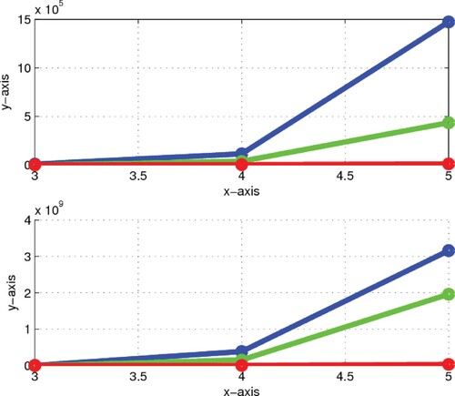
Figure 4. Comparison between bounds and exact values of FGZI $\mathrm{\&}$ GRI: In first graph ${\alpha }_1$ by green colour, exact value of FGZI by pink colour and ${\alpha }_2$ by purple colour are presented. Similarly, in second graph ${\text{β}}_1$ by purple colour, exact value of GRI by green colour and ${\text{β}}_2$ by red colour are presented.

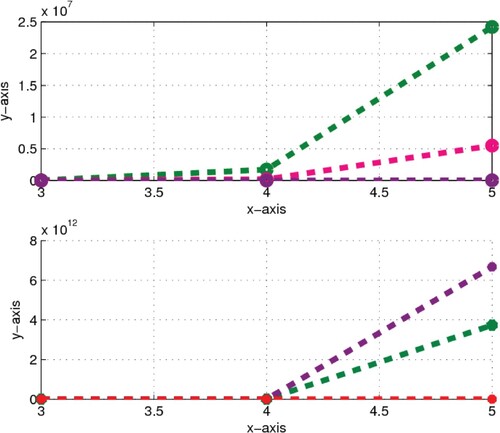
Figure 5. Comparison of bounds and exact values of FGZI $\mathrm{\&}$ GRI: In first graph ${\alpha }_1$ by blue colour, exact value of FGZI by purple colour and ${\alpha }_2$ by red colour are presented. In second graph, ${\text{β}}_1$ by purple colour, exact value of GRI by green colour and ${\text{β}}_2$ by red colour are presented.

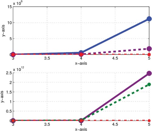
Figure 6. Comparison of bounds and exact values of FGZI $\mathrm{\&}$ GRI: In first graph ${\alpha }_1$ by green colour, exact value of FGZI by purple colour and ${\alpha }_2$ by red colour are presented. Similarly, in second graph, ${\text{β}}_1$ by purple colour, exact value of GRI by blue colour and ${\text{β}}_2$ by red colour are presented.

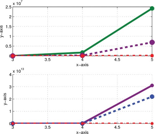
Table 1. $P_{n+S}{P}_m$.

$[\mathrm{m},\mathrm{n},\alpha ]$	${\alpha }_1$	${\alpha }_2$	${\text{β}}_1$	${\text{β}}_2$
(3,3,3)	7680	405	376,128	58752
(4,4,4)	114,688	2268	382,205,952	1,492,992
(5,5,5)	1,474,560	10,935	$3.159569203\times {10}^{10}$	30,855,168
(6,6,6)	1,730,1504	48,114	$2.323812188\times {10}^{12}$	567,336,960
(7,7,7)	190,840,832	199,017	$1.585084524\times {10}^{14}$	9,674,588,160

Table 2. $P_{n+R}{P}_m$.

$[\mathrm{m},\mathrm{n},\alpha ]$	${\alpha }_1$	${\alpha }_2$	${\text{β}}_1$	${\text{β}}_2$
(3,3,3)	41,160	960	100,018,800	1000
(4,4,4)	1,728,720	7168	$2.722111661\times {10}^{10}$	2160
(5,5,5)	24,202,080	46,080	$5.970498243\times {10}^{12}$	3760
(6,6,6)	496,949,376	270,336	$1.160436201\times {10}^{15}$	5800
(7,7,7)	9,592,628,864	1,490,944	$\phantom{1}2.08734462\times {10}^{17}$	8280

Table 3. $P_{n+Q}{P}_m$.

$[\mathrm{m},\mathrm{n},\alpha ]$	${\alpha }_1$	${\alpha }_2$	${\text{β}}_1$	${\text{β}}_2$
(3,3,3)	25,920	405	75,582,720	202,500
(4,4,4)	580,608	2268	$1.306069402\times {10}^{10}$	4860,000
(5,5,5)	11,197,440	10,935	$2.468491169\times {10}^{12}$	127,575,000

Table 4. $P_{n+T}{P}_m$.

$[\mathrm{m},\mathrm{n},\alpha ]$	${\alpha }_1$	${\alpha }_2$	${\text{β}}_1$	${\text{β}}_2$
(3,3,3)	41,160	1875	246,564,864	1,404,000
(4,4,4)	1,728,720	17,500	$1.051504312\times {10}^{11}$	106,920,000
(5,5,5)	24,202,080	140,625	$3.731385049\times {10}^{13}$	5,637,600,000

Table 5. Exact values for FGZI.

$[\mathrm{m},\mathrm{n},\alpha ]$	$P_{n+S}{P}_m$	$P_{n+R}{P}_m$	$P_{n+Q}{P}_m$	$P_{n+T}{P}_m$
(3,3,3)	1808	6414	3442	8048
(4,4,4)	37,260	208,104	102,800	258,412
(5,5,5)	434,888	5,505,322	1,845,182	6,915,616

Table 6. Exact values for GRI.

$[\mathrm{m},\mathrm{n},\alpha ]$	$P_{n+S}{P}_m$	$P_{n+R}{P}_m$	$P_{n+Q}{P}_m$	$P_{n+T}{P}_m$
(3,3,3)	749,996	15,117,156	3,449,783	22,339,261
(4,4,4)	153,484,294	$1.348702778\times {10}^{10}$	$1.547709854\times {10}^{10}$	$2.108187784\times {10}^{10}$
(5,5,5)	$1.959081971\times {10}^{10}$	$6.679134798\times {10}^{12}$	$3.091969925\times {10}^{12}$	$4.194036307\times {10}^{13}$

5. Conclusion

In this paper, we have computed the bounds (upper and lower) for FGZI and GRI of φ-sum graphs which are obtained by the strong product of $\phi \left(G\right)$ graph with another graph Γ, where $\phi \left(G\right)$ is constructed using four subdivision operations on the graph G. At the end, we also included the results for some particular families of graphs as the applications of the obtained results and concluded that the exact values satisfy the obtained bounds. More preciously, upper and lower bounds for FGZI and GRI of φ-sum graphs based on strong product are computed, where $\alpha ,\text{β}>0$. In addition, if we assume that $\alpha ,\text{β}<0$ then these bounds become ${\alpha }_1\le M^{\alpha }\left(G_{+\phi }\mathrm{\Gamma }\right)\le {\alpha }_2$ and ${\text{β}}_1\le R^{\text{β}}\left(G_{+\phi }\mathrm{\Gamma }\right)\le {\text{β}}_2$.

Acknowledgments

The author is deeply thankful to the editor and the reviewers for their valuable suggestions to improve the quality of this manuscript.

Disclosure statement

No potential conflict of interest was reported by the author(s).

Additional information

Funding

The research was supported by the National Natural Science Foundation of China [grant numbers 11971142, 11871202, 61673169, 11701176, 11626101, 11601485].

References

- Gutman I. Degree-based topological indices. Croat Chem Acta. 2013;86(4):351–361. doi: 10.5562/cca2294
- Javaid M, Cao J. Computing topological indices of probabilistic neural network. Neural Comput Appl. 2018;30(12):3869–3876. doi: 10.1007/s00521-017-2972-1
- Devillers J, Balaban AT. Topological indices and related descriptors in QSAR and QSPR. Amsterdam: Gordon and Breach Science Publishers; 1999.
- Randic M. Characterization of molecular branching. J Am Chem Soc. 1975;97(23):6609–6615. doi: 10.1021/ja00856a001
- Van Steen M. Graph theory and complex networks: an introduction. Maarten van Steen; 2010. 144p.
- Yan W, Yang BY, Yeh YN. The behavior of Wiener indices and polynomials of graphs under five graph decorations. Appl Math Lett. 2007;20(3):290–295. doi: 10.1016/j.aml.2006.04.010
- Eliasi M, Taeri B. Four new sums of graphs and their Wiener indices. Discrete Appl Math. 2009;157(4):794–803. doi: 10.1016/j.dam.2008.07.001
- Deng H, Sarala D, Ayyaswamy SK, et al. The Zagreb indices of four operations on graphs. Appl Math Comput. 2016;275:422–431.
- Liu JB, Javed S, Javaid M, et al. Computing first general Zagreb index of operations on graphs. IEEE Access. 2019;7:47494–47502. doi: 10.1109/ACCESS.2019.2909822
- Akhter S, Imran M. The sharp bounds on general sum-connectivity index of four operations on graphs. J Inequalities Appl. 2016;2016(1):102. doi: 10.1186/s13660-016-1048-6
- Ahmad M, Saeed M, Javaid M, et al. Exact formula and improved bounds for general sum-connectivity index of graph-operations. IEEE Access. 2019;7:167290–167299.
- Akhter S, Imran M. Computing the forgotten topological index of four operations on graphs. AKCE Int J Graphs Comb. 2017;14(1):70–79. doi: 10.1016/j.akcej.2016.11.012
- Lokesha V, Shetty BS, Ranjini PS, et al. New bounds for randic and GA indices. J Inequalities Appl. 2013;2013(1):180. doi: 10.1186/1029-242X-2013-180
- Das KC, Akgunes N, Togan M, et al. On the first Zagreb index and multiplicative Zagreb coindices of graphs. Anal Univ “Ovidius” Constanta-Seria Mat. 2016;24(1):153–176. doi: 10.1515/auom-2016-0008
- Lokesha V, Shruti R, Ranjini P, et al. On certain topological indices of nanostructures using Q (G) and R (G) operators. Commun Fac Sci Univ Ank Ser A1 Math Stat. 2018;67(2):178–187.
- Togan M, Yurttas A, Cevik AS, et al. Zagreb indices and multiplicative Zagreb indices of double graphs of subdivision graphs. TWMS J Appl Eng Math. 2019;9(2):404.
- Lokesha V, Shruti R, Cevik AS. M-polynomial of subdivision and complementary graphs of banana tree graph. J Int Math Virtual Inst. 2020;10(1):157–182.
- Cevik AS, Lokesha V, Jain S, et al. New results on the F-index of graphs based on corona-type products of graphs. Proc Jangjeon Math Soc. 2020;23(2):141–147.
- Das KC, Yurttas A, Togan M, et al. The multiplicative Zagreb indices of graph operations. J Inequalities Appl. 2013;2013(1):90. doi: 10.1186/1029-242X-2013-90
- Liu JB, Javaid M, Awais HM. Computing Zagreb indices of the subdivision-related generalized operations of graphs. IEEE Access. 2019;7:105479–105488.
- Awais H, Javaid M, Jamal M. Forgotten index of generalized F-sum graphs. J Prime Res Math. 2019;15:115–128.
- Sarala D, Deng H, Natarajan C, et al. F index of graphs based on four new operations related to the strong product. AKCE Int J Gr Comb. 2018. doi: 10.1016/j.akcej.2018.07.003
- West DB. Introduction to graph theory. Upper Saddle River (NJ): Prentice Hall; 1996.
- Zhang X, Awais HM, Javaid M, et al. Multiplicative Zagreb indices of molecular graphs. J Chem. 2019;5294198. doi: 10.1155/2019/5294198
- Awais HM, Javaid M, Raheem A. Hyper-Zagreb index of graphs based on generalized subdivision related operations. Punjab Univ J Math. 2020;52(5):89–103.
- Gutman I, Trinajstić N. Graph theory and molecular orbitals. Total π-electron energy of alternant hydrocarbons. Chem Phys Lett. 1972;17(4):535–538. doi: 10.1016/0009-2614(72)85099-1
- Randić M. Characterization of molecular branching. J Am Chem Soc. 1975;97(23):6609–6615. doi: 10.1021/ja00856a001
- Bollobàs B, Erdös P. Graphs of extremal weights. Ars Comb. 1998;50:225–233.
- Li X, Zheng J. A unified approach to the extremal trees for different indices. MATCH Commun Math Comput Chem. 2005;54(1):195–208.
- Ahmad H, Seadawy AR, Khan TA, et al. Analytic approximate solutions for some nonlinear parabolic dynamical wave equations. J Taibah Univ Sci. 2020;14(1):346–358. doi: 10.1080/16583655.2020.1741943
- Özkan YS, Yaar E, Seadawy AR. A third-order nonlinear Schrödinger equation: the exact solutions, group-invariant solutions and conservation laws. J Taibah Univ Sci. 2020;14(1):585–597. doi: 10.1080/16583655.2020.1760513
- Marin M, Othman MI, Seadawy AR, et al. A domain of influence in the Moore–Gibson–Thompson theory of dipolar bodies. J Taibah Univ Sci. 2020;14(1):653–660. doi: 10.1080/16583655.2020.1763664