Super electron acoustic propagations in critical plasma density

ABSTRACT

The propagation of some new electrostatic cnoidal, super-solitons, super-periodic and shocklike waves in Earth magneto-tail electron acoustic (EA) plasma at critical density has been investigated via MKP equation. These MKP solutions are obtained by the method of expansion Jacobian elliptic function (EMJEF). Numerous of the given solutions are significant on the observations of broadband electrostatic nonlinear noise forms in layers of magneto-tail.

KEYWORDS:

• MKP equation
• super-solutions
• Jacobian elliptic method
• magneto-tail plasma

2010 MATHEMATICS SUBJECT CLASSIFICATIONS:

• 35C08
• 35Q35
• 65Z05

1. Introduction

The existence of EA electrostatic excitations in laboratories has been perceived [1, 2]. Various surveillance in space plasma assured the electrostatic EA propagation in heliospheric shock, auroral-zone, magnetospheres, geomagnetic tail and broadband noises [3–10]. The EA generations were reported as an acoustic-kind having inertia specified by cold electron mass and restoring forces given by hot electrons pressure [11, 12]. Abdelwahed et al. studied the characteristic modulations of EAs in vortex-like electrons plasma by introducing time-fraction parameter which modified the soliton structures in nonlinear modified fraction equation [13]. Pakzad investigated the hot nonextensive electron effects on EA properties using geometric coordinates as spherical and cylindrical EAs [14]. It was advised that the spherical EA amplitudes become larger than the cylindrical EA amplitudes. In another study, the geometric EA characteristics were examined in critical nonlinear attitude by Gardner modified equations [15]. Several EA electrostatic applications in many space systems have been explored [16–20].

The effect of variable magnetic field on the dissipative EA propagation without using sources of dissipation has been studied. It was reported that the backward oscillatory shocks were formed in plasmas. Also, the properties of these waves were studied using numerical real data [21]. Fahad et al. studied the dispersion features of EA waves in non-relativistic quantum recoil with isotropic non-degenerate system. The coefficients of absorption for Landau damping were discussed for laser-produced plasmas [22]. Also, Yahia et al. investigated the head-on EA collisions in quasi-elastic case in magnetized nonthermal plasma. They studied some parameter effects on both the solitary EA solitons and collision phase in auroral zone of the Earth [23].

Recently, there is a huge development in analytical methods for getting solutions for NPDEs, see [24–36] and references therein. So, the aim of this work is to use one of these methods to introduce new solution forms applicable for auroral zone observations.

2. Physical model

By considering a fluid plasma includes cold electron fluid and two temperature thermal ions which is governed by normalized equations [17]: (1) $\begin{array}{rl}& \frac{\mathrm{\partial }{n}_{ec}}{\mathrm{\partial }t}+\frac{\mathrm{\partial }}{\mathrm{\partial }x}(n_{ec}{u}_{ecx})+\frac{\mathrm{\partial }}{\mathrm{\partial }y}(n_{ec}{u}_{ecy})=0,\end{array}$(1) (2) $\begin{array}{rl}& \frac{\mathrm{\partial }{u}_{ecx}}{\mathrm{\partial }t}+u_{ecx}\frac{\mathrm{\partial }}{\mathrm{\partial }x}(u_{ecx})+u_{ecy}\frac{\mathrm{\partial }}{\mathrm{\partial }y}(u_{ecx})-\frac{\mathrm{\partial }\varphi }{\mathrm{\partial }x}=0,\end{array}$(2) (3) $\begin{array}{rl}& \frac{\mathrm{\partial }{u}_{ecy}}{\mathrm{\partial }t}+u_{ecx}\frac{\mathrm{\partial }}{\mathrm{\partial }x}(u_{ecy})+u_{ecy}\frac{\mathrm{\partial }}{\mathrm{\partial }y}(u_{ecy})-\frac{\mathrm{\partial }\varphi }{\mathrm{\partial }y}=0,\end{array}$(3) (4) $\begin{array}{rl}& \frac{{\mathrm{\partial }}^2\varphi }{\mathrm{\partial }{x}^2}+\frac{{\mathrm{\partial }}^2\varphi }{\mathrm{\partial }{y}^2}-(n_{ec}-\mu \exp \left(\frac{-\varphi }{\mu +\nu \beta }\right)\\ & -\gamma \exp \left(\frac{-\beta \varphi }{\mu +\nu \beta }\right))=0,\end{array}$(4) where $T_h(T_l)$ is high (low) temperature ion at density μ, γ with $\beta =\frac{T_l}{T_h}$. Using stretched coordinates $\xi =ϵ(x-\lambda t),\tau ={ϵ}^{3}t,\eta ={ϵ}^{2}y,$ where ε is a small value and λ is the EA speed, the model reaches critical density $\mu ={\mu }_c$ which means that the nonlinear coefficient vanished. So, the modified-KP equation (mKP) reads: (5) $\frac{\mathrm{\partial }}{\mathrm{\partial }\xi }(\frac{\mathrm{\partial }\varphi }{\mathrm{\partial }\tau }+G{\varphi }^2\frac{\mathrm{\partial }\varphi }{\mathrm{\partial }\xi }+R\frac{{\mathrm{\partial }}^3\varphi }{\mathrm{\partial }{\xi }^3})+Q\frac{{\mathrm{\partial }}^2\varphi }{\mathrm{\partial }{\eta }^2}=0$(5) with (6) $\begin{array}{rl}{\mu }_c& =\frac{\begin{array}{c}-{\lambda }^4+{\beta }^2{\lambda }^4\pm (\beta -1){\lambda }^2\\ \sqrt{{\lambda }^4{\beta }^2+2\beta {\lambda }^4+{\lambda }^4-12\beta }-6\beta (\beta -1)\end{array}}{2(-3\beta (\beta -2)-3)},\end{array}$(6) (7) $\begin{array}{rl}G& =\frac{1}{2}\lambda (-\frac{3\nu {\beta }^2}{2(\mu +\nu \beta {)}^2}-\frac{3}{{\lambda }^4}-\frac{3\mu }{2(\mu +\nu \beta {)}^2}),\\ Q& =\frac{\lambda }{2},R=\frac{{\lambda }^3}{2}.\end{array}$(7) By using a similarity transformation in the form of (8) $\begin{array}{rl}\chi & =L\xi +M\eta -\tau ({\upsilon }_1+{\upsilon }_2),\end{array}$(8) (9) $\begin{array}{rl}\varphi (\chi )& =\varphi (x,y,t)\end{array}$(9) (10) $\begin{array}{rl}\tau & =t,\end{array}$(10) where L and M are directional cosines of x and y axes.

The transformed MKP equation to the ODE form is (11) $\begin{array}{rl}& \mathbf{3}\mathbf{(}\mathbf{S}\mathbf{-}\mathbf{v}\mathbf{)}\varphi \mathbf{+}\delta {\varphi }^3+\mathbf{3}\sigma \frac{{\mathrm{d}}^2\varphi }{\mathrm{d}{\chi }^2}=\mathbf{0},\end{array}$(11) (12) $\begin{array}{rl}& S=\frac{M^{2}Q}{L}-u,\delta =GL,\sigma =R{L}^3,\end{array}$(12) where u and v are travelling speeds in both directions.

3. Closed-form solutions

Now we give the closed form solutions for equation (13) ${\mathrm{\Lambda }}_1{\mathrm{\Xi }}^{\mathrm{\prime }\mathrm{\prime }}+{\mathrm{\Lambda }}_2{\mathrm{\Xi }}^3+{\mathrm{\Lambda }}_3\mathrm{\Xi }=0,$(13) based on the Jacobian elliptic functions [37, 38]. Balancing ${\mathrm{\Xi }}^{\mathrm{\prime }\mathrm{\prime }}$ and ${\mathrm{\Xi }}^3$, gives m = 1. Thus the solution of Equation (13(13) ${\mathrm{\Lambda }}_1{\mathrm{\Xi }}^{\mathrm{\prime }\mathrm{\prime }}+{\mathrm{\Lambda }}_2{\mathrm{\Xi }}^3+{\mathrm{\Lambda }}_3\mathrm{\Xi }=0,$(13) ) takes the form: (14) $\mathrm{\Xi }=a_0+a_{1}sn(\eta )+b_{1}cn(\eta ),$(14) where $a_0$, $a_1$ and $b_1$ are parameters. From Equation (14(14) $\mathrm{\Xi }=a_0+a_{1}sn(\eta )+b_{1}cn(\eta ),$(14) ), we get (15) $\begin{array}{rl}{\mathrm{\Xi }}^{\mathrm{\prime }}& =a_{1}cn(\eta )dn(\eta )-b_{1}sn(\eta )dn(\eta ),\end{array}$(15) (16) $\begin{array}{rl}{\mathrm{\Xi }}^{\mathrm{\prime }\mathrm{\prime }}& =-m^{2}sn(\eta )a_1+2a_{1}sn(\eta {)}^3{m}^2\\ & +2m^{2}sn(\eta {)}^{2}cn(\eta )b_1-a_{1}sn(\eta )-b_{1}cn(\eta ).\end{array}$(16) Superseding Equations (14(14) $\mathrm{\Xi }=a_0+a_{1}sn(\eta )+b_{1}cn(\eta ),$(14) )–(16(16) $\begin{array}{rl}{\mathrm{\Xi }}^{\mathrm{\prime }\mathrm{\prime }}& =-m^{2}sn(\eta )a_1+2a_{1}sn(\eta {)}^3{m}^2\\ & +2m^{2}sn(\eta {)}^{2}cn(\eta )b_1-a_{1}sn(\eta )-b_{1}cn(\eta ).\end{array}$(16) ) into Equation (13(13) ${\mathrm{\Lambda }}_1{\mathrm{\Xi }}^{\mathrm{\prime }\mathrm{\prime }}+{\mathrm{\Lambda }}_2{\mathrm{\Xi }}^3+{\mathrm{\Lambda }}_3\mathrm{\Xi }=0,$(13) ) and setting all coefficients of $s{n}^3$, $s{n}^2\mathit{c}\mathit{n}$, $s{n}^2$, $sn\mathit{c}\mathit{n}$, sn, cn, $s{n}^0$ to zero, gives a system of algebraic equations. Solving these equations, yields:

Case 1. $\begin{array}{rl}& a_0=0,a_1=\pm \sqrt{\frac{-2{\mathrm{\Lambda }}_1}{{\mathrm{\Lambda }}_2}}m,b_1=0,\\ & {\mathrm{\Lambda }}_3={\mathrm{\Lambda }}_1(1+m^2).\end{array}$ Hence the first family solution is (17) ${\mathrm{\Xi }}_1(x,t)=\pm \sqrt{\frac{-2{\mathrm{\Lambda }}_1}{{\mathrm{\Lambda }}_2}}msn(\eta ).$(17) When $m\to 1$, Equation (17(17) ${\mathrm{\Xi }}_1(x,t)=\pm \sqrt{\frac{-2{\mathrm{\Lambda }}_1}{{\mathrm{\Lambda }}_2}}msn(\eta ).$(17) ) becomes (18) ${\mathrm{\Xi }}_1(x,t)=\pm \sqrt{\frac{-2{\mathrm{\Lambda }}_1}{{\mathrm{\Lambda }}_2}}\tanh (\eta ).$(18) Case 2. $\begin{array}{rl}& a_0=0,a_1=\pm \sqrt{\frac{-{\mathrm{\Lambda }}_1}{2{\mathrm{\Lambda }}_2}}m,b_1=-\sqrt{\frac{{\mathrm{\Lambda }}_1}{2{\mathrm{\Lambda }}_2}}m,\\ & {\mathrm{\Lambda }}_3=\frac{1}{2}{\mathrm{\Lambda }}_1(2-m^2).\end{array}$ Hence the second family solution is (19) ${\mathrm{\Xi }}_2(x,t)=\pm \sqrt{\frac{-{\mathrm{\Lambda }}_1}{2{\mathrm{\Lambda }}_2}}msn(\eta )-\sqrt{\frac{{\mathrm{\Lambda }}_1}{2{\mathrm{\Lambda }}_2}}mcn(\eta ).$(19) When $m\to 1$, Equation (19(19) ${\mathrm{\Xi }}_2(x,t)=\pm \sqrt{\frac{-{\mathrm{\Lambda }}_1}{2{\mathrm{\Lambda }}_2}}msn(\eta )-\sqrt{\frac{{\mathrm{\Lambda }}_1}{2{\mathrm{\Lambda }}_2}}mcn(\eta ).$(19) ) becomes (20) ${\mathrm{\Xi }}_2(x,t)=\pm \sqrt{\frac{-{\mathrm{\Lambda }}_1}{2{\mathrm{\Lambda }}_2}}\tanh (\eta )-\sqrt{\frac{{\mathrm{\Lambda }}_1}{2{\mathrm{\Lambda }}_2}}\mathrm{sech}(\eta )$(20) Case 3. $\begin{array}{rl}& a_0=0,a_1=\pm \sqrt{\frac{-{\mathrm{\Lambda }}_1}{2{\mathrm{\Lambda }}_2}}m,b_1=\sqrt{\frac{{\mathrm{\Lambda }}_1}{2{\mathrm{\Lambda }}_2}}m,\\ & {\mathrm{\Lambda }}_3=\frac{1}{2}{\mathrm{\Lambda }}_1(2-m^2).\end{array}$ Hence the third family solution is (21) ${\mathrm{\Xi }}_3(x,t)=\pm \sqrt{\frac{-{\mathrm{\Lambda }}_1}{2{\mathrm{\Lambda }}_2}}msn(\eta )+\sqrt{\frac{{\mathrm{\Lambda }}_1}{2{\mathrm{\Lambda }}_2}}mcn(\eta ).$(21) When $m\to 1$, Equation (21(21) ${\mathrm{\Xi }}_3(x,t)=\pm \sqrt{\frac{-{\mathrm{\Lambda }}_1}{2{\mathrm{\Lambda }}_2}}msn(\eta )+\sqrt{\frac{{\mathrm{\Lambda }}_1}{2{\mathrm{\Lambda }}_2}}mcn(\eta ).$(21) ) becomes (22) ${\mathrm{\Xi }}_3(x,t)=\pm \sqrt{\frac{-{\mathrm{\Lambda }}_1}{2{\mathrm{\Lambda }}_2}}\tanh (\eta )+\sqrt{\frac{{\mathrm{\Lambda }}_1}{2{\mathrm{\Lambda }}_2}}\mathrm{sech}(\eta ).$(22) Case 4. $\begin{array}{rl}& a_0=0,a_1=0,b_1=\pm \sqrt{\frac{2{\mathrm{\Lambda }}_1}{{\mathrm{\Lambda }}_2}}m,\\ & {\mathrm{\Lambda }}_3={\mathrm{\Lambda }}_1(1-2m^2).\end{array}$ Hence the fourth family solution is (23) ${\mathrm{\Xi }}_4(x,t)=\pm \sqrt{\frac{2{\mathrm{\Lambda }}_1}{{\mathrm{\Lambda }}_2}}mcn(\eta ).$(23) As long as $m\to 1$, Equation (23(23) ${\mathrm{\Xi }}_4(x,t)=\pm \sqrt{\frac{2{\mathrm{\Lambda }}_1}{{\mathrm{\Lambda }}_2}}mcn(\eta ).$(23) ) becomes (24) ${\mathrm{\Xi }}_4(x,t)=\pm \sqrt{\frac{2{\mathrm{\Lambda }}_1}{{\mathrm{\Lambda }}_2}}sech(\eta ).$(24)

4. Results and discussion

In this section, we employed the closed-form solution to solve Equation (5). Comparing this equation with Equation (13(13) ${\mathrm{\Lambda }}_1{\mathrm{\Xi }}^{\mathrm{\prime }\mathrm{\prime }}+{\mathrm{\Lambda }}_2{\mathrm{\Xi }}^3+{\mathrm{\Lambda }}_3\mathrm{\Xi }=0,$(13) ) yields ${\mathrm{\Lambda }}_1=3\sigma$, ${\mathrm{\Lambda }}_2=\delta$ and ${\mathrm{\Lambda }}_3=-3(\upsilon -s)$. Thus the solutions of Equation (11(11) $\begin{array}{rl}& \mathbf{3}\mathbf{(}\mathbf{S}\mathbf{-}\mathbf{v}\mathbf{)}\varphi \mathbf{+}\delta {\varphi }^3+\mathbf{3}\sigma \frac{{\mathrm{d}}^2\varphi }{\mathrm{d}{\chi }^2}=\mathbf{0},\end{array}$(11) ) are:

Case 1. The first family of solution is (25) ${\varphi }_1(x,t)=\pm \sqrt{\frac{-6\sigma }{\delta }}msn(x-(s-\sigma (1+m^2))t),$(25) when $m\to 1$, the solutions of Equation (25(25) ${\varphi }_1(x,t)=\pm \sqrt{\frac{-6\sigma }{\delta }}msn(x-(s-\sigma (1+m^2))t),$(25) ) become (26) ${\varphi }_1(x,t)=\pm \sqrt{\frac{-6\sigma }{\delta }}\tanh (x-(s-2\sigma )t).$(26) Case 2. The second family of solution is (27) $\begin{array}{rl}{\varphi }_2(x,t)& =\pm \sqrt{\frac{-3\sigma }{2\delta }}msn(x-(s-\frac{1}{2}\sigma (2-m^2))t)\\ & -\sqrt{\frac{3\sigma }{2\delta }}mcn(x-(s-\frac{1}{2}\sigma (2-m^2))t).\end{array}$(27) When $m\to 1$, the solutions of Equation (27(27) $\begin{array}{rl}{\varphi }_2(x,t)& =\pm \sqrt{\frac{-3\sigma }{2\delta }}msn(x-(s-\frac{1}{2}\sigma (2-m^2))t)\\ & -\sqrt{\frac{3\sigma }{2\delta }}mcn(x-(s-\frac{1}{2}\sigma (2-m^2))t).\end{array}$(27) ) become (28) $\begin{array}{rl}{\varphi }_2(x,t)& =\pm \sqrt{\frac{-3\sigma }{2\delta }}\tanh (x-(s-\frac{1}{2}\sigma )t)\\ & -\sqrt{\frac{3\sigma }{2\delta }}\mathrm{sech}(x-(s-\frac{1}{2}\sigma )t).\end{array}$(28) Case 3. The third family of solutions is (29) $\begin{array}{rl}{\varphi }_3(x,t)& =\pm \sqrt{\frac{-3\sigma }{2\delta }}msn(x-(s-\frac{1}{2}\sigma (2-m^2))t)\\ & +\sqrt{\frac{3\sigma }{2\delta }}mcn(x-(s-\frac{1}{2}\sigma (2-m^2))t).\end{array}$(29) When $m\to 1$, the solutions of Equation (29(29) $\begin{array}{rl}{\varphi }_3(x,t)& =\pm \sqrt{\frac{-3\sigma }{2\delta }}msn(x-(s-\frac{1}{2}\sigma (2-m^2))t)\\ & +\sqrt{\frac{3\sigma }{2\delta }}mcn(x-(s-\frac{1}{2}\sigma (2-m^2))t).\end{array}$(29) ) become (30) $\begin{array}{rl}{\varphi }_3(x,t)& =\pm \sqrt{\frac{-3\sigma }{2\delta }}\tanh (x-(s-\frac{1}{2}\sigma )t)\\ & +\sqrt{\frac{3\sigma }{2\delta }}\mathrm{sech}(x-(s-\frac{1}{2}\sigma )t).\end{array}$(30) Case 4. The fourth family of solutions is (31) ${\varphi }_4(x,t)=\pm \sqrt{\frac{6\sigma }{\delta }}mcn(x-(s-\sigma (1-2m^2))t).$(31) When $m\to 1$, the solutions of Equation (31(31) ${\varphi }_4(x,t)=\pm \sqrt{\frac{6\sigma }{\delta }}mcn(x-(s-\sigma (1-2m^2))t).$(31) ) become (32) ${\varphi }_4(x,t)=\pm \sqrt{\frac{6\sigma }{\delta }}\mathrm{sech}(x-(s+\sigma )t).$(32) In thermal plasma mode, two dimension EA solitons are described by the MKP equation (5(5) $\frac{\mathrm{\partial }}{\mathrm{\partial }\xi }(\frac{\mathrm{\partial }\varphi }{\mathrm{\partial }\tau }+G{\varphi }^2\frac{\mathrm{\partial }\varphi }{\mathrm{\partial }\xi }+R\frac{{\mathrm{\partial }}^3\varphi }{\mathrm{\partial }{\xi }^3})+Q\frac{{\mathrm{\partial }}^2\varphi }{\mathrm{\partial }{\eta }^2}=0$(5) ). The EA solutions have been examined using parameters for Earth magneto-tails [16, 17]. At $\mu ={\mu }_c$, MKP solutions can depict the system features using EMJEF method which allows many solution groups. 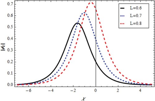Equation (25(25) ${\varphi }_1(x,t)=\pm \sqrt{\frac{-6\sigma }{\delta }}msn(x-(s-\sigma (1+m^2))t),$(25) ) is a solution group ${\varphi }_c=q_1(x;t)$ which have solutions depend on the model constants and parameters as shown in Figures 1–4. The first solution is cnoidal wave potential plotted for varying χ and L.as shown in Figures 1 and 2. It was founded that the cnoidal amplitude increases by L with positive phase change for $\lambda =1$ and negative phase change for $\lambda =-1$. The second solution introduces a shock wave as in Figures 3 and 4. It was shown that the shock amplitude increases by L with negative phase change for $\lambda =1$ and positive phase change for $\lambda =-1$. Equations (27(27) $\begin{array}{rl}{\varphi }_2(x,t)& =\pm \sqrt{\frac{-3\sigma }{2\delta }}msn(x-(s-\frac{1}{2}\sigma (2-m^2))t)\\ & -\sqrt{\frac{3\sigma }{2\delta }}mcn(x-(s-\frac{1}{2}\sigma (2-m^2))t).\end{array}$(27) ) and (29(29) $\begin{array}{rl}{\varphi }_3(x,t)& =\pm \sqrt{\frac{-3\sigma }{2\delta }}msn(x-(s-\frac{1}{2}\sigma (2-m^2))t)\\ & +\sqrt{\frac{3\sigma }{2\delta }}mcn(x-(s-\frac{1}{2}\sigma (2-m^2))t).\end{array}$(29) ) are various solutions ${\varphi }_c=q_2(x;t)$ and ${\varphi }_c=q_3(x;t)$ that distinguish diverse solitary waveforms. On the other hand, an important solitary forms ${\varphi }_c=q_4(x;t)$ Equation (31(31) ${\varphi }_4(x,t)=\pm \sqrt{\frac{6\sigma }{\delta }}mcn(x-(s-\sigma (1-2m^2))t).$(31) ) which have three solutions. The potential change with χ and L is shown in Figures 5–10. Figures 5 and 6 represent the soliton train. Moreover, super-solitary and soliton structures are given in Figures 7–10. Consequently, for all structures of Equation (31(31) ${\varphi }_4(x,t)=\pm \sqrt{\frac{6\sigma }{\delta }}mcn(x-(s-\sigma (1-2m^2))t).$(31) ), it was assured that the direction parameter L increases the train, super-solitary and soliton amplitudes with negative changes in wave phase for $\lambda =1$ and positive changes in wave phase for $\lambda =-1$ as depicted in Figures 7–10.

Figure 1. Change of periodic ${\varphi }_c=q_1(x;t)$ with $\chi ,L$ for $\beta =0.05,u=0.5,v=0.5,\lambda =1$.

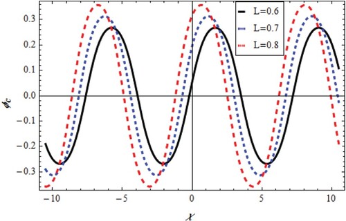
Figure 2. Change of periodic ${\varphi }_c=q_1(x;t)$ with $\chi ,L$ for $v=0.5,u=0.5,\beta =0.05,\lambda =-1$.

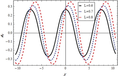
Figure 3. Change of shock ${\varphi }_c=q_1(x;t)$ with $\chi ,L$ for $v=0.5,u=0.5,\beta =0.05,\lambda =1$.

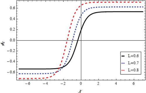
Figure 4. Change of shock ${\varphi }_c=q_1(x;t)$ with $\chi ,L$ for $v=0.5,u=0.5,\beta =0.05,\lambda =-1$.

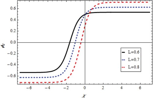
Figure 5. Change of solitary train ${\varphi }_c=q_4(x;t)$ with $\chi ,L$ for $v=0.5,u=0.5,\beta =0.05,\lambda =1$.

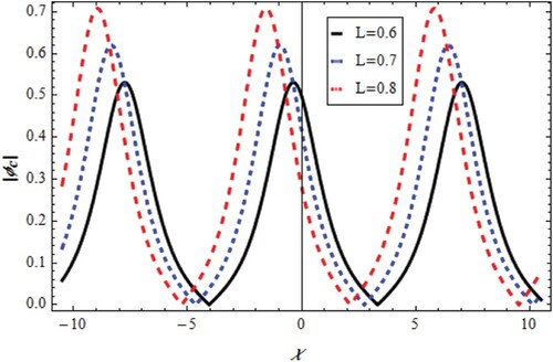
Figure 6. Change of solitary train ${\varphi }_c=q_4(x;t)$ with $\chi ,L$ for $v=0.5,u=0.5,\beta =0.05,\lambda =-1$.

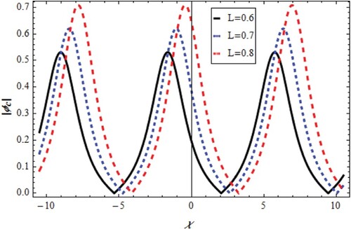
Figure 7. Change of super soliton ${\varphi }_c=q_4(x;t)$ with $\chi ,L$ for $v=0.5,u=0.5,\beta =0.05,\lambda =1$.

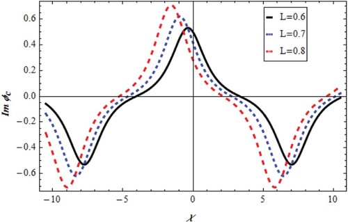
Figure 8. Change of super soliton ${\varphi }_c=q_4(x;t)$ with $\chi ,L$ for $v=0.5,u=0.5,\beta =0.05,\lambda =-1$.

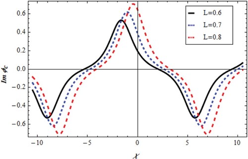
Figure 9. Change of soliton ${\varphi }_c=q_4(x;t)$ with $\chi ,L$ for $v=0.5,u=0.5,\beta =0.05,\lambda =1$.

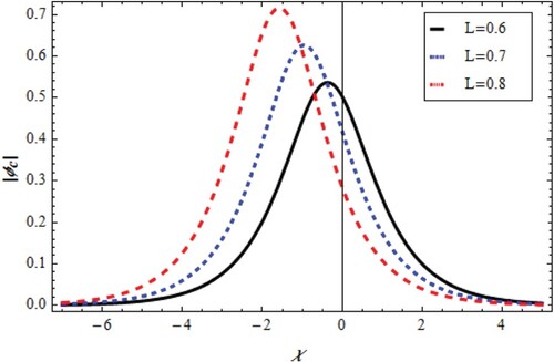
Figure 10. Change of soliton ${\varphi }_c=q_4(x;t)$ with $\chi ,L$ for $v=0.5,u=0.5,\beta =0.05,\lambda =-1$.

5. Conclusion

Using EMJEF technique, several wave generations such as solitons, cnoidal, shocks, solitary trains and super-solitons are characterized by the MKP equation that defined EA progress in thermal plasma mode. It was confirmed that the L direction can raise wave amplitude in plasma system, Otherwise, EA speed λ is controlled by the wave phase. So, the obtained results may apply to study the EA electrostatic observations and broadband magneto-tails.

Acknowledgements

This project was supported by the deanship of scientific research at Prince Sattam Bin Abdulaziz University under the research project No. 17450 /01/2020.

Disclosure statement

No potential conflict of interest was reported by the author(s).

References

- Henry D, Treguier JP. Propagation of electronic longitudinal modes in a non-Maxwellian plasma. J Plasma Phys. 1972;8:311–319.
- Ikezawa S, Nakamura Y. Observation of electron plasma waves in plasma of two-temperature electrons. J Phys Soc Jpn. 1981;50:962–967.
- Dubouloz N, Pottelette R, Malingre M, et al. Generation of broadband electrostatic noise by electron acoustic solitons. Geophys Res Lett. 1991;18:155–158.
- Singh SV, Lakhina GS. Generation of electron-acoustic waves in the magnetosphere. Planet Space Sci. 2001;49:107–114.
- Dubouloz N, Treumann RA, Pottelette R, et al. Turbulence generated by a gas of electron acoustic solitons. Geophys Res. 1993;98:17415–17422.
- Gill TS, Kaur H, Bansal S, et al. Modulational instability of electron-acoustic waves: an application to auroral zone plasma. Eur Phys J D. 2007;41(1):151–156.
- Demiray H. Modulation of electron-acoustic waves in a plasma with kappa distribution. Phys Plasmas. 2016;23:032109.
- Devanandhan S, Singh SV, Lakhina GS, et al. Electron acoustic waves in a magnetized plasma with kappa distributed ions. Phys Plasmas. 2012;19:082314.
- Williams G, Verheest F, Hellberg MA, et al. A Schamel equation for ion acoustic waves in superthermal plasmas. Phys Plasmas. 2014;21:092103.
- Abdelwahed HG. Higher-order corrections to broadband electrostatic shock noise in auroral zone. Phys Plasmas. 2015;22:092102.
- Fried BD, Gould RW. Longitudinal ion oscillations in a hot plasma. Phys Fluids. 1961;4:139.
- Watanabe K, Taniuti T. Electron-acoustic mode in a plasma of two-temperature electrons. J Phys Soc Jpn. 1977;43:1819–1820.
- Abdelwahed HG, El-Shewy EK, Mahmoud AA. Cylindrical electron acoustic solitons for modified time-fractional nonlinear equation. Phys Plasmas. 2017;24:082107.
- Pakzad HR. Cylindrical and spherical electron acoustic solitary waves with nonextensive hot electrons. Phys Plasmas. 2011;18:082105.
- Shuchy ST, Mannan A, Mamun AA. Cylindrical and spherical electron-acoustic Gardner solitons and double layers in a two-electron-temperature plasma with nonthermal ions. JETP Lett. 2012;95(6):282–288.
- Matsumoto H, Kojima H, Miyatake T, et al. Electrostatic solitary waves (ESW) in the magnetotail: BEN wave forms observed by GEOTAIL. Geophys Res Lett. 1994;21:2915–2918.
- Elwakil SA, El-hanbaly AM, El-Shewy EK, et al. Electron acoustic soliton energy of the Kadomtsev–Petviashvili equation in the Earth's magnetotail region at critical ion density. Astrophys Space Sci. 2014;349:197–203.
- Aliyu AI, Li Y, Qi L, et al. Lump-type and bell-shaped soliton solutions of the time-dependent coefficient Kadomtsev–Petviashvili equation. Front Phys. 2020;7:242. doi:10.3389/fphy.2019.00242
- Abdo NF. Effect of non Maxwellian distribution on the dressed electrostatic wave and energy properties. J Taibah Univ Sci. 2017;11:617–622.
- El-Shewy EK, Abdelwahed HG, Abdo NF, et al. On the modulation of ionic velocity in electron-positron-ion plasmas. J Taibah Univ Sci.2017;11:1267–1274.
- Pakzad HR, Javidan K, Eslami P. Electron acoustic waves in atmospheric magnetized plasma. Phys Scr.2020;95:045605.
- Fahad S, Ahmad M, Jan Q, et al. Dispersion properties of electron acoustic waves in degenerate and non-degenerate quantum plasmas. Contrib Plasma Phys.2019;59(10):41.
- Yahia ME, El-Labanym SK, Sabry R, et al. Head-On collision of electron-acoustic solitons in a magnetized plasma. IEEE Trans Plasma Sci2019;47(1):762–769.
- Abdelrahman MAE, Sohaly MA. On the new wave solutions to the MCH equation. Indian J Phys.2019;93:903–911.
- Abdelrahman MAE, Sohaly MA. The development of the deterministic nonlinear PDEs in particle physics to stochastic case. Results Phys. 2018;9:344–350.
- Abdelrahman MAE. A note on Riccati–Bernoulli sub-ODE method combined with complex transform method applied to fractional differential equations. Nonlinear Eng. 2018;7(4):279–285.
- Hassan SZ, Abdelrahman MAE. A Riccati Bernoulli sub-ODE method for some nonlinear evolution equations. Int J Nonlinear Sci Numer Simul.2019;20(3–4):303–313.
- Hassan SZ, Abdelrahman MAE. Solitary wave solutions for some nonlinear time fractional partial differential equations. Pramana J Phys. 2018;91:67.
- Abdelrahman MAE, Sohaly MA. Solitary waves for the nonlinear Schrödinger problem with the probability distribution function in stochastic input case. Eur Phys J Plus. 2017;132:339.
- Hassan SZ, Alyamani NA, Abdelrahman MAE. A construction of new traveling wave solutions for the 2D Ginzburg–Landau equation. Eur Phys J Plus 2019;134:425.
- Abdelrahman MAE, Abdo NF. On the nonlinear new wave solutions in unstable dispersive environments. Phys Scr. 2020;95(4):045220.
- Abdelrahman MAE, AlKhidhr HA. A robust and accurate solver for some nonlinear partial differential equations and tow applications. Phys Scr. 2020;95:065212.
- Baskonus HM, Bulut H. New wave behaviors of the system of equations for the ion sound and Langmuir waves. Waves Random Complex Media. 2016;26:613–625.
- Liu C. Exact solutions for the higher-order nonlinear Schrödinger equation in nonlinear optical fibres. Chaos Solitons Fractals. 2005;23:949–955.
- Zhang S. Exp-function method for solving Maccari's system. Phys Lett A. 2007;371:65–71.
- Bulut H, Sulaiman TA, Baskonus HM. Optical solitons to the resonant nonlinear Schrödinger equation with both spatio-temporal and inter-modal dispersions under Kerr law nonlinearity. Optik2018;163:49–55.
- Dai CQ, Zhang JF. Jacobian elliptic function method for nonlinear differential-difference equations. Chaos Solutions Fractals2006;27:1042–1047.
- Wanga Q, Chen Y, Zhang H. An extended Jacobi elliptic function rational expansion method and its application to (2+1)-dimensional dispersive long wave equation. Phys Lett A. 2005;340:411–426.