Dynamical behaviours and soliton solutions of the conformable fractional Schrödinger–Hirota equation using two different methods

Abstract

The nonlinear conformable fractional Schrödinger–Hirota (NCFSH) equation, describing the propagation of optical solitons in a dispersive optical fibre, is considered and its exact solutions are investigated. Abundant solutions including dark, bright and singular solutions have been obtained by two distinct methods, namely direct method and trial equation method. These methods provide a direct and efficient strategy for the NCFSH equation. The solutions have been simulated by graphs to check the types of solitons and their dynamical behaviours. With back substitution using Mathematica, all the solutions have been verified. Obtaining optical solutions to the proposed equation will play a fundamental role due to the applications in quantum mechanics, fluid dynamics, nonlinear optics and various other branches of mathematical physics.

KEYWORDS:

• Fractional Schrödinger–Hirota equation
• conformable derivative
• optical solutions

1. Introduction

In recent times, fractional derivatives are more preferred than classical derivatives to model real-world problems. Fractional derivatives are commonly seen in conservative and nonconservative phenomena. To model processes consisting of electromagnetic waves, electro-electrolyte polarization, diffusion wave and heat conduction, etc. fractional derivatives can be used [1].

The class of Schrödinger equations is generally modelled phenomenon, especially in quantum mechanics, energy and energy quantization. The linear Schrödinger equation represents the time evolution of wave function, whereas the nonlinear form is the most common equation for the evolution of slowly changing quasi-monochrome wave packets in weak nonlinear media with dispersion [2]. It models various nonlinearity effects in fibre such as self-phase modulation, second harmonic generation, ultrashort pulses, optical solitons, four-wave mixing, stimulated Raman scattering and so on. Laskin proposed the fractional Schrödinger equation which is an essential equation of fractional quantum mechanics [3].

In this paper, the nonlinear conformable fractional Schrödinger–Hirota (NCFSH) equation is considered as [4–7] (1) $\begin{array}{r}i{u}_t^{(\mu )}+\frac{1}{2}{u}_{xx}+|u{|}^{2}u+i\lambda u_{xxx}=0,t\ge 0,0<\mu \le 1.\end{array}$(1) The NCFSH equation describes real-world models in nonlinear optics and dispersive optical fibres [6,7]. Due to the applications in various fields, especially in optical communication systems, this equation and its solutions which enable to interperet the phenomena it represents taken much attention recently.

For the fractional operator, many approaches are known based on Gamma function. Therefore, in Equation (1), the fractional operator is considered the conformable derivative operator [8]. Most of the properties of the conformable derivative correspond to the classical derivative [9] and this definition allows to solve nonlinear partial fractional differential equations (NPFDEs) more easily [10].

The conformable derivative of order $\mu$ for the function $f$ is given by [8] (2) $T_{\mu }(f)(t)=\underset{\epsilon \to 0}{lim}\frac{f(t+\epsilon t^{1-\mu })-f(t)}{\epsilon },$(2) where $f:[0,\mathrm{\infty })\to R$, $\mathrm{\forall }t>0,\mu \in (0,1)$.

All of the classical derivative rules, such as linearity, sum, product, division, etc. are same as the conformable derivative. Additionally, if $\mu \in (0,1)$ and $f$ is differentiable, $T_{\mu }(f)(t)=t^{1-\mu }\frac{df}{dt}$can be determined [8]. Some authors [11,12] studied conformable fractional derivative and integral operators and gave geometric meaning of the conformable derivative [13]. The analysis of asymptotical stability for conformable fractional systems is given in recently published paper [14]. Recent studies [15–17] show attention to the conformable fractional derivative and its applications.

In order to find the numerical and analytical solutions of NPDEs, variety of approaches are proposed such as $G^{\mathrm{\prime }}/G$-expansion method [18,19], tanh-method [20,21], auxiliary equation method [22], simplest equation method [23], sub-equation method [24], hyperbolic function method [25], exponential rational function technique [26], ILC method [27], Picard operators method [28], invariant subspace method [29], Adomian decomposition method [30], exp-function method [31] and so on. More recently, Bernoulli approximation method and trial solution method are efficiently used in [32–36] to find exact solutions of fractional equations in physics and biology.

In this work, in addition to studies in [4–7], the TEM and the direct method are considered in the view of the definition and rules of the conformable derivative to attain the analytical solutions of the NCFSH equation.

2. Briefs of methods and results

In this section, briefs of methods and results obtained with these methods are given.

2.1. Trial equation method (TEM)

First, a nonlinear PDE, (3) $P(u,u_t,u_x,u_{xx},u_{tt},u_{xt},\dots )=0,$(3) is reduced to an ordinary differential equation, (4) $N(\xi ,z,z^{\mathrm{\prime }},z^{\mathrm{\prime }\mathrm{\prime }},\dots )=0,$(4) under the transformation $u(x,t)=z(\xi ),\xi =x-c(t^{\mu }/\mu ).$Second, consider the trial equation (5) $(z^{\mathrm{\prime }}{)}^2=\sum _{i=0}^n{a}_i{z}^i,$(5) where $a_i$ and $n$ are constants, which are derived from the solution of the system and the balancing principle, respectively.

Finally, the solution of Equation (5) can be given by the integral form (6) $\pm (\xi -{\xi }_0)=\int \frac{1}{\sqrt{\sum _{i=0}^n{a}_i{z}^i}}\text{d}z.$(6) The roots of the denominator can be classified and Equation (6) can be solved by a complete discrimination system for polynomial. Therefore, the exact solution of Equation (3) is hold [32].

Also, the trial equation can be chosen as (7) $z^{\mathrm{\prime }}=F(z)=\frac{G(z)}{H(z)}=\frac{a_r{z}^r+\dots +a_{1}z+a_0}{b_s{z}^s+\dots +b_{1}z+b_0}$(7) in the modified trial equation method [33,34], then the same procedure can be applied with the integral form solution of Equation (7) as (8) $\pm (\xi -{\xi }_0)=\int \frac{H(z)}{G(z)}\text{d}z.$(8) Similarly, one can solve integral (8) and find the exact travelling wave solutions of Equation (3).

2.1.1. Results for NCFSH Equation via the TEM

Consider the suitable wave transformation (9) $u(x,t)=z(\xi )e^{i\left(kx+\eta \frac{t^{\mu }}{\mu }\right)},\xi =x-2k\frac{t^{\mu }}{\mu },$(9) where $k$ and $\eta$ are constants. Using the above transformations and substituting the derivatives in Equation (1), and in point of the real and imaginary parts [7], $k=-1/3\lambda$ is obtained. Also, $z(\xi )$ satisfies the following ordinary differential equation: (10) $-\left(\frac{5}{54{\lambda }^2}+\eta \right)z+\frac{3}{2}{z}^{\mathrm{\prime }\mathrm{\prime }}+z^3=0.$(10)

Balancing $z^{\mathrm{\prime }\mathrm{\prime }}$ and $z^3$, we obtain $n=4$. So, trial equation is (11) $(z^{\mathrm{\prime }}{)}^2=a_0+a_{1}z+a_2{z}^2+a_3{z}^3+a_4{z}^4.$(11) Using the solution procedure of the algorithm yields a system of algebraic equations: $\begin{array}{l}81{\lambda }^2{a}_1=0,\\ -10-108\eta {\lambda }^2+162{\lambda }^2{a}_2=0,\\ 243{\lambda }^2{a}_3=0,\\ 108{\lambda }^2+324{\lambda }^2{a}_4=0.\end{array}$As a result of the system, coefficients are determined as (12) $\begin{array}{r}{a}_0=a_0,a_1=0,a_2=\frac{2\eta }{3}+\frac{5}{81{\lambda }^2},a_3=0,a_4=-\frac{1}{3}.\end{array}$(12) Equation (6) is rewritten with Equation (12), (13) $\begin{array}{r}\pm (\xi -{\xi }_0)=\int \frac{1}{\sqrt{a_0+\left(\frac{2\eta }{3}+\frac{5}{81{\lambda }^2}\right)z^2-\frac{1}{3}{z}^4}}\text{d}z.\end{array}$(13) If we set $a_0=0$ in Equation (13) and integrate this equation, the exact solutions of Equation (1) are obtained:

If $\frac{2\eta }{3}+\frac{5}{81{\lambda }^2}>0$, then we have bright and singular solutions, respectively: (14) $\begin{array}{rl}u(x,t)& =\pm \sqrt{2\eta +\frac{5}{27{\lambda }^2}}\\ & \times sech\left[\sqrt{\frac{2\eta }{3}+\frac{5}{81{\lambda }^2}}\left(x+\frac{2}{3\lambda }\frac{t^{\mu }}{\mu }\right)\right]e^{i\left(\frac{-1}{3\lambda }x+\eta \frac{t^{\mu }}{\mu }\right)},\end{array}$(14) (15) $\begin{array}{rl}u(x,t)& =\pm \sqrt{-\left(2\eta +\frac{5}{27{\lambda }^2}\right)}\\ & \times csch\left[\sqrt{\frac{2\eta }{3}+\frac{5}{81{\lambda }^2}}\left(x+\frac{2}{3\lambda }\frac{t^{\mu }}{\mu }\right)\right]e^{i\left(\frac{-1}{3\lambda }x+\eta \frac{t^{\mu }}{\mu }\right)}.\end{array}$(15) If $\frac{2\eta }{3}+\frac{5}{81{\lambda }^2}<0$, the singular periodic solutions appear as (16) $\begin{array}{rl}u(x,t)& =\pm \sqrt{2\eta +\frac{5}{27{\lambda }^2}}\\ & \times \sec \left[\sqrt{-\left(\frac{2\eta }{3}+\frac{5}{81{\lambda }^2}\right)}\left(x+\frac{2}{3\lambda }\frac{t^{\mu }}{\mu }\right)\right]\\ & \times e^{i\left(\frac{-1}{3\lambda }x+\eta \frac{t^{\mu }}{\mu }\right)},\end{array}$(16) (17) $\begin{array}{rl}u(x,t)& =\pm \sqrt{2\eta +\frac{5}{27{\lambda }^2}}\\ & \times \csc \left[\sqrt{-\left(\frac{2\eta }{3}+\frac{5}{81{\lambda }^2}\right)}\left(x+\frac{2}{3\lambda }\frac{t^{\mu }}{\mu }\right)\right]\\ & \times e^{i\left(\frac{-1}{3\lambda }x+\eta \frac{t^{\mu }}{\mu }\right)}.\end{array}$(17) Figures 1–3 show the nature of proposed solutions.

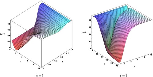
Figure 1. Behaviour of $|u(x,t){|}^2$ for solution (14) at $\lambda =-1,\eta =1$ and $\mu =0.4,0.8$, respectively.

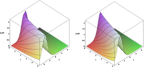
Figure 2. The solution (14) for different values of $\mu$ at $t=0.6$.

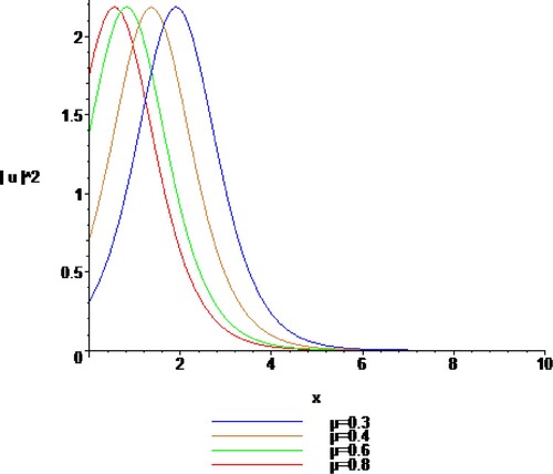
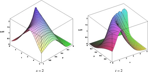
Figure 3. The solution (14) for fixed values of $x$ and $t$, respectively.

We now consider the modified form of the method to solve Equation (1).

If we now use the trial Equation (7) in Equation (10) for balancing procedure, we get $r-s=2$. Choosing $r=2$ and $s=0$, the trial equation is (18) $z^{\mathrm{\prime }}=\frac{a_0+a_{1}z+a_2{z}^2}{b_0}$(18) The corresponding system is: $\begin{array}{l}81{\lambda }^2{a}_0{a}_1=0,\\ 81{\lambda }^2{a}_1^2+162{\lambda }^2{a}_0{a}_2-5b_0^2-54\eta {\lambda }^2{b}_0^2=0,\\ 243{\lambda }^2{a}_1{a}_2=0,\\ 162{\lambda }^2{a}_2^2+54{\lambda }^2{b}_0^2=0.\end{array}$Solving the corresponding system, we obtain (19) $\begin{array}{r}{a}_0=\pm \frac{i{b}_0(5+54\eta {\lambda }^2)}{54\sqrt{3}{\lambda }^2},a_1=0,a_2=\mp \frac{i{b}_0}{\sqrt{3}},b_0=b_0.\end{array}$(19) Using these coefficients in Equation (8), we get (20) $\pm (\xi -{\xi }_0)=\int \frac{b_0}{\pm \frac{i{b}_0(5+54\eta {\lambda }^2)}{54\sqrt{3}{\lambda }^2}\mp \frac{i{b}_0}{\sqrt{3}}{z}^2}\text{d}z.$(20) When we integrate this equation and use the wave transformation, the exact travelling wave solutions of Equation (1) are obtained as follows:

If $\frac{5}{2}+27\eta {\lambda }^2<0$, then we have dark optical solutions: (21) $\begin{array}{rl}u(x,t)& =\pm \frac{i}{3\lambda }\sqrt{-\frac{5}{6}-9\eta {\lambda }^2}\\ & \times \tanh \left[\frac{1}{9\lambda }\sqrt{-\frac{5}{2}-27\eta {\lambda }^2}\left(x+\frac{2}{3\lambda }\frac{t^{\mu }}{\mu }+{\xi }_0\right)\right]\\ & \times e^{i\left(\frac{-1}{3\lambda }x+\eta \frac{t^{\mu }}{\mu }\right)},\end{array}$(21) (22) $\begin{array}{rl}u(x,t)& =\pm \frac{i}{3\lambda }\sqrt{-\frac{5}{6}-9\eta {\lambda }^2}\\ & \times \coth \left[\frac{1}{9\lambda }\sqrt{-\frac{5}{2}-27\eta {\lambda }^2}\left(x+\frac{2}{3\lambda }\frac{t^{\mu }}{\mu }+{\xi }_0\right)\right]\\ & \times e^{i\left(\frac{-1}{3\lambda }x+\eta \frac{t^{\mu }}{\mu }\right)}.\end{array}$(22) If $\frac{5}{2}+27\eta {\lambda }^2>0$, then the solutions purport periodic solutions: (23) $\begin{array}{rl}u(x,t)& =\pm \frac{i}{3\lambda }\sqrt{\frac{5}{6}+9\eta {\lambda }^2}\\ & \times \tan \left[\frac{1}{9\lambda }\sqrt{\frac{5}{2}+27\eta {\lambda }^2}\left(x+\frac{2}{3\lambda }\frac{t^{\mu }}{\mu }+{\xi }_0\right)\right]\\ & \times e^{i\left(\frac{-1}{3\lambda }x+\eta \frac{t^{\mu }}{\mu }\right)},\end{array}$(23) (24) $\begin{array}{rl}u(x,t)& =\pm \frac{i}{3\lambda }\sqrt{\frac{5}{6}+9\eta {\lambda }^2}\\ & \times \cot \left[\frac{1}{9\lambda }\sqrt{\frac{5}{2}+27\eta {\lambda }^2}\left(x+\frac{2}{3\lambda }\frac{t^{\mu }}{\mu }+{\xi }_0\right)\right]\\ & \times e^{i\left(\frac{-1}{3\lambda }x+\eta \frac{t^{\mu }}{\mu }\right)}.\end{array}$(24) Figures 4–6 show the graph of the corresponding solutions for the proposed equation.

Figure 4. Behaviour of $|u(x,t){|}^2$ for solution (21) at $\lambda =-1,\eta =1$, and $\mu =0.4,0.8$ respectively.

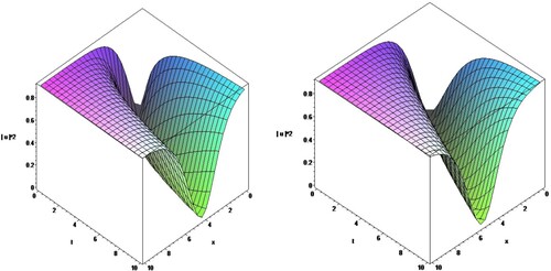
Figure 5. The solution (21) for different values of $\mu$ at $t=0.6$.

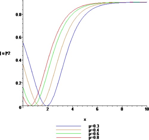
Figure 6. The solution (21) for fixed values of $x$ and $t$, respectively.

2.2. Direct method

If $f$ is differentiable, to reduce NPFDEs, the following rule of conformable fractional derivative, $T_{\alpha }(f)(t)=t^{1-\alpha }\frac{df}{dt},$can be used with the transformation $u(x,t)=z(\xi )e^{i(\sigma (\xi )-ct)},\xi =x-mt.$As a result, the reduced equation is nonlinear ordinary differential equation.

The reduced equation can be solved via analytical, semi-analytical and numerical methods.

2.2.1. Results for NCFSH equation via the direct method

Now, we consider the direct method to obtain analytical solutions of the NCFSH equation.

With conformable fractional derivative property, from Equation(1), (25) $\begin{array}{r}i{t}^{1-\mu }{u}_t+\frac{1}{2}{u}_{xx}+|u{|}^{2}u+i\lambda u_{xxx}=0,t\ge 0,0<\mu \le 1,\end{array}$(25) is obtained.

Case 1: With the transformation $u(x,t)=z(\xi )e^{i(x-ct)},\xi =x-mt,$the following equations are attained due to imaginary and real parts, respectively: (26) $\begin{array}{rl}\lambda z^{\mathrm{\prime }\mathrm{\prime }\mathrm{\prime }}-(m{t}^{1-\mu }+3\lambda -1)z^{\mathrm{\prime }}& =0,\end{array}$(26) (27) $\begin{array}{rl}\left(\frac{1}{2}-3\lambda \right)z^{\mathrm{\prime }\mathrm{\prime }}-\frac{1}{2}{z}^{\mathrm{\prime }}+(c{t}^{1-\mu }+\lambda )z+z^3& =0.\end{array}$(27) The analytical solution of the first equation is (28) $\begin{array}{rl}z(\xi )& =C_1+C_2\exp \left(\frac{\xi \sqrt{m{t}^{1-\mu }+3\lambda -1}}{\sqrt{\lambda }}\right)\\ & +C_3\exp \left(-\frac{\xi \sqrt{m{t}^{1-\mu }+3\lambda -1}}{\sqrt{\lambda }}\right).\end{array}$(28) Substituting the analytical solution $z(\xi )$ into the second equation and setting the coefficients of exponential function to zero gives the following system: $\begin{array}{rl}& 3{C_1}^2{C}_2\sqrt{\lambda }+C_2{\lambda }^{3/2}+3{C_2}^2{C}_3\sqrt{\lambda }+c{C}_2{t}^{1-\mu }\sqrt{\lambda }\\ & -3C_2\lambda \sqrt{m{t}^{1-\mu }+3\lambda -1}=0,\\ & 3{C_3}^2{C}_2\sqrt{\lambda }+C_3{\lambda }^{3/2}+3{C_1}^2{C}_3\sqrt{\lambda }+c{C}_3{t}^{1-\mu }\sqrt{\lambda }\\ & -3C_3\lambda \sqrt{m{t}^{1-\mu }+3\lambda -1}=0,\\ & {C_1}^3\sqrt{\lambda }+C_1{\lambda }^{3/2}+6C_1{C}_2{C}_3\sqrt{\lambda }+c{C}_1{t}^{1-\mu }\sqrt{\lambda }=0.\end{array}$Using Maple, the above system has 18 solutions. However, some of the results are trivial solutions and some of them do not match up to our aim. One of them satisfies all conditions, which is (29) $C_1=\sqrt{-\lambda -c{t}^{1-\mu }},C_2=0,C_3=0.$(29)

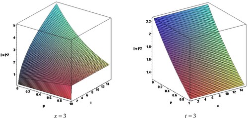
Therefore, the exact solution of the considered Equation (1) is (30) $u(x,t)=\sqrt{-\lambda -c{t}^{1-\mu }}{e}^{i(x-ct)},0<\mu \le 1.$(30) Figures 7–9 show the graph of the corresponding solutions for the proposed equation.

Figure 7. The solution (30) for $\mu =0.25,0.6,0.75$, respectively.

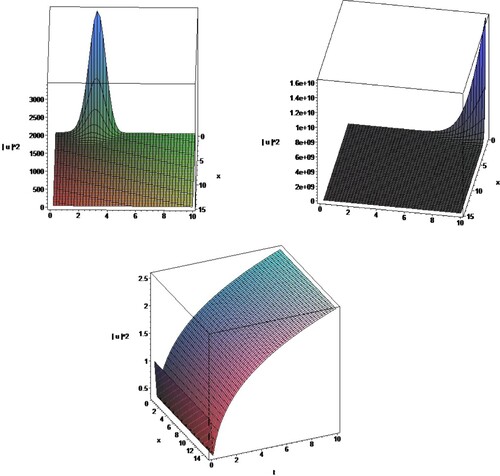
Figure 8. The solution (35) for various values of $\mu$ at $x=1$.

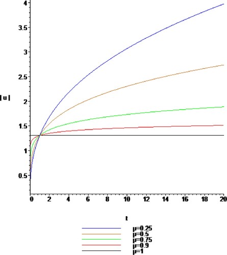
Figure 9. The solution (35) for fixed values of $x$ and $t$, respectively.

Case 2: Using the general transformation $u(x,t)=z(\xi )e^{i(\sigma (\xi )-ct)},\xi =x-mt,$the following equations are attained due to imaginary and real parts, respectively. (31) $\begin{array}{rl}& \lambda z^{\mathrm{\prime }\mathrm{\prime }\mathrm{\prime }}+({\sigma }^{\mathrm{\prime }}-m{t}^{1-\mu }+3\lambda {({\sigma }^{\mathrm{\prime }})}^2)z^{\mathrm{\prime }}\\ & +\left(\frac{1}{2}-3\lambda {\sigma }^{\mathrm{\prime }}\right){\sigma }^{\mathrm{\prime }\mathrm{\prime }}z=0,\end{array}$(31) (32) $\begin{array}{rl}& \left(\frac{1}{2}-3\lambda {\sigma }^{\mathrm{\prime }}\right)z^{\mathrm{\prime }\mathrm{\prime }}-3\lambda {\sigma }^{\mathrm{\prime }\mathrm{\prime }}{z}^{\mathrm{\prime }}\\ & +\left(c{t}^{1-\mu }+m{\sigma }^{\mathrm{\prime }}{t}^{1-\mu }-\frac{1}{2}{({\sigma }^{\mathrm{\prime }})}^2-\lambda {\sigma }^{\mathrm{\prime }\mathrm{\prime }\mathrm{\prime }}+\lambda {({\sigma }^{\mathrm{\prime }})}^3\right)z\\ & +z^3=0.\end{array}$(32) Considering $\sigma (\xi )=\frac{\xi }{6\lambda }+C_1$, the analytical solution of the first equation is (33) $\begin{array}{rl}z(\xi )& =C_2+C_3\sin \left(\frac{\xi \sqrt{-36m\lambda t^{1-\mu }+3}}{6\lambda }\right)\\ & +C_4\cos \left(\frac{\xi \sqrt{-36m\lambda t^{1-\mu }+3}}{6\lambda }\right).\end{array}$(33) Substituting the analytical solution $z(\xi )$ into the second equation, (34) $C_2=\left(\begin{array}{l}-\lambda C_3\sin \left(\frac{\zeta \sqrt{-36t^{(1-\mu )}m\lambda +3}}{6\lambda }\right)\\ -\lambda C_4\cos \left(\frac{\zeta \sqrt{-36t^{(1-\mu )}m\lambda +3}}{6\lambda }\right)\\ +\frac{1}{18}{\left(\begin{array}{l}324{\lambda }^2{C_4}^2\cos {\left(\frac{\zeta \sqrt{-36t^{(1-\mu )}m\lambda +3}}{6\lambda }\right)}^2\\ -54t^{(1-\mu )}m\lambda \\ -324t^{(1-\mu )}c{\lambda }^2+3-324{\lambda }^2{C_4}^2\\ +324{\lambda }^2{C_4}^2\sin {\left(\frac{\zeta \sqrt{-36t^{(1-\mu )}m\lambda +3}}{6\lambda }\right)}^2\end{array}\right)}^{1/2}\end{array}\right)/\lambda$(34) is obtained.

Therefore, the exact solution of the considered Equation (1) with general transformation is (35) $\begin{array}{rl}u(x,t)& =(C_2+C_3\sin \left(\frac{(x-mt)\sqrt{-36t^{(1-\mu )}m\lambda +3}}{6\lambda }\right)\\ & +C_4\sin \left(\frac{(x-mt)\sqrt{-36t^{(1-\mu )}m\lambda +3}}{6\lambda }\right))\\ & \times \exp \left(\left(\frac{x-mt}{6\lambda }+C_1-ct\right)I\right),\end{array}$(35) where $C_2$ is given above.

3. Conclusion

In this work, TEM and the direct method are considered to investigate exact solutions of the NCFSH equation. To this purpose, NCFSH equation is converted into an integer order ordinary differential equation by using the rules of the conformable derivative and the considered transformations. Using these methods, Maple and Mathematica, the optical wave solutions including various types of solitons that can be useful in nonlinear optics and telecommunication industry are obtained. Physical meanings and dynamical behaviours of the solutions are exhibited by using figures. Results indicate that these methods are powerful tools for NPDEs. Obtained solutions represent some real-life situations. Additionally, as seen in the proposed results, these suggested methods can be implemented to various fractional models arising in other areas of physics and science.

Disclosure statement

No potential conflict of interest was reported by the author(s).

References

- Baleanu D. About fractional quantization and fractional variational principles. Commun Nonlinear Sci Numer Simul. 2009;14(6):2520–2523.
- Malomed B. Nonlinear Schrödinger Equations. In: Scott A, editor. Encyclopedia of Nonlinear Science. New York: Routledge; 2005. p. 639–643.
- Laskin N. Fractional quantum mechanics and Lévy path integrals. Phys Lett A. 2000;268:298–305.
- Biswas A. Optical solitons: quasi-stationarity versus Lie transform. Opt Quantum Electron. 2003;35:979–998.
- Eslami M, Rezazadeh H, Rezazadeh M, et al. Exact solutions to the space–time fractional Schrödinger–Hirota equation and the space–time modified KDV–zakharov–Kuznetsov equation. Opt Quantum Electron. 2007;49(279).
- Kilic B, Inc M. Optical solitons for the Schrödinger–Hirota equation with power law nonlinearity by the bäcklund transformation. Optik (Stuttg). 2017;138:64–67.
- Rezazadeh H, Mirhosseini-Alizamini SM, Eslami M, et al. New optical solitons of nonlinear conformable fractional Schrödinger-Hirota equation. Optik (Stuttg). 2018;172:545–553.
- Khalil R, Horani MA, Sababheh AMY. et al. A new definition of fractional derivative. J Comput Appl Math. 2014;264:65–70.
- Abdeljawad T. On conformable fractional calculus.J Comput Appl Math. 2015;279:57–66.
- Pinar Z. On the explicit solutions of fractional Bagley–Torvik equation arises in engineering. Int J Optim Control: Theor Appl. 2019;9(3):52–58.
- Mehreen N, Anwar M. Hermite–Hadamard and Hermite–Hadamard–Fejer type inequalities for p-convex functions via new fractional conformable integral operators. J Math Computer Sci. 2019;19(4):230–240.
- Korkmaz A, Ersoy Hepson E, Hosseini K, et al. Sine-Gordon expansion method for exact solutions to conformable time fractional equations in RLW-class. J King Saud Univ Sci. 2020;32(1):567–574.
- Khalil R, Al Horani M, Abu Hammad M. Geometric meaning of conformable derivative via fractional cords. J Math Computer Sci. 2019;19(4):241–245.
- Qi Y, Wang X. Asymptotical stability analysis of conformable fractional systems. J Taibah Univ Sci. 2020;14(1):44–49.
- Md NA, Tunç C. Constructions of the optical solitons and other solitons to the conformable fractional Zakharov–Kuznetsov equation with power law nonlinearity. J Taibah Univ Sci. 2020;14(1):94–100.
- Rani M, Ahmed N, Dragomir SS, et al. Some newly explored exact solitary wave solutions to nonlinear inhomogeneous murnaghan’s rod equation of fractional order. J Taibah Univ Sci. 2021;15(1):97–110.
- Sabi’u J, Jibril A, Gadu AM. New exact solution for the (3 + 1) conformable space–time fractional modified Korteweg–de-Vries equations via sine–cosine method.J Taibah Univ Sci. 2019;13(1):91–95.
- Younis M, Rizvi STR. Dispersive dark optical soliton in (2 + 1)-dimensions by (G′/G)-expansion with dual-power law nonlinearity. Optik (Stuttg). 2015;126(24):5812–5814.
- Parkes EJ. Observations on the basic G/G'-expansion method for finding solutions to nonlinear evolution equations. Appl Math Comput. 2010;217:1759–1763.
- Wazwaz AM. Partial differential equations: methods and applications. Leiden: Balkema; 2002.
- Wazwaz AM. Partial Differential Equations and Solitary Wave Theory. Beijing and Springer-Verlag Berlin Heidelberg: Higher Education Press; 2009.
- Akbulut A, Kaplan M. Auxiliary equation method for time-fractional differential equations with conformable derivative. Comput Math with Appl. 2018;75(3):876–882.
- Vitanov NK. Modified method of simplest equation: powerful tool for obtaining exact and approximate traveling-wave solutions of nonlinear PDEs. Commun Nonlinear Sci Numer Simul. 2011;16:1176–1185.
- Yomba E. The extended fan’s sub-equation method and its application to KdV-MKdV, BKK and variant Boussinesq equations. Phys Lett A. 2005;336:463–476.
- Seadawy AR, Kumar D, Hosseini K, et al. The system of equations for the ion sound and langmuir waves and its new exact solutions. Results Phys. 2018;9:1631–1634.
- Kumar D, Kaplan M. New analytical solutions of (2 + 1)-dimensional conformable timefractional Zoomeronequation via two distinct technique. Chin J Phys. 2018;56:2173–2185.
- Liu S, Debbouche A, Wang JR. ILC method for solving approximate controllability of fractional differential equations with noninstantaneous impulses. J Comput Appl Math. 2018;339:343–355.
- Wang J, Feckan M, Zhou Y. Weakly picard operators method for modified fractional iterative functional differential equations. Fix Point Theory. 2014;15(1):297–310.
- Hosseini K. Application of the invariant subspace method in conjunction with the fractional sumudu’s transform to a nonlinear conformable timefractional dispersive equation of the fifth-order. Comput Methods Differ Equ. 2019;7(3):359–369.
- Ullah R, Ellahi R, Sait SM, et al. On the fractional-order model of HIV-1 infection of CD4+ T-cells under the influence of antiviral drug treatment. J Taibah Univ Sci. 2020;14(1):50–59.
- Ullah R, Ellahi R, Mohyud-Din ST, et al. Exact traveling wave solutions of fractional order boussinesq-like equations by applying Exp-function method. Results Phys. 2018;8:114–120.
- Liu CS. A new trial equation method and its applications. Commun Theor Phys. 2006;45(3):395–397.
- Liu CS. Trial equation method to nonlinear evolution equations with rank inhomogeneous: mathematical discussions and its applications. Commun Theor Phys. 2006;45(2):219–223.
- Odabasi M. Traveling wave solutions of conformable time-fractional Zakharov–Kuznetsov and Zoomeron equations. Chin J Phys. 2020;64:194–202.
- Odabasi M, Pinar Z, Kocak H. Analytical solutions of some nonlinear fractional-order differential equations by different methods. Math Methods Appl Sci. 2021;44:7526–7537.
- Pinar Z, Koprulu M O, Kocak H. Symbolic computations for exact solutions of fractional partial differential equations with reaction term. Submitted, 2021.