
 ?Mathematical formulae have been encoded as MathML and are displayed in this HTML version using MathJax in order to improve their display. Uncheck the box to turn MathJax off. This feature requires Javascript. Click on a formula to zoom.
Abstract
This paper seeks to estimate the entropy for the inverse Weibull distribution using progressively Type-II censored data. To reach this objective, the entropy is defined through three entropy measures, namely, Rényi, q-entropy and Shannon entropy, and two estimation methods are used to estimate them. The first approach to estimate these quantities is the method of maximum likelihood. Furthermore, and for the first time, we consider the method of maximum product of spacing to estimate the mentioned entropy measures. Also, a simulation study is carried out and two real data sets are analysed. The numerical outcomes showed that the maximum likelihood provides good point estimates while the interval estimates based on the maximum product of spacing method have the shortest confidence interval lengths.
1. Introduction
Entropy is the expected quantity of information for the random variable. Measuring entropy is a very important role in many areas such as statistics, physics, chemicals, economics, insurance, financial analysis and biological phenomenon. More entropy is referred to less information found in a sample. Using the approaches of probability and statistics, the concept of entropy was defined by [Citation1] as a measure of information. This concept was enhanced by numerous other entropy measures, arising from different real applications, see for complete survey [Citation2]. In this study, we focus our attention on three of the most popular entropy measures, namely, Rényi entropy (RE) by [Citation3], the q-entropy (QE) by [Citation4] and Shannon entropy (SE) by [Citation1].
Let X be a random variable with a probability density function (PDF) , where Ω is the vector of the unknown parameters. Then, the RE, QE and SE of X are defined, respectively, as follow
(1)
(1)
(2)
(2) and
(3)
(3) In most of the studies, at least Ω is unknown as well as the entropy. For this reason, estimating the parameters and the entropy has been the object of all the attention in various studies. See for example [Citation5–13].
The inverse Weibull (IW) distribution occupies an essential place in representing the lifetime of components and investigating different extreme circumstances retaining rainfall, sea waves, wind speeds, earthquakes, floods queues in supermarkets, etc. The IW distribution furnishes a useful fit for non-monotone failure rates, such as decreasing and unimodal failure rates. The random variable X has the two-parameter IW distribution, denoted by IW, if its PDF and cumulative distribution function (CDF), are respectively, given as
(4)
(4) and
(5)
(5) where
is the shape parameter and
is the scale parameter.
This study gives a contribution to the estimation of the RE, QE and SE for the IW distribution based on progressive Type-II censoring (PT-IIC) data. We first use the maximum likelihood (ML) estimation method to estimate the entropy measures based on the invariance property of the ML method. The approximate confidence intervals (ACIs) for these quantities are also obtained. Besides this approach and for the first time, we consider using the maximum product of spacing (MPS) estimation method to estimate the entropy measures and to construct the corresponding ACIs. To compare the performance of the different estimates, a simulation study is implemented. Finally, to show the applicability of the proposed methods, two real data sets are investigated.
The rest of this paper is organized as follows: The expressions of the three entropy measures are derived in Section 2. The ML method is investigated in Section 3. In Section 4, the estimates of the entropy measures are obtained using the MPS approach. A simulation study is conducted in Section 5, and two real data sets are studied in Section 6. Lastly, the paper is concluded in Section 7.
2. Expressions of entropies
Let X be a random variable following the IW distribution, then, using (Equation1(1)
(1) ) and (Equation4
(4)
(4) ) with
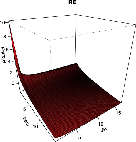
, the RE of X can be written as
(6)
(6) with
,
and
. Figure displays the plot of the RE for the IW distribution for different values of β and ζ with
. Figure shows that the RE of the IW distribution is decreasing as β and ζ increase.
Figure 1. Plot of the RE for the IW distribution.
Similarly, the QE of the random variable X can be obtained based on (Equation2(2)
(2) ) and (Equation4
(4)
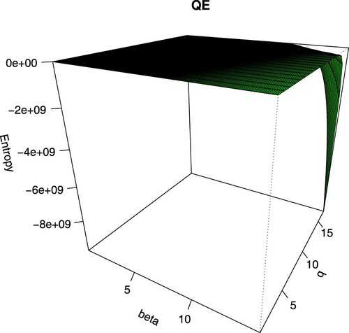
(4) ) as
(7)
(7) with
,
and
. Figure shows the plot of the QE for the IW distribution for different values of β and q with
. It is noted from Figure that as β and q increase, the QE of the IW distribution decreases.
Figure 2. Plot of the QE for the IW distribution.
Also, the SE of a random variable X can be obtained from (Equation3(3)
(3) ) and (Equation4
(4)
(4) ) as
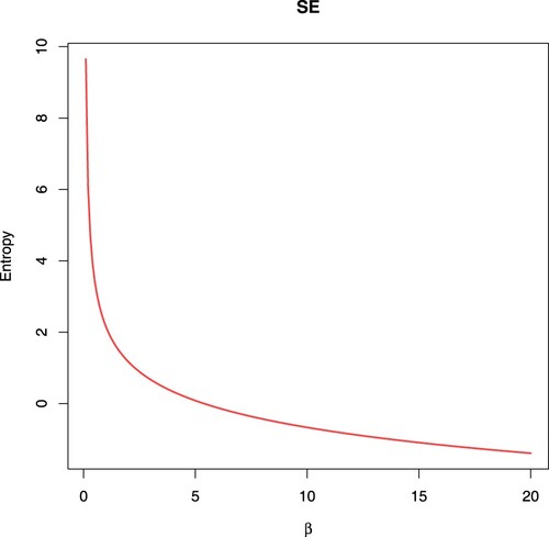
After some simplifications, the SE of IW model is given by
(8)
(8) where γ is Euler constant. Figure depicts the plot of the SE for the IW distribution for different values of β with
, which indicates that the SE is decreasing as β increases.
Figure 3. Plot of the SE for the IW distribution.
3. Estimation of entropies using ML method
In this section, the ML method is used to obtain the point and interval estimates of the unknown parameters of the IW distribution as well as the entropy measures based on a PT-IIC sample.
3.1. ML estimation
Due to rapid advancements in technology, researchers often want to save costs and the total time on the test. Therefore, a general censoring scheme called PT-IIC scheme can be considered. In the PT-IIC scheme, n items are put on a life test with a predetermined censoring scheme , where m is the effective sample size. For more details about PT-IIC scheme, see for example [Citation14–16]. See also for more details [Citation17–19]. Let
be a PT-IIC sample of size m with progressive censoring scheme
. Then, the likelihood function (LF), ignoring the constant term, can be written as
(9)
(9) From (Equation4
(4)
(4) ), (Equation5
(5)
(5) ) and (Equation9
(9)
(9) ), the natural logarithm of the LF,
, can be given as
(10)
(10) The first partial derivatives of (Equation10
(10)
(10) ) with respect to α and β are given, respectively, by
(11)
(11) and
(12)
(12) The maximum likelihood estimates (MLEs) of β and α denoted by
and
can be computed by equating (Equation11
(11)
(11) ) and (Equation12
(12)
(12) ) to zero and solve the two normal equations simultaneously. Now, based on the invariance property of the MLEs, the MLEs of the entropies
,
and
for the IW distribution can be obtained directly from (Equation6
(6)
(6) ), (Equation7
(7)
(7) ) and (Equation8
(8)
(8) ), respectively, as follow
with
,
and
,
with
,
and
, and
3.2. ACIs using MLEs
To construct the ACIs of the entropy measures ,
and
, we should first obtain the approximate asymptotic variance-covariance (VC) matrix of the MLEs. In this case, the approximate asymptotic VC can be computed through the inverse of the observed Fisher information matrix as follows
(13)
(13) The elements of (Equation13
(13)
(13) ) are given by
and
Here, we employ the delta method to get the approximate variances of the entropy measures. Let
,
and
, which are obtained at the MLEs of α and β, where
(14)
(14)
(15)
(15) and
(16)
(16) where
gives the digamma function,
is the ordinary derivative of
and
. Now, the approximate estimates for the variances of the entropy measures
,
and
can be obtained, respectively, as
Therefore, the two-sided ACIs for
,
and
at confidence level
, are given, respectively, by
where
is the
standard normal percentile.
4. Estimation of entropies using MPS method
Cheng and Amin [Citation20] introduced the MPS method and many other authors used this method because the MPS estimators (MPSEs) retain most of the properties of the MLEs including the invariance property, see [Citation21,Citation22]. For more details about the MPS method, one can refer to [Citation23–26]. Based on a PT-IIC sample, the MPS function can be written according to [Citation27] as follows
(17)
(17)
4.1. MPS estimation
The MPS function of the IW distribution can be obtained from (Equation4(4)
(4) ), (Equation5
(5)
(5) ) and (Equation17
(17)
(17) ) as follows
(18)
(18) The natural logarithm of (Equation18
(18)
(18) ), denoted by
, takes the form
(19)
(19) The MPSEs of α and β, denoted by
and
, respectively, are obtained by solving the following normal equations simultaneously
(20)
(20) and
(21)
(21) Any numerical method can be implemented to get
and
from (Equation20
(20)
(20) ) and (Equation21
(21)
(21) ), respectively. Utilizing the invariance property of the MPSEs, the MPSEs of the entropies
,
and
can be acquired from (Equation6
(6)
(6) ), (Equation7
(7)
(7) ) and (Equation8
(8)
(8) ), respectively, as
with
,
and
,
with
,
and
, and
4.2. ACIs using MPSEs
In order to construct the ACIs of ,
and
, we first obtain the approximate asymptotic VC matrix based on the MPSEs as follows
(22)
(22) The second derivatives of the (Equation19
(19)
(19) ) with respect to α and β are given by
and
where
and
Now, we use the delta method to approximate the variances of
,
and
. We first obtain the quantities
and
, where the elements of these quantities are given by (Equation14
(14)
(14) )–(Equation16
(16)
(16) ). Therefore, the approximates variances of
,
and
can be computed, respectively, as
Several authors have elicited the asymptotic equivalence of the MPS and ML methods, Refs. [Citation20,Citation22,Citation28] revealed that the MPS method also exhibits asymptotic properties like the ML method. One can also refer to [Citation29]. Therefore, the two-sided ACIs for
,
and
at confidence level
, are given, respectively, by
5. Monte Carlo simulation
To investigate the behaviour of ,
and
, an extensive Monte Carlo simulation study is conducted. Using different combinations of n, m and
, we generate 1,000 PT-IIC samples under two sets of the true value of
such as
(Set-1) and
(Set-2). Further, to estimate
and
, two different choices of ζ and q are used namely,
and
. The true values of
and
based on Set-1 and 2 are
,
,
and
, respectively. Also, three censoring schemes (Schs) are also considered as
For each setting, the root mean square errors (RMSEs) and relative absolute biases (RABs) are computed for each entropy measure and reported in Tables and . Also, the confidence lengths (CLs) as well as the coverage probabilities (CPs) of these measures are also obtained and presented in Tables and . We refer to the RE entropy as
and to QE as
in the simulation and real data outcomes. All numerical computations are implemented via “maxLik” package, proposed by [Citation30], in the
statistical programming language software which using Newton-Raphson method of maximization in the computations.
Table 1. Average RMSEs and RABs (in parentheses) of ,
and
for
.
Table 2. Average RMSEs and RABs (in parentheses) of ,
and
for
.
Table 3. The ACLs of ,
and
with their CPs in parentheses, when
.
Table 4. The ACLs of ,
and
with their CPs in parentheses, when
.
For the parameter estimation, the outcomes of the simulation study showed that the ML approach provides better estimates than the MPS approach in terms of minimum RMSEs and RABs. On the other hand, the MPS approach gives more accurate interval estimates in terms of minimum ACLs. From the simulation results established in Tables , in respect of RMSEs, RABs, ACLs and CPs of the proposed estimates, we can obtain the following considerations. In general, it can be seen that the MLEs and MPSEs of ,
and
are very good in terms of minimum RMSEs, RABs and ACLs as well as highest CPs. As n (or
) increases, the RMSEs, RABs and ACLs of all investigated estimates decrease while CPs increase as expected. Therefore, to get better estimation results, one may tend to increase the total (or effective) sample size. As α and β increase, the RMSEs associated with all proposed estimates decrease while the RABs increase. In most cases, when α and β increase, it is observed that the ACLs constructed based on LF and MPS approaches decrease while the corresponding CPs increase. Further, for each setting, it is evident that the RMSEs associated with MLEs decrease for both
and
when ζ and q increase. Similar behaviour is observed in the case of MPSEs of
and
. As ζ increases, the corresponding RABs of all estimates increase when
. Also, as q increases, the corresponding RABs of all estimates increase when
while these decrease when
. In addition, for each test, ζ and q increase, the CPs using both LF and MPS approaches are mostly below (or near to) the specified nominal level.
Comparing the proposed censoring schemes I, II and III, it is observed that the MLEs (based on Scheme-I) and MPSEs (based on Scheme-III) performed better than other censoring schemes in terms of the lowest RMSEs and RABs for both true value sets. Also, the interval estimates, using observed likelihood samples, performed better based on Scheme-III compared to the other censoring schemes in terms of the shortest ACLs and highest CPs. It is also noted that the ACI estimates using the MPS approach worked effectively based on censoring schemes I and II when taken as
and
, respectively. To sum up, simulation results showed that the likelihood approach has performed superior to the other in the case of point estimation while the product of spacings approach has performed superior to the other in the case of interval estimation.
6. Real-life applications
To show the adaptability and flexibility of the proposed methodologies to a real phenomenon, we shall provide two numerical applications using real-life data sets in this section. The first data set (referred to as Data-I) represents the vinyl chloride data (in mg/L) obtained from clean-up-gradient monitoring wells. The data was first used by [Citation31] and recently analysed by [Citation32]. The second data set (referred to as Data-II) shows the times (in min) to breakdown of an insulating fluid between 19 electrodes recorded at 34 kV. The Data-II was reported by [Citation33] and recently analysed by [Citation34,Citation35]. The ordered values of Data-I and -II are presented in Table .
Table 5. The real data sets.
We first fit the IW distribution to the two data sets. For this purpose, the Kolmogorov-Smirnov (K-S) and Cramér-von Mises (CvM) goodness-of-fit test statistics with associated p-values are reported in Table . The MLEs and the corresponding standard errors (SErs) and the goodness of fit statistics are displayed in Table , which show that the IW distribution is a suitable model to fit the two data set.
Table 6. MLEs (with SEs in parentheses) and goodness of fit statistics for the real data.
Now, from Table , three PT-IIC samples are generated using different choices of m and R. These generated samples are provided in Table . In short, the censoring scheme is referred as
. Using the generated sample, the MLEs and MPSEs of the unknown parameters as well as
,
and
with their SErs are reported in Table for the two data sets. Also, the 95% ACIs of these quantities with their lengths are listed in Table . From Tables and , it is observed that the estimates of
,
and
using the MPS approach performed better than those using the ML approach in terms of minimum SErs and confidence lengths. The data analysis shows that based on the MLEs, Sch-III performs better than other schemes. The estimated entropies have the smallest values in this case, which indicates that the data obtained using Sch-III provides more information than other schemes. On the other hand, using the MPSEs, we can observe that the data acquired employing Sch-I gives more information than other schemes. Based on these results and when using the PT-IIC data, one can estimate the entropy to decide which scheme gives more information.
7. Conclusion
This article considers the estimation of the Rényi, q-entropy and Shannon entropy for inverse Weibull distribution based on progressively Type-II censored data. The methods of maximum likelihood and maximum product of spacing are used. The point estimators are acquired through the invariance property and the approximate confidence intervals are also computed. To examine the efficiency of the offered estimators, a simulation study and two real data sets are investigated. The numerical analysis shows that the maximum likelihood provides an acceptable approach to estimate the entropy measures and the maximum product of spacing is a good choice when the researcher wishes to obtain confidence intervals for these measures. For future work, the Bayesian approach can be considered to estimate the entropy measures employing both maximum likelihood and maximum product of spacing methods. Another future work is to perform the bootstrap confidence intervals of the entropies using the both estimation methods.
Table 7. Different generated PT-IIC samples.
Table 8. The MLEs and MPSEs (with their SEs in parentheses) for the real data.
Table 9. The ACIs (with confidence lengths in parentheses) for the real data.
Acknowledgements
The authors would like to express their appreciation to the editor and anonymous referees for valuable guidance and useful comments.
Disclosure statement
No potential conflict of interest was reported by the authors.
Additional information
Funding
References
- Amigó JM, Balogh SG, Hernández S. A brief review of generalized entropies. Entropy. 2018;20(11):813.
- Rényi A. On measures of entropy and information. In: Proceedings of the Fourth Berkeley Symposium on Mathematical Statistics and Probability, Volume 1: Contributions to the Theory of Statistics. University of California Press; 1961.
- Tsallis C. Possible generalization of Boltzmann-Gibbs statistics. J Stat Phys. 1988;52(1):479–487.
- Shannon CE. A mathematical theory of communication. Bell Syst Tech J. 1948;27(3):379–423.
- Wong KM, Chen S. The entropy of ordered sequences and order statistics. IEEE Trans Inform Theory. 1990;36(2):276–284.
- Baratpour S, Ahmadi J, Arghami NR. Entropy properties of record statistics. Statist Papers. 2007;48(2):197–213.
- Morabbi H, Razmkhah M. Entropy of hybrid censoring schemes. J Stat Res. 2010;6(2):161–176.
- Abo-Eleneen ZA. The entropy of progressively censored samples. Entropy. 2011;13(2):437–449.
- Cramer E, Bagh C. Minimum and maximum information censoring plans in progressive censoring. Commun Stat Theory Methods. 2011;40(14):2511–2527.
- Cho Y, Sun H, Lee K. An estimation of the entropy for a Rayleigh distribution based on doubly-generalized type-II hybrid censored samples. Entropy. 2014;16(7):3655–3669.
- Lee K. Estimation of entropy of the inverse Weibull distribution under generalized progressive hybrid censored data. J Korean Data Inform Sci Soc. 2017;28(3):659–668.
- Hassan AS, Zaky AN. Estimation of entropy for inverse Weibull distribution under multiple censored data. J Taibah Univ Sci. 2019;13(1):331–337.
- Bantan RA, Elgarhy M, Chesneau C, et al. Estimation of entropy for inverse Lomax distribution under multiple censored data. Entropy. 2020;22(6):601.
- Rastogi MK, Tripathi YM, Wu SJ. Estimating the parameters of a bathtub-shaped distribution under progressive type-II censoring. J Appl Stat. 2012;39(11):2389–2411.
- Ahmed EA. Bayesian estimation based on progressive type-II censoring from two-parameter bathtub-shaped lifetime model: an Markov chain Monte Carlo approach. J Appl Stat. 2014;41(4):752–768.
- Dey S, Nassar M, Maurya K, et al. Estimation and prediction of Marshall-Olkin extended exponential distribution under progressively type-II censored data. J Stat Comput Simul. 2018;88(2):2287–2308.
- Balakrishnan N, Aggarwala R. Progressive censoring: theory methods, and applications. Boston (MA): Birkhauser; 2000.
- Dey S, Nassar M, Kumar D. Moments and estimation of reduced Kies distribution based on progressive type-II right censored order statistics. Hacettepe J Math Stat. 2019;48(1):332–350.
- Kumar D, Nassar M, Malik MR, et al. Estimation of the location and scale parameters of generalized Pareto distribution based on progressively type-II censored order statistics. Ann Data Sci. 2020;1–35.
- Cheng RCH, Amin NAK. Estimating parameters in continuous univariate distributions with a shifted origin. J R Stat Soc Ser B. 1983;45(3):394–403.
- Coolen FPA, Newby MJ. A note on the use of the product of spacings in Bayesian inference. Department of Mathematics and Computing Science, University of Technology; 1990.
- Anatolyev S, Kosenok G. An alternative to maximum likelihood based on spacings. Econom Theory. 2005;21(2):472–476.
- Nassar M, Afify AZ, Dey S, et al. A new extension of Weibull distribution: properties and different methods of estimation. J Comput Appl Math. 2018;336:439–457.
- Shafqat M, Ali S, Shah I, et al. Univariate discrete Nadarajah and Haghighi distribution: properties and different methods of estimation. Statistica. 2020;80(3):301–330.
- Ali S, Dey S, Tahir MH, et al. Comparison of different methods of estimation for the flexible Weibull distribution. Commun Faculty Sci Univ Ankara Ser A1 Math Stat. 2020;69(1):794–814.
- Ali S, Dey S, Tahir MH, et al. The Poisson Nadarajah-Haghighi distribution: different methods of estimation. J Reliab Stat Stud. 2021;14(2):415–450.
- Ng HKT, Luo L, Hu Y, et al. Parameter estimation of three-parameter Weibull distribution based on progressively type-II censored samples. J Stat Comput Simul. 2012;82(11):1661–1678.
- Ghosh K, Jammalamadaka SR. A general estimation method using spacings. J Stat Plan Inference. 2001;93(1-2):71–82.
- Basu S, Singh SK, Singh U. Estimation of inverse Lindley distribution using product of spacings function for hybrid censored data. Methodol Comput Appl Probab. 2019;21(4):1377–1394.
- Henningsen A, Toomet O. maxLik: a package for maximum likelihood estimation in R. Comput Stat. 2011;26(3):443–458.
- Bhaumik D, Kapur K, Gibbons R. Testing parameters of a gamma distribution for small samples. Technometrics. 2009;51(3):326–334.
- Vishwakarma PK, Kaushik A, Pandey A, et al. Bayesian estimation for inverse Weibull distribution under progressive type-II censored data with beta-binomial removals. Austrian J Stat. 2018;47(1):77–94.
- Lawless JF. Statistical models and methods for lifetime data. 2nd ed. New Jersey: Wiley; 2011.
- Dey S, Nassar M. Classical methods of estimation on constant stress accelerated life tests under exponentiated Lindley distribution. J Appl Stat. 2020;47(6):975–996.
- Elshahhat A, Rastogi MK. Estimation of parameters of life for an inverted Nadarajah–Haghighi distribution from type-II progressively censored samples. J Indian Soc Probab Stat. 2021;22(1):113–154.