Rate of complete second-order moment convergence and theoretical applications

ABSTRACT

The purpose of this work is to present a novel mode of convergence, complete second-order moment convergence with rate, which implies almost complete convergence and gives a smaller rate of convergence. Indeed, this mode is easier to obtain and gives better performances than those of the almost complete convergence in the case of the nonparametric estimators with kernels of the density function, of the distribution function and of the quantile  function. A great advantage of the proposed approach is that less conditions are imposed to the kernel function thanks to the use of the mean squared error expression.

KEYWORDS:

• Kernel density estimator
• kernel distribution estimator
• kernel quantile estimator
• complete moment convergence
• nonparametric estimation
• rate of convergence
• complete convergence

1. Introduction

The rate of convergence is an important concept that describes the speed with which a sequence converges to the limit. In this setting, a fundamental question is how fast the convergence is illuminating theoretical studies on the subject has been carried out proposing important new results, algorithms and applications to address this issue. The purpose of this work is to present a novel mode of convergence, namely the complete secondorder convergence with a rate. The novelty here is in the introduction of the complete secondorder convergence rate. Hence, we give proofs of different proprieties of this kind of convergence. The almost complete convergence is induced by second-order convergence in different context (see [1–3] and recently see Yu et al. [29]). The complete convergence concept was introduced by Hsu and Robbins [4]. Then, it has been used by several authors such as Gut and Stadtmller [5], Gut [6,7], Li et al. [8], Sung [9], Sung and Volodin [10]. The interest of such a notion lies in the fact that almost complete convergence (a.c.) implies almost sure convergence (a.s.) due to the Borel–Cantelli lemma. However in some situations at least, it is much easier to obtain complete second-order moment convergence (c.s.m.) instead of almost complete convergence.

As a practical framework, rates of complete second-order moment convergence for the probability density , the distribution function and the quantile function kernel estimators are established. We also discuss about the speed at which these estimators converge. First, in the context of estimating probability density function, many studies using different methods have been proposed. The Kernel method is one of the best of these methods which seems to be convenient and does not require a multiple choice of parameters. Rosenblatt [11] was the earliest pioneer of the class of kernel density estimators, using two parameters, namely the kernel and the bandwidth. For this estimator, convergence in probability was established by Parzen [12]. Habbema et al. [13], Hall and Kang [14], Hall and Wand [15], Gosh and Chaudhury [16] and Gosh and Hall [17] can be consulted for various works on the subject, in particular the estimation by classical kernels of the densities. In the case of independent observations, optimal rates of convergence to zero for mean square error and the bias of the kernel estimators have been addressed by several authors under varying conditions on the kernel (K) and the density (f ). As a contribution, a new complete second-order moment convergence with a rate is introduced for the first time to improve the rates of convergence for the bias and the mean square error (MSE) of kernel density estimators. Then the complete convergence of the density kernel estimator, under weaker conditions on the density function than those proposed in the literature, is achieved. As a consequence of the complete second-order moment convergence, the almost complete convergence is obtained with a better rate.

Second, the proposed mode of convergence is applied to the distribution function and quantiles kernel estimators. Notice that for the distribution function, Nadaraya [18] proposed its kernel estimator. While, Parzen [19] retraced the context of Nadaraya [18] and constructed the kernel quantile estimators for which we established the rate of almost complete convergence. To the best of our knowledge, this is a new result obtained from the proposed convergence mode. A great advantage of the proposed approach is that less conditions are imposed to the kernel function thanks to the use of the mean squared error expression.

2. Complete second-order moment convergence with a rate

Throughout this paper, real-valued random variables are defined on a fixed probability space $(\mathrm{\Omega },\mathcal{A},P)$.

Let $(U_n{)}_{n\in \mathbb{N}}$ and $(V_n{)}_{n\in \mathbb{N}}$ be two sequences of real numbers. We assume $(V_n{)}_{n\in \mathbb{N}}$ does not vanish from a certain rank. We say that $(U_n{)}_{n\in \mathbb{N}}$ is dominated by $(V_n{)}_{n\in \mathbb{N}}$ if there exist a real number M and an integer $n_0$, such that, for all $n\ge n_0$, we have $|U_n|\le M|V_n|,$and we note $U_n=O\left(V_n\right)$.

Definition 2.1

A sequence $(X_n{)}_{n\in \mathbb{N}}$ of random variables is said to be almost complete second-order moment convergent (c.s.m) to the random variable X, with the convergence rate $\frac{1}{\sqrt{U_n}}$, if $\sum _{n\in \mathbb{N}}^{}{U}_{n}E(X_n-X{)}^2<\mathrm{\infty },$where $\left(U_n\right)$ in a sequence of positive numbers. Note this mode $X_n-X=O_{c.s.m}\left(\frac{1}{\sqrt{U_n}}\right).$

The following theorem shows that if $(X_n{)}_{n\in \mathbb{N}}$ converges in complete second-order moment to X with a rate $\frac{1}{\sqrt{U_n}}$, then it is almost completely convergent with a rate of $\frac{1}{\sqrt{U_n}}.$

Theorem 2.1

If a sequence $(X_n{)}_{n\in \mathbb{N}}$ of random variables verifies $X_n-X=O_{c.s.m}\left(\frac{1}{\sqrt{U_n}}\right),$then $X_n-X=O_{a.c}\left(\frac{1}{\sqrt{U_n}}\right).$And for $\text{β}>-1$, $ϵ>0$ and the sequence $(V_n{)}_{n\in \mathbb{N}}=(n^{\text{β}}{U}_n{)}_{n\mathbb{N}}$ we obtain $\sum _{n\in \mathbb{N}}^{}{n}^{\text{β}}P(|X_n-X|>ϵ)\le \sum _{n\in \mathbb{N}}^{}{n}^{\text{β}}{U}_{n}E(X_n-X{)}^2<\mathrm{\infty }.$

Proof.

Suppose that $\sum _{n\in \mathbb{N}}^{}{U}_{n}E(X_n-X{)}^2<\mathrm{\infty },$ then from the Markov inequality we obtain $P(|X_n-X|\ge \frac{1}{\sqrt{U_n}})\le U_{n}E(X_n-X{)}^2,$so $\sum _{n\in \mathbb{N}}^{}P(|X_n-X|\ge \frac{1}{\sqrt{U_n}})\le \sum _{n\in \mathbb{N}}^{}{U}_{n}E(X_n-X{)}^2<\mathrm{\infty }.$Now, $\frac{1}{\sqrt{U_n}}$ is a rate of convergence, so $\frac{1}{\sqrt{U_n}}⟶0$ which equivalent to, for each $ϵ>0$, there exist $n_0\in \mathbb{N}$ such that for all $n\ge n_0$ we have $\frac{1}{\sqrt{U_n}}<ϵ$. So $P(|X_n-X|>ϵ)\le P(|X_n-X|\ge \frac{1}{\sqrt{U_n}})$which implies $\sum _{n\in \mathbb{N}}^{}{n}^{\text{β}}P(|X_n-X|>ϵ)\le \sum _{n\in \mathbb{N}}^{}{n}^{\text{β}}{U}_{n}E(X_n-X{)}^2<\mathrm{\infty }.$

The following proposition gives some elementary calculus rules.

Proposition 2.1

Assume $\underset{n⟶\mathrm{\infty }}{lim}{U}_n=+\mathrm{\infty },X_n-l_X=O_{c.s.m}\left(\frac{1}{\sqrt{U_n}}\right)$ and $Y_n-l_Y=O_{c.s.m}\left(\frac{1}{\sqrt{U_n}}\right),$ where $l_X,l_Y$ are real numbers. We have

(1)	$(X_n+Y_n)-(l_X+l_Y)=O_{c.s.m}\left(\frac{1}{\sqrt{U_n}}\right)$;
(2)	$X_n.Y_n-l_X.l_Y=O_{c.s.m}\left(\frac{1}{\sqrt{U_n}}\right)$;
(3)	$\frac{1}{X_n}-\frac{1}{l_X}=O_{c.s.m}\left(\frac{1}{\sqrt{U_n}}\right),$ with $l_X\ne 0$.

Proof.

1. Immediately from the following inequality: $\begin{array}{rl}& \sum _{n\in \mathbb{N}}^{}{U}_{n}E\left(\right(X_n+Y_n)-(l_X+l_Y){)}^2\\ & \le 2^2\left(\sum _{n\in \mathbb{N}}^{}{U}_{n}E\right(X_n-l_X{)}^2+\sum _{n\in \mathbb{N}}^{}{U}_{n}E(Y_n-l_Y{)}^2).\end{array}$

2. We have $\begin{array}{rl}& E(X_n.Y_n-l_X.l_Y{)}^2\\ & ={\int }_0^{+\mathrm{\infty }}P(|X_n.Y_n-l_X.l_Y|>\sqrt{t})\mathrm{d}t\\ & ={\int }_0^{+\mathrm{\infty }}P\left(|\right(X_n-l_X\left)\right(Y_n-l_Y)+l_Y(X_n-l_X)\\ & +l_X(Y_n-l_Y)|>\sqrt{t})\mathrm{d}t\\ & \le E|X_n-l_X{|}^2+E|Y_n-l_Y{|}^2\\ & +l_Y^{2}E|X_n-l_X{|}^2+l_X^{2}E|Y_n-l_Y{|}^2,\end{array}$then $\begin{array}{rl}& \sum _{n\in \mathbb{N}}^{}{U}_{n}E(X_n.Y_n-l_X.l_Y{)}^2\\ & \le \sum _{n\in \mathbb{N}}^{}{U}_{n}E|X_n-l_X{|}^2+\sum _{n\in \mathbb{N}}^{}{U}_{n}E|Y_n-l_Y{|}^2\\ & +\sum _{n\in \mathbb{N}}^{}{U}_n{l}_Y^{2}E|X_n-l_X{|}^2+\sum _{n\in \mathbb{N}}^{}{U}_n{l}_X^{2}E|Y_n-l_Y{|}^2\\ & <\mathrm{\infty }.\end{array}$

3. For $l_X\ne 0$ $\begin{array}{rl}E{(\frac{1}{X_n}-\frac{1}{l_X})}^2& ={\int }_0^{+\mathrm{\infty }}P(|\frac{1}{X_n}-\frac{1}{l_X}{|}^2>t)\mathrm{d}t\\ & ={\int }_0^{+\mathrm{\infty }}P(|X_n-l_X{|}^2>t.(X_n.l_X{)}^2)\mathrm{d}t\\ & \le {\int }_0^{+\mathrm{\infty }}P(|X_n-l_X{|}^2>t)\mathrm{d}t\\ & \le E|X_n-X{|}^2,\end{array}$so $\sum _{n\in \mathbb{N}}^{}{U}_{n}E{(\frac{1}{X_n}-\frac{1}{l_X})}^2\le \sum _{n\in \mathbb{N}}^{}{U}_{n}E|X_n-X{|}^2<\mathrm{\infty }.$

Now we have two properties which are consequences of the previous calculus rules.

Corollary 2.1

Assume $\underset{n⟶\mathrm{\infty }}{lim}{U}_n=+\mathrm{\infty }$, $X_n=O_{c.s.m}\left(\frac{1}{\sqrt{U_n}}\right)$ and $Y_n=O_{c.s.m}\left(\frac{1}{\sqrt{U_n}}\right),$ where $l_Y$ is a reel number. We have

(1)	$(X_n.Y_n)=O_{c.s.m}\left(\frac{1}{\sqrt{U_n}}\right)$;
(2)	$\frac{X_n}{Y_n}=O_{c.s.m}\left(\frac{1}{\sqrt{U_n}}\right),$ with $l_X\ne 0.$

Proof.

Follows directly from Proposition 2.1.

3. Theoretical applications

In this section, rates of complete second-order moment convergence for the probability density , the distribution function and the quantile function  kernel estimators are established. The following remark is very important to establish these rates.

Remark 3.1

In all that follows, the supposition of the convergence of $\sum _{n\ge 1}{U}_n{h}_n^4$ or $\sum _{n\ge 1}\frac{U_n}{h_n^2}$ follows from the fact that, if $h_n<1$ we have $U_n{h}_n^4\le \frac{U_n}{h_n^2}$, so the convergence of $\sum _{n\ge 1}\frac{U_n}{h_n^2}$ implies the convergence of $\sum _{n\ge 1}{U}_n{h}_n^4$. If $h_n>1$ and $h_n⟶0$ while $n⟶\mathrm{\infty }$, the convergence is obtained.

3.1. Kernel density estimator

Let $X_1$, $X_2$,…, $X_n$ be independent and identically distributed copies of a random variable X, which has unknown continuous probability density function f. The kernel density estimator, noted $\widehat{f_n}$, of the unknown density f defined by Parsen [12]; Rosenblatt [11], is given by $\widehat{f_n}\left(x\right)=\frac{1}{n{h}_n}\sum _{i=1}^{n}K\left(\frac{x-X_i}{h_n}\right),$where $(h_n{)}_{n\ge 1}$ is a sequence of positive numbers, usually called a bandwidth or smoothing parameter, and K is an integrable Borel measurable function satisfying $K\ge 0$ and ${\int }_{\mathbb{R}}K\left(x\right)\mathrm{d}x=1$, called kernel. Assume that the kernel K and the density f functions verify the following conditions:

(H1)	$\mathrm{\forall }x\in \mathbb{R}$, $K\left(x\right)=K(-x)$;
(H2)	$\underset{x\in \mathbb{R}}{sup}\mid K\left(x\right)\mid \le M<\mathrm{\infty }$;
(H3)	${\int }_{-\mathrm{\infty }}^{+\mathrm{\infty }}{x}^{2}K\left(x\right)\mathrm{d}x<\mathrm{\infty }$;
(H4)	$f\in C^2$ and $f^{\left(2\right)}$ is bounded.

Theorem 3.1

Under (H1)–(H4) and supposing that $\sum _{n\ge 1}{U}_n{h}_n^4$ or $\sum _{n\ge 1}\frac{U_n}{h_n^2}$ converges (see Remark 3.1), we have (1) $\widehat{f_n}\left(x\right)-f\left(x\right)=O_{c.s.m}\left(\frac{1}{\sqrt{U_n}}\right),$(1)

Proof.

To prove (1(1) $\widehat{f_n}\left(x\right)-f\left(x\right)=O_{c.s.m}\left(\frac{1}{\sqrt{U_n}}\right),$(1) ), notice first that the mean squared error MSE of $\widehat{f_n}$, defined by $MSE\left(\widehat{f_n}\right(x\left)\right)=E\left(\widehat{f_n}\right(x)-f(x){)}^2,$can be written as (2) $MSE\left(\widehat{f_n}\right(x\left)\right)=Bias\left(\widehat{f_n}\right(x){)}^2+Var(\widehat{f_n}\left(x\right)).$(2) Hence to prove (1(1) $\widehat{f_n}\left(x\right)-f\left(x\right)=O_{c.s.m}\left(\frac{1}{\sqrt{U_n}}\right),$(1) ), it suffices to show that (3) $\sum _{n\ge 1}{U}_{n}Var\left[\widehat{f_n}\right(x\left)\right]<\mathrm{\infty }$(3) and (4) $\sum _{n\ge 1}{U}_{n}Bias\left(\widehat{f_n}\right(x){)}^2<\mathrm{\infty }.$(4) For the inequality (3(3) $\sum _{n\ge 1}{U}_{n}Var\left[\widehat{f_n}\right(x\left)\right]<\mathrm{\infty }$(3) ) $\begin{array}{rl}Var\left[\widehat{f_n}\right(x\left)\right]& =\frac{1}{n^2{h}_n^2}Var\sum _{i=1}^{n}K\left(\frac{x-X_i}{h_n}\right)\\ & \le \frac{1}{n{h}_n^2}E\left[K^2\left(\frac{x-X}{h_n}\right)\right].\end{array}$Using the condition (H2) of the kernel K, it follows that $Var\left[\widehat{f_n}\right(x\left)\right]\le \frac{M^2}{n{h}_n^2}.$Therefore $\sum _{n\ge 1}{U}_{n}Var\left[\widehat{f_n}\right(x\left)\right]\le \sum _{n\ge 1}\frac{U_n{M}^2}{h_n^2}.$Since $\sum _{n\ge 1}\frac{U_n}{h_n^2}$ converges, so $\sum _{n\ge 1}{U}_{n}Var\left[\widehat{f_n}\right(x\left)\right]<\mathrm{\infty }.$

On the other hand for the inequality (4(4) $\sum _{n\ge 1}{U}_{n}Bias\left(\widehat{f_n}\right(x){)}^2<\mathrm{\infty }.$(4) ), we have $\begin{array}{rl}E\left[\widehat{f_n}\right(x\left)\right]& =E\left[\frac{1}{n{h}_n}\sum _{i=1}^{n}K\left(\frac{x-X_i}{h_n}\right)\right]\\ & ={\int }_{\mathbb{R}}K\left(z\right)f(x-z{h}_n)\mathrm{d}z.\end{array}$Using Taylor's series expansion of the function f about a point x up to order 3, (H3), (H1) and (H4), one obtain $\begin{array}{rl}E\left[\widehat{f_n}\right(x\left)\right]& =f\left(x\right){\int }_{\mathbb{R}}K\left(z\right)\mathrm{d}z-h_n{f}^{\prime }\left(x\right){\int }_{\mathbb{R}}zK\left(z\right)\mathrm{d}z\\ & +\frac{h_n^2}{2}{f}^{\left(2\right)}\left(x\right){\int }_{\mathbb{R}}{z}^{2}K\left(z\right)\mathrm{d}z-\frac{h_n^3}{6}{f}^{\left(3\right)}\left(\theta \right)\\ & \times {\int }_{\mathbb{R}}{z}^{3}K\left(z\right)\mathrm{d}z,\end{array}$where θ is a real number between x and $z{h}_n$. Hence $E\left[\widehat{f_n}\right(x\left)\right]⩽f\left(x\right)+\frac{h_n^2}{2}{f}^{\left(2\right)}\left(x\right){\int }_{\mathbb{R}}{z}^{2}K\left(z\right)\mathrm{d}z,$Thus $\begin{array}{rl}& \sum _{n\ge 1}{U}_{n}Bias\left(\widehat{f_n}\right(x){)}^2\le \sum _{n\ge 1}\frac{U_n{h}_n^4}{4}{\left[f^{\left(2\right)}\right(x\left){\int }_{\mathbb{R}}{z}^{2}K\right(z\left)\mathrm{d}z\right]}^2\\ & =C\sum _{n\ge 1}{U}_n{h}_n^4<\mathrm{\infty }.\end{array}$The proof is completed.

Remark 3.2

If K is a symmetric compactly supported kernel, we obtain the complete second-order moment convergence of $\widehat{f_n}$ under H4.

The choices of $U_n$ and $h_n$ are not arbitrary because their expressions must be selected so that the convergence of the obtained series is ensured.

Example 3.1

By choosing $h_n=n^{-s}$ and $U_n=n^{-\alpha }$, where $s\in ]0,1[$ and $\alpha >1$, we obtain $\sum _{n\ge 1}{U}_{n}Var\left[\widehat{f_n}\right(x\left)\right]\le \sum _{n\ge 1}\frac{M^2}{n^{1+\alpha -2s}},$This Riemann's serie converges if $1+\alpha -2s>1$, thus if $\alpha >2s$. And $\sum _{n\ge 1}{U}_n\left(E\right[\widehat{f_n}\left(x\right)]-f(x){)}^2\le C\sum _{n\ge 1}\frac{1}{n^{4s+\alpha }},$the right-hand side converge if $\alpha >1-4s$.

Consequently, combining the two conditions of right-hand side series, one can obtain (1(1) $\widehat{f_n}\left(x\right)-f\left(x\right)=O_{c.s.m}\left(\frac{1}{\sqrt{U_n}}\right),$(1) ) for $\alpha >2.$ Indeed, it can be checked that

1. if $(1-4s)\in ]-3,0]$, then $2s\in ]0.5,1]$;

2. if $(1-4s)\in ]0,1]$, then $2s\in ]0,0.5]$;

3. if $2s\in ]1,2]$, then $1-4s\in ]-3,-1]$;

4. if 2s = 1−4s, than $s=\frac{1}{6}$.

So, the condition $\alpha >2$ is always verified.

Corollary 3.1

Under (H1)–(H4), we have $$\begin{gathered} \widehat{f_n}-f \\ =O_{a.c}\left(\frac{n{h}_n}{n^{\alpha }(\log n{)}^2}\right),\alpha >1. \end{gathered}$$

Proof.

For the optimal bandwidth $h_n=n^{-\frac{1}{5}}$ and a rate of convergence $U_n=\frac{n{h}_n}{n^{\alpha }(\log n{)}^2}$, which satisfies the inequality $U_n<\frac{n{h}_n}{\log n}$, where $\frac{n{h}_n}{\log n}$ is the rate of almost complete convergence of the density kernel estimator, one obtain $\sum _{n\ge 1}{U}_{n}Var\left[\widehat{f_n}\right(x\left)\right]\le \sum _{n\ge 1}\frac{M^2}{n^{\alpha -\frac{1}{5}}(\log n{)}^2}$and $\sum _{n\ge 1}{U}_n\left(Bias\right[\widehat{f_n}\left(x\right)]{)}^2\le C\sum _{n\ge 1}\frac{1}{n^{\alpha }(\log n{)}^2}.$Combining the convergence conditions of the two series in the right hand side, we obtain (1(1) $\widehat{f_n}\left(x\right)-f\left(x\right)=O_{c.s.m}\left(\frac{1}{\sqrt{U_n}}\right),$(1) ) for $\alpha >1$.

3.2. Kernel distribution function estimator

Let $X_1$, $X_2$,…, $X_n$ be independent and identically distributed copies of a random variable X, which has unknown continuous probability density f and distribution F functions. The kernel distribution function estimator $\widehat{F_n}$, that was proposed by Nadaraya [18], can be obtained by integrating the kernel density estimator $\widehat{f_n}$, as follows: $\widehat{F_n}\left(x\right)={\int }_{\mathbb{-}\mathrm{\infty }}^x\widehat{f_n}\left(t\right)\mathrm{d}t=\frac{1}{n}\sum _{i=1}^{n}H\left(\frac{x-X_i}{h_n}\right),$where the function H is defined from the kernel K as $H\left(x\right)={\int }_{\mathbb{-}\mathrm{\infty }}^{x}K\left(t\right)\mathrm{d}t.$Function H is a cumulative distribution function because K is a probability density function.

Assume that the following hypothesis are satisfied:

(H5)	${\int }_{-\mathrm{\infty }}^{+\mathrm{\infty }}K\left(x\right)H\left(x\right)\mathrm{d}x<\mathrm{\infty }$;
(H6)	${\int }_{-\mathrm{\infty }}^{+\mathrm{\infty }}{x}^{2}K\left(x\right)H\left(x\right)\mathrm{d}x<\mathrm{\infty }$;
(H7)	${\int }_{-\mathrm{\infty }}^{+\mathrm{\infty }}xK\left(x\right)H\left(x\right)\mathrm{d}x\ge 0$;
(H8)	$F\in C^2$ and $f^{‵}$ is bounded.

Then Theorem 3.2 states the complete second-order moment convergence of $\widehat{F_n}$ to F.

Theorem 3.2

Under (H1), (H3), (H5)–(H8) and supposing that $\sum _{n\ge 1}{U}_n{h}_n^4$ or $\sum _{n\ge 1}\frac{U_n}{h_n^2}$ converges (see Remark 3.1), we have (5) $\widehat{F_n}\left(x\right)-F\left(x\right)=O_{c.s.m}\left(\frac{1}{\sqrt{U_n}}\right).$(5)

Proof.

To prove (5(5) $\widehat{F_n}\left(x\right)-F\left(x\right)=O_{c.s.m}\left(\frac{1}{\sqrt{U_n}}\right).$(5) ), we use the same argument used to check (1(1) $\widehat{f_n}\left(x\right)-f\left(x\right)=O_{c.s.m}\left(\frac{1}{\sqrt{U_n}}\right),$(1) ). First for the bias, we have $\begin{array}{rl}E\left[\widehat{F_n}\right(x\left)\right]& =E\left[\frac{1}{n}\sum _{i=1}^{n}H\left(\frac{x-X_i}{h_n}\right)\right]\\ & ={\int }_{\mathbb{R}}H\left(\frac{x-z}{h_n}\right)f\left(z\right)\mathrm{d}z.\end{array}$Using integration by part, substitution $\frac{x-z}{h_n}=y$, a Taylor series expansion of the function F about the point x up to order 2, (H1), (H3) and (H8), we obtain $\sum _{n\ge 1}{U}_{n}Bias\left(\widehat{F_n}\right(x){)}^2\le C\sum _{n\ge 1}{U}_n{h}_n^4<\mathrm{\infty }.$Now for the variance $\begin{array}{rl}Var\left[\widehat{F_n}\right(x\left)\right]& =\frac{1}{n}Var\sum _{i=1}^{n}H\left(\frac{x-X_i}{h_n}\right)\\ & \le E\left[H^2\left(\frac{x-X}{h_n}\right)\right].\end{array}$Using (H1), (H5)–(H8), integration by part, substitution $\frac{x-z}{h_n}=y,$ one have $\begin{array}{rl}Var\left[\widehat{F_n}\right(x\left)\right]& \le \frac{\begin{array}{c}2h_n^{2}F\left(x\right){\int }_{-\mathrm{\infty }}^{+\mathrm{\infty }}K\left(y\right)H\left(y\right)\mathrm{d}y\\ +h_n^4{f}^{‵}\left(x\right){\int }_{-\mathrm{\infty }}^{+\mathrm{\infty }}{y}^{2}K\left(y\right)H\left(y\right)\mathrm{d}y\end{array}}{h_n^2}\\ & \le \frac{C_1{h}_n^2+C_2{h}_n^4}{h_n^2},\end{array}$where $C_1$ and $C_2$ are two constants. Since $\left(h_n\right)$ converges to 0, so for every $ϵ>0$ there exists $n_0$ such that $h_n\le ϵ$ for all $n\ge n_0$, then $\sum _{n\ge 1}{U}_{n}Var\left[\widehat{F_n}\right(x\left)\right]\le M\sum _{n\ge 1}\frac{U_n}{h_n^2},$and the desired result is obtained

Remark 3.3

When K is symmetric and has a compact support $[-1,1]$, the proprieties of H are given in Baszczynska [20], then Hypothesis H5 and H7 are verified. We can obtain the MSE of the kernel distribution estimator $\widehat{F_n}$ with the assumptions used by Azzalini [21] and the kernel satisfying the above assumptions, we have the squared bias $Bia{s}^2\left[\widehat{F_n}\right(x\left)\right]=\frac{1}{4}{h}_n^4{f}^{\prime 2}\left(x\right){\left({\int }_{-1}^1{y}^{2}K\right(y\left)\mathrm{d}y\right)}^2+o\left(h_n^4\right),$and the variance $\begin{array}{rl}Var\left[\widehat{F_n}\right(x\left)\right]& =\frac{1}{n}F\left(x\right)(1-F(x\left)\right)\\ & -2\frac{1}{n}{h}_{n}f\left(x\right){\int }_{-1}^{1}yK\left(y\right)H\left(y\right)\mathrm{d}y+o\left(\frac{h_n}{n}\right).\end{array}$Then the MSE is given by $\begin{array}{rl}MSE\left[\widehat{F_n}\right(x\left)\right]& =\frac{1}{4}{h}_n^4{f}^{\prime 2}\left(x\right){\left({\int }_{-1}^1{y}^{2}K\right(y\left)\mathrm{d}y\right)}^2\\ & +\frac{1}{n}F\left(x\right)(1-F(x\left)\right)-2\frac{1}{n}{h}_{n}f\left(x\right)\\ & \times {\int }_{-1}^{1}yK\left(y\right)H\left(y\right)\mathrm{d}y+o(h_n^4+\frac{h_n}{n}).\end{array}$So under H8 we obtain $\sum _{n\ge 1}^{}{U}_{n}MSE\left(\widehat{F_n}\right(x\left)\right)<\mathrm{\infty }.$

The next corollary gives a new rate of the almost complete convergence of $\widehat{F_n}$ to F.

Corollary 3.2

Under (H1), (H3), (H5)–(H8), we have $\widehat{F_n}-F=O_{c.c}\left(\sqrt{\frac{\log n}{n^{2\alpha }{h}_n^8}}\right),\alpha >1.$

Proof.

Remarking that $\sqrt{\frac{\log n}{n^{2\alpha }{h}_n^8}}<\sqrt{\frac{\log n}{n}}$, where $\sqrt{\frac{\log n}{n}}$ is the rate of the almost complete convergence of $\widehat{F_n}$ to F, we get $\sum _{n\ge 1}^{}{U}_{n}E\left(\widehat{F_n}\right(x)-F(x){)}^2\le \sum _{n\ge 1}^{}\sqrt{\frac{\log n}{n^{2\alpha }{h}_n^8}}{h}_n^4\le \sum _{n\ge 1}^{}\frac{\sqrt{\log n}}{n^{\alpha }}.$The last series converge for $\alpha >1$.

Example 3.2

For the optimal bandwidth $h_n=n^{-\frac{1}{3}}$ and $U_n=n^{-\alpha }$ where $\alpha >1$, one obtain $\sum _{n\ge 1}{U}_{n}Bias\left(\widehat{F_n}\right(x){)}^2\le C\sum _{n\ge 1}{n}^{-\frac{4}{3}}{n}^{-\alpha }$and $\sum _{n\ge 1}{U}_{n}Var\left[\widehat{F_n}\right(x\left)\right]\le M\sum _{n\ge 1}\frac{n^{-\alpha }}{n^{-\frac{2}{3}}}.$The two right-hand side series converge simultaneously if $\alpha >\frac{5}{3}.$

3.3. Kernel quantile function estimator

Let $X_1,X_2,\dots ,X_n$ be independent and identically distributed copies of a random variable with absolutely continuous distribution function F. Denoting $X_{\left(1\right)}\le X_{\left(2\right)}\le \cdots \le X_{\left(n\right)}$ the corresponding order statistics. The quantile function, noted Q, is defined to be the left continuous inverse of F, given by $Q\left(p\right)=inf\{x:F(x)\ge p\},0<p<1.$A kernel quantile estimator, based on the Nadaraya [18] kernel distribution function estimator $\widehat{Q_n}$, is defined as $\hat{Q}\left(p\right)=inf\{x:\widehat{F_n}(x)\ge p\},0<p<1.$and given by ${\hat{Q}}_n\left(p\right)=\sum _{i=1}^n{X}_{\left(i\right)}{\int }_{\frac{i-1}{n}}^{\frac{i}{n}}\frac{1}{h_n}K\left(\frac{x-p}{h_n}\right)\mathrm{d}x,$where K is a density function, while $h_n⟶0$ as $n⟶\mathrm{\infty }$.

Our result of convergence is based on the expression of the MSE of the kernel quantile estimator, given by Sheather and Marron [22] (Theorem 1, p. 5), when p is in the interior of $(0,1)$, under conditions that the kernel K is symmetric about 0 with compact support, and $Q^{\left(2\right)}$ is continuous in a neighbourhood of p.

Theorem 3.3

Supposing that $\sum _{n\ge 1}{U}_n{h}_n^4$ or $\sum _{n\ge 1}\frac{U_n}{h_n^2}$ converges (see Remark 3.1), we have (6) $\widehat{Q_n}\left(x\right)-Q\left(x\right)=O_{c.s.m}\left(\frac{1}{\sqrt{U_n}}\right).$(6)

Proof.

Building on Falk [23] and David [24], Sheather and Marron [22] give the expressions of bias and variance of $\widehat{Q_n}$ as $\begin{array}{rl}Bias\left[\widehat{Q_n}\right(x\left)\right]& =\frac{1}{2}{h}_n^2{Q}^{\left(2\right)}\left(p\right){\int }_{-\mathrm{\infty }}^{+\mathrm{\infty }}{x}^{2}K\left(x\right)\mathrm{d}x\\ & +o\left(h_n^2\right)+o\left(n^{-1}\right),\end{array}$and $\begin{array}{rl}Var\left[\widehat{Q_n}\right(x\left)\right]& =\frac{1}{n}p(1-p)\left(Q^{\prime }\right(p){)}^2\\ & -\frac{1}{n}{h}_n\left(Q^{\prime }\right(p\left){)}^2{\int }_{-\mathrm{\infty }}^{+\mathrm{\infty }}xK\right(x\left)H\right(x)\mathrm{d}x\\ & +o\left(\frac{h_n}{n}\right).\end{array}$So $\sum _{n\ge 1}{U}_{n}Bias\left(\widehat{Q_n}\right(x){)}^2\le C\sum _{n\ge 1}{U}_n{h}_n^4<\mathrm{\infty }$and $\begin{array}{rl}\sum _{n\ge 1}{U}_{n}Var\left[\widehat{Q_n}\right(x\left)\right]& \le M\sum _{n\ge 1}\frac{U_n}{n}\\ & \le M\sum _{n\ge 1}\frac{U_n}{h_n^2}<\mathrm{\infty }.\end{array}$Finally we have obtained the almost complete convergence and the compete second-order moment convergence of the kernel quantile estimator $\widehat{Q_n}$.

Example 3.3

In the same way of Example 3.2 and using the same $h_n$ and $U_n,$ we obtain $\widehat{Q_n}\left(x\right)-Q\left(x\right)=O_{c.s.m}\left(\frac{1}{\sqrt{U_n}}\right).$

4. Simulation study

In this section, to present the performance of the new rate of convergence for a finite-size sample, we realize a simulation study. We give a visual impression of the quality of convergence by calculating the correspondent MSE together with the value of the rate of complete second-moment convergence and the value of the rate of almost complete convergence, based on a sample obtained from two theoretical models: Gamma kernel density estimates and the innovation one said Laplace kernel density developed by Khan and Akbar [25], inspired to Chen's idea [26]. Defined by $K_{\mathrm{L}\mathrm{a}\mathrm{p}\mathrm{l}\mathrm{a}\mathrm{c}\mathrm{e}(x,h^{1/2})}\left(u\right)=\frac{1}{2\sqrt{h}}\mathrm{e}\mathrm{x}\mathrm{p}(-\frac{|u-x|}{\sqrt{h}}).$In the second part, Normal and Epanechnikov kernel distribution estimators are used with optimal bandwidth and different sizes of normal and exponential sample to give a performance of the new rate of convergence. Finally, with the Normal model, one perform the quantile (25%, 50%,75%) estimates for the same sample size.

4.1. Kernel density MSE

We propose two schemes of Kernel estimations, Laplace and Gamma kernel density's estimates with optimal bandwidth $h=n^{-}1/5.$ One conduct simulations of samples data from Exponential and Gamma density with sample sizes n = 100, n = 150, 200, 250, 300, 500, 800, 1000. We summarize the numerical calculations in Table 1.

Table 1. Mean simulated values and rate of convergences for density.

Kernel density	Sample size	Gamma MSE	Exp MSE	CSMC rate	ACC rate
	100	0.043479007	0.001242875	0.0018771917	0.013831660
	150	0.033926113	0.003267882	0.0011938521	0.011722195
	200	0.032411091	0.002689498	0.0008729775	0.010465886
	250	0.027020496	0.004629636	0.0006875970	0.009604571
Laplace	300	0.019391081	0.005242242	0.0005671386	0.008964638
	500	0.008215233	0.008617148	0.000334113	0.007428690
	800	0.023472428	0.007204569	0.000207819	0.006286744
	1000	0.026401011	0.006968009	0.000166466	0.005818125
	100	0.4151408	0.026409057	0.001877192	0.013831660
	150	0.2976568	0.050039754	0.001193852	0.011722195
	200	0.2371582	0.040335448	0.000872978	0.010465886
Gamma	250	0.2188774	0.002523508	0.000687597	0.009604571
	300	2.6515305	0.031110228	0.000567139	0.008964638
	500	0.4655139	0.028309673	0.000334113	0.007428690
	800	1.0592910	0.048968084	0.000207819	0.006286744
	1000	0.6732155	0.030791537	0.000166466	0.005818125

The convergence CSM rate is more efficient in terms of speed towards zero. Even if the rate is almost efficient in the AC convergence, we attend the good behaviour of the new rate for both kernel models.

According to the results obtained in Table 1, we remark that the values of the CSMC rate of the kernel density estimator for Laplace kernel (resp. Gamma kernel) are closer to the Exp MSE (resp. Gamma MSE) values, than the ACC rate one.

4.2. Kernel distribution MSE

In this case, the Normal kernel distribution and Epanechnikov kernel distribution with optimal bandwidth $h=n^{-1/3}$ are compared to Normal sample. The size varies between 100 and 1000. We summarize the numerical calculations in Table 2.

Table 2. Mean simulated values and rate of convergences for distribution.

Kernel distribution	Sample size	Normal MSE	Exp MSE	CSMC rate	ACC rate
	100	0.001111	0.00106656	0.0001468843	0.13788621
	200	0.000311	0.00028120	0.0047592004	0.16276236
Normal	300	0.000166	0.00017937	0.0030768525	0.13788621
	500	0.000032	0.00003562	0.0017697362	0.11148639
	800	0.000070	0.00645965	0.0010607176	0.09140987
	1000	0.000052	0.00005699	0.0008311291	0.08311291
	100	0.000282	0.00028770	0.0001468843	0.13788621
Epanechnikov	200	0.000188	0.00024757	0.0047592004	0.16276236
	300	0.000087	0.00004802	0.0030768525	0.13788621
	500	0.000410	0.00043860	0.0017697362	0.11148639
	800	0.000191	0.00003853	0.0010607176	0.09140987
	1000	0.000096	0.00007708	0.0008311291	0.08311291

Here too, we notice the fast convergence speed of the CSM rate. We also notice its similarity to the values of the MSE in both distributions. We remark that the CSM rate gives a good results for the Normal kernel.

By the results given in Table 2, we notice that, in the both cases normal and Eparechnikov kernels distribution, CSMC rate values of the kernel distribution estimator, are closer to the normal MSE and Exp MSE, respectively values than that of the ACC rate.

4.3. Kernel quantile MSE

Now we calculate the MSE of the normal kernel quantile estimator. The size varies between 100 and 1000. We summarize the numerical calculations in Table 3.

Table 3. Mean simulated values and rate of convergence for quantiles.

Sample size	MSE $25\mathrm{\%}$	MSE $50\mathrm{\%}$	MSE 75$\mathrm{\%}$	CSMC rate	ACC rate
100	0.7203108	0.01220052	0.28767206	0.0001468843	0.13788621
200	0.2117512	0.0127754	0.507382	0.0047592004	0.16276236
300	0.449008368	0.000455053	0.372990054	0.0030768525	0.13788621
500	0.21501058	0.0165624	0.07083821	0.0017697362	0.11148639
800	0.17837084	0.06426792	0.92478425	0.0010607176	0.09140987
1000	0.43201245	0.02671836	0.87488135	0.0008311291	0.08311291

We also remark that the CSMC rate values are closer to the Kernel quantile estimators than the ACC rate values.

Eventually, we conclude that, in all cases, the CSMC rate of the kernel density, distribution and quantile estimators, gives better results than the ACC rate of the same estimators.

5. Real data analysis

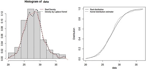
Female infertility and BMI: This study aims to investigate the body mass index (BMI) of infertile women of childbearing age. We use data from 200 participants from the Ben Badis University Hospital Centre of Constantine, Algeria, in 2018.

The first step is to establish the conformity test between the sample and a normal distribution. One obtain, D = 0.079226 smaller than p-value $\mathrm{0.1623.}$ This implies the use of the density and the distribution of the normal law. The second step is to estimate the density and the distribution functions and to represent them in a graph (Figure 1). For the MSE between the real density and a normal kernel density is equal to 0.003128583 and the rate of CSM convergence is 0.0008729775 and the AC convergence is $\mathrm{0.06541179.}$ We obtain for the distribution, MSE= 0.003128583 and the rate of CSM convergence is $0.0047592$ and the AC convergence is $\mathrm{0.1627624.}$ For the same rate of convergence, one have the MSE quantiles given by (25%, 0.0260281), (50%, 0.04186125), (75%,0.058767206). Note that the results of the real data come supported those of the simulation.

Figure 1. Density and distribution real data with density and distribution kernel estimate.

6. Conclusion

The present work proposed a new method to obtain the convergence rate of the MSE that is much more efficient in the CSMC case. Indeed, the CSM convergence rate gives better results than that of AC convergence. The previous results indicate that the choice of this type of convergence using kernel method estimate is a good alternative to the almost complete one. We can apply this type of convergence in any estimation that requires the study of the MSE, such as for example neural network, least squares method, …, and following the suggestion, it can be applied in neutrosophic statistics developed in Smarandache [27] and Afzal et al [28]. Moreover, maybe we can apply this type of convergence to extend the theorem of the law of large numbers.

Disclosure statement

No potential conflict of interest was reported by the authors.

Correction Statement

This article has been republished with minor changes. These changes do not impact the academic content of the article.

References

- Chow D. On the rate of moment convergence of sample function of a random variables with bounded support. Bull Inst Math Acd Sin. 1988;16:177–201.
- Liang H, Li D, Rosalsky A. Complete moment and integral convergence for sums of negatively associated random variables. Acta Math Sin (Engl Ser). 2010;26(3):419–432.
- Qui D, Chen P. Complete moment convergence for i.i.d random variables. Statist Probab Lett. 2014;91:76–82.
- Hsu P, Robbins H. Complete convergence and the law of large numbers. Proc Natl Acad Sci USA. 1947;33(2):25–31.
- Gut A, Stadtmüller U. An intermediate Baum–Katz theorem. Statist Probab Lett. 2011;81(10):1486–1492.
- Gut A. Marcinkiwicz laws and convergence rates in the law of large numbers for random variables with multidimensional indices. Ann Probab. 1978;6:469–482.
- Gut A. Convergence rates for probabilities of moderate deviations for sums of random variables with multidimensional indices. Ann Probab. 1980;8(2):298–313.
- Li D, Rao MB, Jiang T, et al. Complete convergence and almost sure convergence of weighted sums of random variables. J Theoret Probab. 1995;8(1):49–76.
- Sung SH. Complete convergence for weighted sums of random variables. Statist Probab Lett. 2007;77(3):303–311.
- Sung SH, Volodin A. On the rate of complete convergence for weighted sums of arrays of random elements. J Korean Math Soc. 2006;43(4):815–828.
- Rosenblatt M. Remarks on some non parametric estimates of a density function. Ann Math Statist. 1956;27(3):832–837.
- Parzen E. On estimation of a probability density function and mode. Ann Math Stat. 1962;33(3):1065–1076.
- Habbema JDF, Hermans J, Vanden Broee K. A stepwise discriminant analysis program using density estimation. In: Bruckmnann G, editor. Comp stat 1974, Proceedings in Computational Statistics. Vienna: Physica Verlag; 1974. p. 101–110.
- Hall P, Kang K-H. Bandwidth choice for non parametric classification. Ann Stat. 2005;33:284–306.
- Hall P, Wand MP. On non parametric discrimination using density differences. Biometrika. 1988;75(3):541–547.
- Ghosh AK, Chaudhuri P. Optimal smoothing in kernel analysis discriminant. Stat Sin. 2004;14:457–483.
- Ghosh AK, Hall P. On error-rate estimation in nonparametric classification. Stat Sin. 2008;18:1081–1100.
- Nadaraya EA. Some new estimates for distribution function. Theory of Probeb. Appl. 1964;9:497–500.
- Parzen E. Non parametric statistical data modelling. J Amer Stat Assoc. 1979;74(365):105–131.
- Baszczynska A. Kernel estimation of cumulative distribution function of a random variable with bounded support. Statist Trans. 2016;17:541–556.
- Azzalini A. A note on the estimation of a distribution function and quantiles by a kernel method. Biometrika. 1981;68(1):326–328.
- Sheather SJ, Marron JS. Kernel quantile estimators. J Amer Statist Assoc. 1990;85(410):410–416.
- Falk M. Relative deficiency of Kernel type estimators of quantiles. Ann Statist. 1984;12:261–268.
- David HA. Order statistics. 2nd ed. New York: John Wiley; 1981.
- Khan JA, Akbar A. Density estimation by Laplace kernel. Working paper. Department of Statistics, Bahauddin Zakariya, Multan, Pakistan. 2021.
- Chen SX. Probability density function estimation using gamma kernels. Ann Inst Statist Math. 2000;52(3):471–480.
- Smarandache F. Neutrosophic statistics vs. classical statistics, section in Nidus Idearum/superluminal physics. Vol. 7, 3rd ed. 2019. p. 117.
- Afzal U, Alrweili H, Ahamd N, et al. Neutrosophic statistical analysis of resistance depending on the temperature variance of conducting material. Sci Rep. 2021;11(1):Article ID 23939.
- Yu Y, et al. On the complete convergence for uncertain random variables. Soft Comput. 2022;26(3):1025–1031.