Numerical study of multi-order fractional differential equations with constant and variable coefficients

Abstract

In this manuscript, a numerical method based on the conjunction of Paraskevopoulos's algorithm and operational matrices is developed to solve numerically the multi-order linear and nonlinear fractional differential equations. By means of this conjunction, the multi-order problem is decomposed into a system of differential equations of fractional order which are then solved by employing operational matrices approach. The accuracy and efficiency of the method is examined by taking some examples. In addition, the numerical results presented in Pak et al. [Analytical solutions of linear inhomogeneous fractional differential equation with continuous variable coefficients. Adv Differ Equ. 2019;2019(256):1–22] are improved in our work.

Keywords:

• Multi-order fractional differential equations
• operational matrices
• shifted Legendre polynomials
• Caputo derivative
• Paraskevopoulos's method

2010 Mathematics Subject Classifications:

• 65M99
• 26A33
• 35R11
• 45K05

1. Introduction

Fractional calculus (FC) is a study of derivatives and integration of arbitrary order. At the initial phases of its development, it was considered as an abstract mathematical idea with nearly no applications. But, now the situation is entirely different with FC and it considered to be the most useful and important topic among the scientific community. The various important phenomena of science and engineering have been well described with the use of fractional derivatives, including, partial bed-load transport, diffusion model, dynamics of earthquakes, viscoelastic systems, biological systems, chaos, and wave propagation, (see [1–7]) and references therein. Furthermore, FDEs have been used in the modelling of important physical phenomena appearing in the study of control theory, electrostatic, study of polymers, visco-elasticity, signal and image processing phenomena, computer networking, and mathematical biology (see [8–13]) and references therein.

The exact solution of most of the fractional differential equations (FDEs) is difficult to find due to the involvement of the fractional differential and integral operators in the problem. So, it is a natural way to develop the numerical methods to solve them numerically. Operational matrices approach coupled with orthogonal polynomials is one of the efficient and stable numerical tool used to find the approximate solutions of fractional ordinary and partial differential equations (see [14–16]). This approach is easy in use which has the ability to transform the FDEs into a system of algebraic equations. Finally, this approach approximates the solution as basis vectors of orthogonal polynomials (see [17–21]).

Motivated by aforementioned studies, we propose a numerical method based on the extension of Paraskevopoulos's method in conjunction with shifted Legendre polynomials (SLPs) to solve numerically the multi-order linear and nonlinear FDEs with constant and variable coefficients. Under this approach, the multi-order fractional problem is decomposed into a system of FDEs which are then solved by using operational matrices approach. Finally, the solution is approximated as a basis vectors of orthogonal SLPs. We also compare the numerical results obtained using our method with the results obtained in [22]. We observe that our proposed method improves the numerical results presented in [22]. For instance, (see Example 7.5, Figure 1 and Table 1).

Figure 1. The maximum absolute errors determined by our method are compared with the maximum absolute errors determined by the method ([22], Example 2, n = 3. (a) (Our proposed method) and (b) (Proposed method in [22])).

Table 1. Maximum absolute error of Example 7.5 at $n=\{2,3,4,6\}$=scale level=number of terms of SLPs, and for different values of t.

t	n = 2	n = 3	n = 4	n = 6
0.0	0.0000	0.0000	0.0000	$4.5537\times {10}^{-41}$
0.2	$2.3616\times {10}^{-3}$	$6.7672\times {10}^{-4}$	$1.1310\times {10}^{-4}$	$5.4764\times {10}^{-5}$
0.4	$3.2289\times {10}^{-3}$	$1.7558\times {10}^{-4}$	$2.3608\times {10}^{-4}$	$5.0444\times {10}^{-5}$
0.6	$2.6020\times {10}^{-3}$	$5.7017\times {10}^{-4}$	$1.0341\times {10}^{-4}$	$7.8996\times {10}^{-6}$
0.8	$4.8096\times {10}^{-4}$	$6.2728\times {10}^{-4}$	$3.2997\times {10}^{-4}$	$4.8405\times {10}^{-5}$
1.0	$3.1343\times {10}^{-3}$	$9.3751\times {10}^{-4}$	$2.4238\times {10}^{-4}$	$4.7670\times {10}^{-5}$

The manuscript is organized as follows: Some essential definitions, properties and results of FC are given in Section 2. In Section 3, the properties of SLPs are recalled. In Section 4, a generalized operational matrix in the sense of Caputo fractional differential operator is studied. In Section 5, the multi-order fractional problems are reduced into a system of FDEs. In Section 6, a numerical algorithm based on Paraskevopoulos's method in conjunction with operational matrices approach is developed to solve linear and nonlinear multi-order FDEs with constant and variable coefficients. The numerical accuracy of the proposed method is examined by taking some examples in Section 7. Finally, in Section 9, the manuscript ends with a brief conclusion and some remarks.

2. Preliminary remarks on FC

Some important definitions and results are recalled in this section which are indispensable to construct the proposed numerical algorithm.

Definition 2.1

The (left side) Riemann–Liouville integral of order $\alpha >0$ is given as (see [10]): (1) $J^{\alpha }u(t)=\frac{1}{\mathrm{\Gamma }(\alpha )}{\int }_0^t(t-s{)}^{\alpha -1}u(s)\mathrm{d}s,t>0.$(1)

Definition 2.2

The (left side) Riemann-Liouville derivative of order $\alpha >0$ is given as (see [10]): (2) ${}_{RL}{\mathcal{D}}^{\alpha }u(t)=D^m{J}^{m-\alpha }u(t),m-1<\alpha \le m,m\in \mathbb{N}.$(2)

Definition 2.3

The (left side) Caputo derivative of order $\alpha >0$ is given as (see [10]): (3) ${}_C{\mathcal{D}}^{\alpha }u(t)=\{\begin{array}{lll}{\displaystyle \frac{{\mathrm{d}}^{m}u(t)}{\mathrm{d}{t}^m}},& \alpha =m\in \mathbb{N},J^{m-\alpha }{u}^{(m)}(t),& m-1<\alpha <m,m\in \mathbb{N},\end{array}$(3) where m is an integer, t>0, and $u(t)\in C^m[0,1]$.

For the Caputo derivative, we have the following observations: (4) $\begin{array}{rl}{}_C{\mathcal{D}}^{\alpha }K& =0,K\mathrm{is}\mathrm{a}\mathrm{constant}.\end{array}$(4) (5) $\begin{array}{rl}{}_C{\mathcal{D}}^{\alpha }{t}^{\mu }& =\{\begin{array}{lll}0,& \mathrm{for}\mu \in {\mathbb{R}}_{\mathbb{+}},\text{and}\mu <\lceil \alpha \rceil ,{\displaystyle \frac{\mathrm{\Gamma }(\mu +1)}{\mathrm{\Gamma }(\mu +1-\alpha )}}{t}^{\mu -\alpha },& \begin{array}{l}\mathrm{for}\mu \in {\mathbb{R}}_{\mathbb{+}},\text{and}\mu \ge \lceil \alpha \rceil .\end{array}\end{array}\end{array}$(5) Note the following basic results: ${}_{RL}{\mathcal{D}}^{\gamma }{J}^{\alpha }u(t)=\{\begin{array}{ll}{J}^{\alpha -\gamma }u(t),& \mathrm{if}\alpha >\gamma .\\ u(t),& \mathrm{if}\alpha =\gamma .\\ J^{\gamma -\alpha }u(t),& \mathrm{if}\alpha <\gamma .\end{array}$

Lemma 2.1

Let $u(t)\in C^n[0,1]$ for $n\in \mathbb{N}$, and suppose $n\ge m$, $\alpha \in {\mathbb{R}}_{\mathbb{+}}\setminus \mathbb{N}$, such that, $0<\alpha <n$. Then, ${}_C{\mathcal{D}}^{\alpha }u(0)=0$.

Proof.

By definition of Caputo differential operator, we have (6) $\begin{array}{rl}{}_C{\mathcal{D}}^{\alpha }u(t)& =J^{m-\alpha }{u}^{(m)}(t)\\ & =\frac{1}{\mathrm{\Gamma }(m-\alpha )}{\int }_0^t\frac{u^{(m)}(t)}{(t-s{)}^{1-m+\alpha }}\mathrm{d}s,\end{array}$(6) where m is an integer defined as $m-1<\alpha <m$. Now, according to our assumption, $n\ge m$ which implies that $u^{(m)}(t)$ is a continuous function, and $u^{(m)}(t)\in C^{n-m}[0,1]$. Consequently, for $t\to 0$, the integral in (6(6) $\begin{array}{rl}{}_C{\mathcal{D}}^{\alpha }u(t)& =J^{m-\alpha }{u}^{(m)}(t)\\ & =\frac{1}{\mathrm{\Gamma }(m-\alpha )}{\int }_0^t\frac{u^{(m)}(t)}{(t-s{)}^{1-m+\alpha }}\mathrm{d}s,\end{array}$(6) ) vanishes. Hence, ${}_C{\mathcal{D}}^{\alpha }u(0)=0$.

3. Properties of SLPs

The following recurrence formulae are used to evaluate the orthogonal Legendre polynomials (LPs) on the interval of orthogonality $[-1,1]$ (see [23]): (7) $\begin{array}{rl}& P_{j+1}(x)=\frac{2j+1}{j+1}x{P}_j(x)-\frac{j}{j+1}{P}_{j-1}(x),j=1,2,\dots ,\\ & \mathrm{where}\\ & P_0(x)=1,P_1(x)=x.\end{array}$(7) Now by setting, x = 2t−1 in (7(7) $\begin{array}{rl}& P_{j+1}(x)=\frac{2j+1}{j+1}x{P}_j(x)-\frac{j}{j+1}{P}_{j-1}(x),j=1,2,\dots ,\\ & \mathrm{where}\\ & P_0(x)=1,P_1(x)=x.\end{array}$(7) ), the SLPs on the interval of orthogonality $[0,1]$ can be expressed with the aid of the following analytical form, (see [23]) (8) $\widetilde{P_j}(t)=\sum _{k=0}^j(-1{)}^{k+j}\frac{(k+j)!}{(j-k)!(k!{)}^2}{t}^k.$(8) The orthogonality condition of SLPs can be expressed as (9) ${\int }_0^1\widetilde{P_j}(t)\widetilde{P_i}(t)\mathrm{d}t=\{\begin{array}{lll}{\displaystyle \frac{1}{2j+1}},& \mathrm{for}j=i,0,& \mathrm{for}j\ne i.\end{array}$(9)

3.1. Functions approximation

Suppose $u(t)\in L^2[0,1]$, then it can be demonstrated as a basis vectors of SLPs, (see [23]) (10) $u(t)=\sum _{i=0}^{\mathrm{\infty }}{e}_i\widetilde{P_i}(t).$(10) Using (9(9) ${\int }_0^1\widetilde{P_j}(t)\widetilde{P_i}(t)\mathrm{d}t=\{\begin{array}{lll}{\displaystyle \frac{1}{2j+1}},& \mathrm{for}j=i,0,& \mathrm{for}j\ne i.\end{array}$(9) ), the coefficients $e_i$ can be determined as (11) $e_i=(2i+1){\int }_0^{1}u(t)\widetilde{P_i}(t)\mathrm{d}t,i=0,1,2,\dots .$(11) For the practicality, considering the first n + 1-terms of (10(10) $u(t)=\sum _{i=0}^{\mathrm{\infty }}{e}_i\widetilde{P_i}(t).$(10) ), we have (12) $\begin{array}{rl}u(t)& \simeq \sum _{i=0}^n{e}_i\widetilde{P_i}(t),\\ & =(\mathrm{\Lambda }{)}^T\mathrm{\Psi }(t),\end{array}$(12) where (13) $(\mathrm{\Lambda }{)}^T=[e_0,e_1,\dots ,e_n],$(13) and (14) $\mathrm{\Psi }(t)=\left[\begin{array}{c}\widetilde{P_0}(t)\\ \widetilde{P_1}(t)\\ ⋮\\ \widetilde{P_n}(t)\end{array}\right].$(14)

4. Generalized derivative operational matrix of SLPs in Caputo sense

Lemma 4.1

Let $\mathrm{\Psi }(t)$ be defined in (14(14) $\mathrm{\Psi }(t)=\left[\begin{array}{c}\widetilde{P_0}(t)\\ \widetilde{P_1}(t)\\ ⋮\\ \widetilde{P_n}(t)\end{array}\right].$(14) ), then $($see [24]$)$ (15) $\frac{\mathrm{d}\mathrm{\Psi }(t)}{\mathrm{d}t}={\mathbf{D}}^{(1)}\mathrm{\Psi }(t),$(15) where (16) $\begin{array}{rl}{\mathbf{D}}^{(1)}& =d_{(p+1,q+1)}\\ & =\{\begin{array}{l}2(2q+1),q=p-r\\ \{\begin{array}{l}r=1,3,\dots m,p=1,2,\dots ,m,\text{if m odd;}\\ r=1,3,\dots m-1,p=1,2,\dots ,m,\text{if m even.}\end{array}\\ 0,\mathrm{otherwise}.\end{array}\end{array}$(16) For example, for m = 9, we have $\begin{array}{rl}{\mathbf{D}}^{(1)}& =(\begin{array}{cccc}0& 0& 0& 0\\ 2.0000& 0& 0& 0\\ 0& 6.0000& 0& 0\\ 2.0000& 0& 10.0000& 0\\ 0& 6.0000& 0& 14.0000\\ 2.0000& 0& 10.0000& 0\\ 0& 6.0000& 0& 14.0000\\ 2.0000& 0& 10.0000& 0\\ 0& 6.0000& 0& 14.0000\\ 2.0000& 0& 10.0000& 0\end{array}\\ & \begin{array}{cccc}0& 0& 0& 0\\ 0& 0& 0& 0\\ 0& 0& 0& 0\\ 0& 0& 0& 0\\ 0& 0& 0& 0\\ 18.0000& 0& 0& 0\\ 0& 22.0000& 0& 0\\ 18.0000& 0& 26.0000& 0\\ 0& 22.0000& 0& 30.0000\\ 18.0000& 0& 26.0000& 0.0000\end{array}\\ & \begin{array}{cc}0& 0\\ 0& 0\\ 0& 0\\ 0& 0\\ 0& 0\\ 0& 0\\ 0& 0\\ 0& 0\\ 0& 0.0000\\ 34.0000& 0\end{array})\end{array}$

In general for m odd, we have $\begin{array}{rl}{\mathbf{D}}^{(1)}& =(\begin{array}{cccccc}0& 0& 0& 0& 0& \cdots \\ 2& 0& 0& 0& 0& \cdots \\ 0& 6& 0& 0& 0& \cdots \\ 2& 0& 10& 0& 0& \cdots \\ 0& 6& 0& 14& 0& \cdots \\ ⋮& ⋮& ⋮& ⋮& ⋮& ⋮\\ 0& 6& 0& 14& 0& \cdots \\ 2& 0& 10& 0& 18& \cdots \end{array}\\ & \begin{array}{ccc}0& 0& 0\\ 0& 0& 0\\ 0& 0& 0\\ 0& 0& 0\\ 0& 0& 0\\ ⋮& ⋮& ⋮\\ 2(2n-3)& 0& 0\\ 0& 2(2n-1)& 0\end{array}),\end{array}$and for m even, we have $\begin{array}{rl}{\mathbf{D}}^{(1)}& =(\begin{array}{cccccc}0& 0& 0& 0& 0& \cdots \\ 2& 0& 0& 0& 0& \cdots \\ 0& 6& 0& 0& 0& \cdots \\ 2& 0& 10& 0& 0& \cdots \\ 0& 6& 0& 14& 0& \cdots \\ ⋮& ⋮& ⋮& ⋮& ⋮& ⋮\\ 2& 0& 10& 0& 18& \cdots \\ 0& 6& 0& 14& 0& \cdots \end{array}\\ & \begin{array}{ccc}0& 0& 0\\ 0& 0& 0\\ 0& 0& 0\\ 0& 0& 0\\ 0& 0& 0\\ ⋮& ⋮& ⋮\\ 2(2n-3)& 0& 0\\ 0& 2(2n-1)& 0\end{array}).\end{array}$

Lemma 4.2

Let $\widetilde{P_j}(t)$ be the SLPs as defined in (8(8) $\widetilde{P_j}(t)=\sum _{k=0}^j(-1{)}^{k+j}\frac{(k+j)!}{(j-k)!(k!{)}^2}{t}^k.$(8) ), then ${}_C{\mathcal{D}}^{\alpha }\widetilde{P_j}(t)=0,j=0,1,\dots ,\lceil \alpha \rceil -1,\alpha >0$.

Proof.

Using the definition of SLPs, we have (17) $\begin{array}{rl}\widetilde{P_j}(t)& =\sum _{k=0}^j(-1{)}^{k+j}\frac{(k+j)!}{(j-k)!(k!{)}^2}{t}^k,\\ & j=0,1,\dots ,\lceil \alpha \rceil -1.\end{array}$(17) Using (17(17) $\begin{array}{rl}\widetilde{P_j}(t)& =\sum _{k=0}^j(-1{)}^{k+j}\frac{(k+j)!}{(j-k)!(k!{)}^2}{t}^k,\\ & j=0,1,\dots ,\lceil \alpha \rceil -1.\end{array}$(17) ), the SLPs of degree $\lceil \alpha \rceil -1$ is demonstrated as (18) $\begin{array}{rl}\widetilde{P_{\lceil \alpha \rceil -1}}(t)& =\frac{(-1{)}^{\lceil \alpha \rceil -1}(\lceil \alpha \rceil -1)!}{(\lceil \alpha \rceil -1)!}{t}^0\\ & +\frac{(-1{)}^{\lceil \alpha \rceil }(\lceil \alpha \rceil )!}{(\lceil \alpha \rceil -2)!}{t}^1\\ & +\frac{(-1{)}^{\lceil \alpha \rceil +1}(\lceil \alpha \rceil +1)!}{4(\lceil \alpha \rceil -3)!}{t}^2+\cdots \\ & +\frac{(-1{)}^{2(\lceil \alpha \rceil -1)}(2(\lceil \alpha \rceil -1))!}{(\lceil 2\alpha \rceil )!(\lceil \alpha \rceil -1)!{)}^2}{t}^{\lceil \alpha \rceil -1}.\end{array}$(18) Applying Caputo differential operator, and its linearity to (18(18) $\begin{array}{rl}\widetilde{P_{\lceil \alpha \rceil -1}}(t)& =\frac{(-1{)}^{\lceil \alpha \rceil -1}(\lceil \alpha \rceil -1)!}{(\lceil \alpha \rceil -1)!}{t}^0\\ & +\frac{(-1{)}^{\lceil \alpha \rceil }(\lceil \alpha \rceil )!}{(\lceil \alpha \rceil -2)!}{t}^1\\ & +\frac{(-1{)}^{\lceil \alpha \rceil +1}(\lceil \alpha \rceil +1)!}{4(\lceil \alpha \rceil -3)!}{t}^2+\cdots \\ & +\frac{(-1{)}^{2(\lceil \alpha \rceil -1)}(2(\lceil \alpha \rceil -1))!}{(\lceil 2\alpha \rceil )!(\lceil \alpha \rceil -1)!{)}^2}{t}^{\lceil \alpha \rceil -1}.\end{array}$(18) ), we have (19) $\begin{array}{rl}{}_C{\mathcal{D}}^{\alpha }\widetilde{P_{\lceil \alpha \rceil -1}}(t)& ={\frac{(-1{)}^{\lceil \alpha \rceil -1}(\lceil \alpha \rceil -1)!}{(\lceil \alpha \rceil -1)!}}_C{\mathcal{D}}^{\alpha }{t}^0\\ & +{\frac{(-1{)}^{\lceil \alpha \rceil }(\lceil \alpha \rceil )!}{(\lceil \alpha \rceil -2)!}}_C{\mathcal{D}}^{\alpha }{t}^1\\ & +{\frac{(-1{)}^{\lceil \alpha \rceil +1}(\lceil \alpha \rceil +1)!}{4(\lceil \alpha \rceil -3)!}}_C{\mathcal{D}}^{\alpha }{t}^2+\cdots \\ & +{\frac{(-1{)}^{2(\lceil \alpha \rceil -1)}(2(\lceil \alpha \rceil -1))!}{(\lceil 2\alpha \rceil )!(\lceil \alpha \rceil -1)!{)}^2}}_C{\mathcal{D}}^{\alpha }{t}^{\lceil \alpha \rceil -1}.\end{array}$(19) Since, $\alpha >\lceil \alpha \rceil -1$, then using the results of (4(4) $\begin{array}{rl}{}_C{\mathcal{D}}^{\alpha }K& =0,K\mathrm{is}\mathrm{a}\mathrm{constant}.\end{array}$(4) )–(5(5) $\begin{array}{rl}{}_C{\mathcal{D}}^{\alpha }{t}^{\mu }& =\{\begin{array}{lll}0,& \mathrm{for}\mu \in {\mathbb{R}}_{\mathbb{+}},\text{and}\mu <\lceil \alpha \rceil ,{\displaystyle \frac{\mathrm{\Gamma }(\mu +1)}{\mathrm{\Gamma }(\mu +1-\alpha )}}{t}^{\mu -\alpha },& \begin{array}{l}\mathrm{for}\mu \in {\mathbb{R}}_{\mathbb{+}},\text{and}\mu \ge \lceil \alpha \rceil .\end{array}\end{array}\end{array}$(5) ), we have (20) ${}_C{\mathcal{D}}^{\alpha }\widetilde{P_{\lceil \alpha \rceil -1}}(t)=0.$(20) Consequently, (21) ${}_C{\mathcal{D}}^{\alpha }\widetilde{P_j}(t)=0,j=0,1,\dots ,\lceil \alpha \rceil -1,\alpha >0.$(21)

Theorem 4.1

Let $\mathrm{\Psi }(t)$ be a function vector of SLPs and suppose $\alpha >0$, then (22) ${}_C{\mathcal{D}}^{\alpha }\mathrm{\Psi }(t)\simeq {\mathbf{D}}^{(\alpha )}\mathrm{\Psi }(t)$(22) where ${\mathbf{D}}^{(\alpha )}$ is a generalized derivative operational matrix in Caputo sense, demonstrated as (23) $\begin{array}{rl}{\mathbf{D}}^{(\alpha )}& =(\begin{array}{ccc}0& 0& 0\\ ⋮& ⋮& ⋮\\ 0& 0& 0\\ {\mathrm{\Omega }}_{\alpha }(\lceil \alpha \rceil ,0)& {\mathrm{\Omega }}_{\alpha }(\lceil \alpha \rceil ,1)& {\mathrm{\Omega }}_{\alpha }(\lceil \alpha \rceil ,2)\\ ⋮& ⋮& ⋮\\ {\mathrm{\Omega }}_{\alpha }(j,0)& {\mathrm{\Omega }}_{\alpha }(j,1)& {\mathrm{\Omega }}_{\alpha }(j,2)\\ ⋮& ⋮& ⋮\\ {\mathrm{\Omega }}_{\alpha }(n,0)& {\mathrm{\Omega }}_{\alpha }(n,1)& {\mathrm{\Omega }}_{\alpha }(n,2)\end{array}\\ & \begin{array}{cc}\cdots & 1\\ \cdots & ⋮\\ \cdots & 0\\ \cdots & {\mathrm{\Omega }}_{\alpha }(\lceil \alpha \rceil ,m)\\ \cdots & ⋮\\ \cdots & {\mathrm{\Omega }}_{\alpha }(j,n)\\ \cdots & ⋮\\ \cdots & {\mathrm{\Omega }}_{\alpha }(n,n)\end{array})\end{array}$(23) where $\begin{array}{rl}{\mathrm{\Omega }}_{\alpha }(j,l)& =\sum _{k=\lceil \alpha \rceil }^j{\mathrm{{\rm Y}}}_{j,l,k},\end{array}$and ${\mathrm{{\rm Y}}}_{j,l,k}$ is given as (24) $\begin{array}{rl}{\mathrm{{\rm Y}}}_{j,l,k}& =(2l+1)\sum _{r=0}^l\frac{\begin{array}{c}(-1{)}^{j+k+l+r}\\ \mathrm{\Gamma }(j+k+1)\mathrm{\Gamma }(l+r+1)\end{array}}{\begin{array}{c}\mathrm{\Gamma }(j-k+1)\mathrm{\Gamma }(k+1)\\ \mathrm{\Gamma }(k+1-\alpha )\mathrm{\Gamma }(l-r+1)\\ (\mathrm{\Gamma }(r+1){)}^2\end{array}}\\ & \times \frac{1}{(k+r-\alpha +1)},l=0,1,\dots ,n.\end{array}$(24)

Proof.

Using (8(8) $\widetilde{P_j}(t)=\sum _{k=0}^j(-1{)}^{k+j}\frac{(k+j)!}{(j-k)!(k!{)}^2}{t}^k.$(8) ), (5(5) $\begin{array}{rl}{}_C{\mathcal{D}}^{\alpha }{t}^{\mu }& =\{\begin{array}{lll}0,& \mathrm{for}\mu \in {\mathbb{R}}_{\mathbb{+}},\text{and}\mu <\lceil \alpha \rceil ,{\displaystyle \frac{\mathrm{\Gamma }(\mu +1)}{\mathrm{\Gamma }(\mu +1-\alpha )}}{t}^{\mu -\alpha },& \begin{array}{l}\mathrm{for}\mu \in {\mathbb{R}}_{\mathbb{+}},\text{and}\mu \ge \lceil \alpha \rceil .\end{array}\end{array}\end{array}$(5) ), and Lemma 4.2, we have (25) $\begin{array}{rl}{}_C{\mathcal{D}}^{\alpha }\widetilde{P_j}(t)& =\sum _{k=\lceil \alpha \rceil }^j(-1{)}^{k+j}\frac{\mathrm{\Gamma }(1+k+j)}{\begin{array}{c}\mathrm{\Gamma }(1-k+j)\mathrm{\Gamma }(1+k)\\ \mathrm{\Gamma }(1+k-\alpha )\end{array}}{t}^{k-\alpha }.\end{array}$(25) We can approximate $t^{k-\alpha }$ by first n + 1-terms of SLPs, as (26) $t^{k-\alpha }\simeq \sum _{l=0}^n{e}_{l,k}\widetilde{P_l}(t),$(26) where (27) $\begin{array}{rl}{e}_{l,k}& =(2l+1){\int }_0^1{t}^{k-\alpha }\widetilde{P_l}(t)\mathrm{d}t\\ & =(2l+1)\sum _{r=0}^l\frac{(-1{)}^{l+r}\mathrm{\Gamma }(l+r+1)}{\mathrm{\Gamma }(l-r+1)(\mathrm{\Gamma }(r+1){)}^2}\\ & \times {\int }_0^1{t}^{k+r-\alpha }\mathrm{d}t\\ & =(2l+1)\sum _{r=0}^l\frac{(-1{)}^{l+r}\mathrm{\Gamma }(l+r+1)}{\begin{array}{c}\mathrm{\Gamma }(l-r+1)(\mathrm{\Gamma }(r+1){)}^2\\ (k+r-\alpha +1)\end{array}}\end{array}$(27) By inserting, (26(26) $t^{k-\alpha }\simeq \sum _{l=0}^n{e}_{l,k}\widetilde{P_l}(t),$(26) ) into (25(25) $\begin{array}{rl}{}_C{\mathcal{D}}^{\alpha }\widetilde{P_j}(t)& =\sum _{k=\lceil \alpha \rceil }^j(-1{)}^{k+j}\frac{\mathrm{\Gamma }(1+k+j)}{\begin{array}{c}\mathrm{\Gamma }(1-k+j)\mathrm{\Gamma }(1+k)\\ \mathrm{\Gamma }(1+k-\alpha )\end{array}}{t}^{k-\alpha }.\end{array}$(25) ), we have (28) ${}_C{\mathcal{D}}^{\alpha }\widetilde{P_j}(t)\simeq \sum _{k=\lceil \alpha \rceil }^j\sum _{l=0}^n\frac{(-1{)}^{j+k}\mathrm{\Gamma }(j+k+1)}{\begin{array}{c}\mathrm{\Gamma }(j-k+1)\mathrm{\Gamma }(k+1)\\ \mathrm{\Gamma }(k+1-\alpha )\end{array}}{e}_{l,k}\widetilde{P_l}(t).$(28) By putting the value of $e_{l,k}$ in (28(28) ${}_C{\mathcal{D}}^{\alpha }\widetilde{P_j}(t)\simeq \sum _{k=\lceil \alpha \rceil }^j\sum _{l=0}^n\frac{(-1{)}^{j+k}\mathrm{\Gamma }(j+k+1)}{\begin{array}{c}\mathrm{\Gamma }(j-k+1)\mathrm{\Gamma }(k+1)\\ \mathrm{\Gamma }(k+1-\alpha )\end{array}}{e}_{l,k}\widetilde{P_l}(t).$(28) ), and after some simplification, we have (29) $\begin{array}{rl}{}_C{\mathcal{D}}^{\alpha }\widetilde{P_j}(t)& \simeq \sum _{k=\lceil \alpha \rceil }^j\sum _{l=0}^n(2l+1)\\ & \times \sum _{r=0}^l\frac{\begin{array}{c}(-1{)}^{j+k+l+r}\mathrm{\Gamma }(j+k+1)\\ \mathrm{\Gamma }(l+r+1)\end{array}}{\begin{array}{c}\mathrm{\Gamma }(j-k+1)\mathrm{\Gamma }(k+1)\mathrm{\Gamma }(k+1-\alpha )\\ \mathrm{\Gamma }(l-r+1)(\mathrm{\Gamma }(r+1){)}^2\end{array}}\\ & \times \frac{1}{(k+r-\alpha +1)}\widetilde{P_l}(t).\end{array}$(29) For simplicity, we have (30) $\begin{array}{rl}{\mathrm{{\rm Y}}}_{j,l,k}& =(2l+1)\sum _{r=0}^l\frac{\begin{array}{c}(-1{)}^{j+k+l+r}\mathrm{\Gamma }(j+k+1)\\ \mathrm{\Gamma }(l+r+1)\end{array}}{\begin{array}{c}\mathrm{\Gamma }(j-k+1)\mathrm{\Gamma }(k+1)\mathrm{\Gamma }(k+1-\alpha )\\ \mathrm{\Gamma }(l-r+1)(\mathrm{\Gamma }(r+1){)}^2\end{array}}\\ & \times \frac{1}{(k+r-\alpha +1)}.\end{array}$(30) Now (29(29) $\begin{array}{rl}{}_C{\mathcal{D}}^{\alpha }\widetilde{P_j}(t)& \simeq \sum _{k=\lceil \alpha \rceil }^j\sum _{l=0}^n(2l+1)\\ & \times \sum _{r=0}^l\frac{\begin{array}{c}(-1{)}^{j+k+l+r}\mathrm{\Gamma }(j+k+1)\\ \mathrm{\Gamma }(l+r+1)\end{array}}{\begin{array}{c}\mathrm{\Gamma }(j-k+1)\mathrm{\Gamma }(k+1)\mathrm{\Gamma }(k+1-\alpha )\\ \mathrm{\Gamma }(l-r+1)(\mathrm{\Gamma }(r+1){)}^2\end{array}}\\ & \times \frac{1}{(k+r-\alpha +1)}\widetilde{P_l}(t).\end{array}$(29) ) can be expressed as (31) ${}_C{\mathcal{D}}^{\alpha }\widetilde{P_j}(t)\simeq \sum _{k=\lceil \alpha \rceil }^j\sum _{l=0}^n{\mathrm{{\rm Y}}}_{j,l,k}\widetilde{P_l}(t),j=\lceil \alpha \rceil ,\dots ,m.$(31) (31(31) ${}_C{\mathcal{D}}^{\alpha }\widetilde{P_j}(t)\simeq \sum _{k=\lceil \alpha \rceil }^j\sum _{l=0}^n{\mathrm{{\rm Y}}}_{j,l,k}\widetilde{P_l}(t),j=\lceil \alpha \rceil ,\dots ,m.$(31) ) can be written in vector notation as (32) $\begin{array}{rl}& {}_C{\mathcal{D}}^{\alpha }\widetilde{P_j}(t)\\ & \simeq [\sum _{k=\lceil \alpha \rceil }^j{\mathrm{{\rm Y}}}_{j,0,k},\sum _{k=\lceil \alpha \rceil }^j{\mathrm{{\rm Y}}}_{j,1,k},\dots ,\sum _{k=\lceil \alpha \rceil }^j{\mathrm{{\rm Y}}}_{j,n,k}]\mathrm{\Psi }(t),\\ & j=\lceil \alpha \rceil ,\dots ,n.\end{array}$(32) Moreover, using Lemma 4.2, we have (33) ${}_C{\mathcal{D}}^{\alpha }\widetilde{P_j}(t)=[0,0,\dots ,0]\mathrm{\Psi }(t),j=0,1,\dots ,\lceil \alpha \rceil -1.$(33) Equations (32(32) $\begin{array}{rl}& {}_C{\mathcal{D}}^{\alpha }\widetilde{P_j}(t)\\ & \simeq [\sum _{k=\lceil \alpha \rceil }^j{\mathrm{{\rm Y}}}_{j,0,k},\sum _{k=\lceil \alpha \rceil }^j{\mathrm{{\rm Y}}}_{j,1,k},\dots ,\sum _{k=\lceil \alpha \rceil }^j{\mathrm{{\rm Y}}}_{j,n,k}]\mathrm{\Psi }(t),\\ & j=\lceil \alpha \rceil ,\dots ,n.\end{array}$(32) ) and (33(33) ${}_C{\mathcal{D}}^{\alpha }\widetilde{P_j}(t)=[0,0,\dots ,0]\mathrm{\Psi }(t),j=0,1,\dots ,\lceil \alpha \rceil -1.$(33) ) together prove the required result.

5. Decomposition of multi-order FDEs into a system of FDEs

Consider the multi-order FDEs as (34) $\begin{array}{rl}{}_C{\mathcal{D}}^{\alpha }u(t)& =f(t,u(t){,}_C{\mathcal{D}}^{{\beta }_1}u(t){,}_C{\mathcal{D}}^{{\beta }_2}u(t),\dots ,{}_C{\mathcal{D}}^{{\beta }_n}u(t)),\\ & u^{(k)}(0)=d_k,k=0,1,\dots ,m.\end{array}$(34) where $m-1<\alpha \le m$, $0<{\beta }_1<{\beta }_2<\cdots <{\beta }_n<\alpha$, f can be a nonlinear in general, and ${}_C{\mathcal{D}}^{\alpha }$ is a Caputo derivative of order α defined in (3(3) ${}_C{\mathcal{D}}^{\alpha }u(t)=\{\begin{array}{lll}{\displaystyle \frac{{\mathrm{d}}^{m}u(t)}{\mathrm{d}{t}^m}},& \alpha =m\in \mathbb{N},J^{m-\alpha }{u}^{(m)}(t),& m-1<\alpha <m,m\in \mathbb{N},\end{array}$(3) ). Problem (34(34) $\begin{array}{rl}{}_C{\mathcal{D}}^{\alpha }u(t)& =f(t,u(t){,}_C{\mathcal{D}}^{{\beta }_1}u(t){,}_C{\mathcal{D}}^{{\beta }_2}u(t),\dots ,{}_C{\mathcal{D}}^{{\beta }_n}u(t)),\\ & u^{(k)}(0)=d_k,k=0,1,\dots ,m.\end{array}$(34) ) can be decomposed into a system of FDEs, as

Set $u_1=u$ and suppose, (35) ${}_C{\mathcal{D}}^{{\beta }_1}{u}_1=u_2.$(35) Case(1) If $m-1\le {\beta }_1<{\beta }_2\le m$, then we define (36) ${}_C{\mathcal{D}}^{{\beta }_2-{\beta }_1}{u}_2=u_3.$(36) Claim: $u_3={}_C{\mathcal{D}}^{{\beta }_2}u$.

If ${\beta }_1=m-1$, then ${}_C{\mathcal{D}}^{{\beta }_2-\beta 1}{u}_2={}_C{\mathcal{D}}^{{\beta }_2-(m-1)}{.}_C{\mathcal{D}}^{(m-1)}{u}_1={}_C{\mathcal{D}}^{{\beta }_2}{u}_1={}_C{\mathcal{D}}^{{\beta }_2}u$.

Hence the claim is verified.

If ${\beta }_1\notin \mathbb{N}$, then by Lemma 2.1, ${}_C{\mathcal{D}}^{{\beta }_1}{u}_1(0)=0$, and as ${\beta }_2-{\beta }_1<1$, $\begin{array}{rl}{}_C{\mathcal{D}}^{{\beta }_2-{\beta }_1}{[}_C{\mathcal{D}}^{{\beta }_1}{u}_1]& {=}_{RL}{\mathcal{D}}^{{\beta }_2-{\beta }_1}{[}_C{\mathcal{D}}^{{\beta }_1}{u}_1]\\ & =D{J}^{1+{\beta }_1-{\beta }_2}{J}^{m-{\beta }_1}{u}_1^{(m)}\\ & =D{J}^{1+m-{\beta }_2}{u}_1^{(m)}=J^{m-{\beta }_2}{u}_1^{(m)}\\ & ={}_C{\mathcal{D}}^{{\beta }_2}{u}_1={}_C{\mathcal{D}}^{{\beta }_2}u.\end{array}$Therefore $u_3={}_C{\mathcal{D}}^{{\beta }_2-{\beta }_1}{u}_2={}_C{\mathcal{D}}^{{\beta }_2}u$.

Case (2) Consider $m-1\le {\beta }_1<m\le {\beta }_2$. If ${\beta }_1=m-1$, then define (37) ${}_C{\mathcal{D}}^{{\beta }_2-\beta 1}{u}_2=u_3.$(37) As ${}_C{\mathcal{D}}^{{\beta }_2-{\beta }_1}{u}_2={}_C{\mathcal{D}}^{{\beta }_2-m+1}{.}_C{\mathcal{D}}^{m-1}{u}_1={}_C{\mathcal{D}}^{{\beta }_2}{u}_1$.

If $m-1<{\beta }_1<m\le {\beta }_2$, then define, (38) ${}_C{\mathcal{D}}^{m-{\beta }_1}{u}_2=u_3.$(38) Claim: $u_3=u^{(m)}$. As ${\beta }_1\notin \mathbb{N}$, then by Lemma 2.1$,{}_C{\mathcal{D}}^{{\beta }_1}{u}_1(0)=u_2(0)=0$ and $0<m-{\beta }_1<1$, ${}_C{\mathcal{D}}^{m-{\beta }_1}{u}_2{=}_{RL}{\mathcal{D}}^{m-{\beta }_1}{.}_C{\mathcal{D}}^{{\beta }_1}{u}_1=D{J}^{1+{\beta }_1-m}{J}^{m-{\beta }_1}{u}_1^{(m)}=DJ{u}_1^{(m)}=u_1^{(m)}=u^{(m)}$.

Hence $u_3=u^{(m)}$. Further, we define: (39) ${}_C{\mathcal{D}}^{{\beta }_2-m}{u}_3=u_4.$(39) Claim: $u_4={}_C{\mathcal{D}}^{{\beta }_2}u.$ As $u_4={}_C{\mathcal{D}}^{{\beta }_2-m}{u}_3{=}_C{\mathcal{D}}^{{\beta }_2-m}{u}^{(m)}={}_C{\mathcal{D}}^{{\beta }_2}u$.

The process will be continued until the decomposition of the problem (34(34) $\begin{array}{rl}{}_C{\mathcal{D}}^{\alpha }u(t)& =f(t,u(t){,}_C{\mathcal{D}}^{{\beta }_1}u(t){,}_C{\mathcal{D}}^{{\beta }_2}u(t),\dots ,{}_C{\mathcal{D}}^{{\beta }_n}u(t)),\\ & u^{(k)}(0)=d_k,k=0,1,\dots ,m.\end{array}$(34) ) into a system of FDEs.

5.1. Implementation to the problem

In this section, a multi-order fractional differential equation is decomposed into a system of FDEs using the algorithm developed in Section 5.

Consider the following multi-order fractional differential equation (40) $\begin{array}{rl}& u^{\mathrm{\prime }\mathrm{\prime }\mathrm{\prime }}(t){+}_C{\mathcal{D}}^{\frac{5}{2}}u(t)+u^{\mathrm{\prime }\mathrm{\prime }}(t)+4u^{\mathrm{\prime }}(t){+}_C{\mathcal{D}}^{\frac{1}{2}}u(t)+4u(t)\\ & =6\cos (t),\end{array}$(40) subject to the following initial conditions (41) $u(0)=1,u^{\mathrm{\prime }}(0)=1,u^{\mathrm{\prime }\mathrm{\prime }}(0)=-1.$(41) Set, $u(t)=u_1$, we have $\begin{array}{rl}{}_C{\mathcal{D}}^{\frac{1}{2}}{u}_1& =u_2,u_1(0)=1,\\ {}_C{\mathcal{D}}^{\frac{1}{2}}{u}_2& =u_3,u_2(0)=0,\\ {}_C{\mathcal{D}}^{(1)}{u}_3& =u_4,u_3(0)=1,\\ {}_C{\mathcal{D}}^{\frac{1}{2}}{u}_4& =u_5,u_4(0)=-1,\\ {}_C{\mathcal{D}}^{\frac{1}{2}}{u}_5& =6\cos (t)-u_5-u_4-4u_3-u_2-4u_1,\\ u_5(0)& =0.\end{array}$

6. Application of operational matrices method of SLPs

In this section, we apply the Legendre operational matrix method to find approximate solution of linear and nonlinear multi-order FDEs by converting them into a system of FDEs.

6.1. Algorithm for the linear multi-order FDEs

Consider the linear system of FDEs established after implementation of the method studied in Section 5: (42) $\begin{array}{cc}{\displaystyle {}_C{\mathcal{D}}^{{\alpha }_1}{u}_1+\sum _{j=1}^{k_1}{\gamma }_{1j}{u}_j=g_1(t)}& p_1=\lceil {\alpha }_1\rceil ,\\ {\displaystyle {}_C{\mathcal{D}}^{{\alpha }_2}{u}_2+\sum _{j=1}^{k_2}{\gamma }_{2j}{u}_j=g_2(t)}& p_2=\lceil {\alpha }_2\rceil ,\\ ⋮& ⋮\\ {\displaystyle {}_C{\mathcal{D}}^{{\alpha }_n}{u}_n+\sum _{j=1}^{k_n}{\gamma }_{nj}{u}_j=g_n(t)}& p_n=\lceil {\alpha }_n\rceil ,\end{array}$(42) with initial conditions (43) $u_i^{(j)}(0)=d_{ij},i=1,2,\dots ,n,j=0,1,\dots ,p_i-1,$(43) where ${\gamma }_{ij},k_i,$ and $d_{ij}$ are real constants. The differential operator ${}_C{\mathcal{D}}^{\alpha }$ represents the Caputo fractional derivative of order α. We can approximate $u_i(t)$ and $g_i(t)$ by SLPs as, (44) $\begin{array}{rl}{u}_i(t)& \simeq \sum _{k=0}^m{e}_{ik}\widetilde{P_k}(t)={\mathrm{\Lambda }}_i^T\mathrm{\Psi }(t),\end{array}$(44) (45) $\begin{array}{rl}{g}_i(t)& \simeq \sum _{k=0}^m{g}_{ik}\widetilde{P_k}(t)=G_i^T\mathrm{\Psi }(t),\end{array}$(45) Here $G_i^T=[g_{i0},g_{i1},\dots ,g_{im}]$ is known, but ${\mathrm{\Lambda }}_i^T=[e_{i0},e_{i1},\dots ,e_{im},]$ is unknown vector. Using (22(22) ${}_C{\mathcal{D}}^{\alpha }\mathrm{\Psi }(t)\simeq {\mathbf{D}}^{(\alpha )}\mathrm{\Psi }(t)$(22) ) and (44(44) $\begin{array}{rl}{u}_i(t)& \simeq \sum _{k=0}^m{e}_{ik}\widetilde{P_k}(t)={\mathrm{\Lambda }}_i^T\mathrm{\Psi }(t),\end{array}$(44) ), we have (46) ${}_C{\mathcal{D}}^{{\alpha }_i}{u}_i(t)\simeq {\mathrm{\Lambda }}_i^T{\mathbf{D}}^{({\alpha }_i)}\mathrm{\Psi }(t),i=1,2,\dots ,n.$(46) Employing Equation (44(44) $\begin{array}{rl}{u}_i(t)& \simeq \sum _{k=0}^m{e}_{ik}\widetilde{P_k}(t)={\mathrm{\Lambda }}_i^T\mathrm{\Psi }(t),\end{array}$(44) )–(45(45) $\begin{array}{rl}{g}_i(t)& \simeq \sum _{k=0}^m{g}_{ik}\widetilde{P_k}(t)=G_i^T\mathrm{\Psi }(t),\end{array}$(45) ) and calculating the residuals $R_m^i(t)$ for the system (42(42) $\begin{array}{cc}{\displaystyle {}_C{\mathcal{D}}^{{\alpha }_1}{u}_1+\sum _{j=1}^{k_1}{\gamma }_{1j}{u}_j=g_1(t)}& p_1=\lceil {\alpha }_1\rceil ,\\ {\displaystyle {}_C{\mathcal{D}}^{{\alpha }_2}{u}_2+\sum _{j=1}^{k_2}{\gamma }_{2j}{u}_j=g_2(t)}& p_2=\lceil {\alpha }_2\rceil ,\\ ⋮& ⋮\\ {\displaystyle {}_C{\mathcal{D}}^{{\alpha }_n}{u}_n+\sum _{j=1}^{k_n}{\gamma }_{nj}{u}_j=g_n(t)}& p_n=\lceil {\alpha }_n\rceil ,\end{array}$(42) ), it yields (47) $\begin{array}{rl}{\mathcal{R}}_m^i(t)& =({\mathrm{\Lambda }}_i^T{\mathbf{D}}^{({\alpha }_i)}+\sum _{j=1}^{k_i}{\gamma }_{ij}{\mathrm{\Lambda }}_i^T-G_i^T)\mathrm{\Psi }(t),\\ & i=1,2,\dots ,n.\end{array}$(47) Now using typical Tau method [25], we can generate $(m-p_i+1)$ linear algebraic equations by applying the following: (48) $⟨{\mathcal{R}}_m^i.\widetilde{P_j}(t)⟩={\int }_0^1{\mathcal{R}}_m^i\widetilde{P_j}(t)\mathrm{d}t=0,j=0,1,\dots ,m-p_i.$(48) Using (43(43) $u_i^{(j)}(0)=d_{ij},i=1,2,\dots ,n,j=0,1,\dots ,p_i-1,$(43) ), (23(23) $\begin{array}{rl}{\mathbf{D}}^{(\alpha )}& =(\begin{array}{ccc}0& 0& 0\\ ⋮& ⋮& ⋮\\ 0& 0& 0\\ {\mathrm{\Omega }}_{\alpha }(\lceil \alpha \rceil ,0)& {\mathrm{\Omega }}_{\alpha }(\lceil \alpha \rceil ,1)& {\mathrm{\Omega }}_{\alpha }(\lceil \alpha \rceil ,2)\\ ⋮& ⋮& ⋮\\ {\mathrm{\Omega }}_{\alpha }(j,0)& {\mathrm{\Omega }}_{\alpha }(j,1)& {\mathrm{\Omega }}_{\alpha }(j,2)\\ ⋮& ⋮& ⋮\\ {\mathrm{\Omega }}_{\alpha }(n,0)& {\mathrm{\Omega }}_{\alpha }(n,1)& {\mathrm{\Omega }}_{\alpha }(n,2)\end{array}\\ & \begin{array}{cc}\cdots & 1\\ \cdots & ⋮\\ \cdots & 0\\ \cdots & {\mathrm{\Omega }}_{\alpha }(\lceil \alpha \rceil ,m)\\ \cdots & ⋮\\ \cdots & {\mathrm{\Omega }}_{\alpha }(j,n)\\ \cdots & ⋮\\ \cdots & {\mathrm{\Omega }}_{\alpha }(n,n)\end{array})\end{array}$(23) ), and (44(44) $\begin{array}{rl}{u}_i(t)& \simeq \sum _{k=0}^m{e}_{ik}\widetilde{P_k}(t)={\mathrm{\Lambda }}_i^T\mathrm{\Psi }(t),\end{array}$(44) ), we have (49) $u_i^{(j)}(0)={\mathrm{\Lambda }}_i^T{\mathbf{D}}^{(j)}\mathrm{\Psi }(0)=d_{ij},j=0,1,\dots ,p_i-1.$(49) Equations (48(48) $⟨{\mathcal{R}}_m^i.\widetilde{P_j}(t)⟩={\int }_0^1{\mathcal{R}}_m^i\widetilde{P_j}(t)\mathrm{d}t=0,j=0,1,\dots ,m-p_i.$(48) ), and (49(49) $u_i^{(j)}(0)={\mathrm{\Lambda }}_i^T{\mathbf{D}}^{(j)}\mathrm{\Psi }(0)=d_{ij},j=0,1,\dots ,p_i-1.$(49) ) together generate $n(m+1)$ linear algebraic equations, corresponds to (42(42) $\begin{array}{cc}{\displaystyle {}_C{\mathcal{D}}^{{\alpha }_1}{u}_1+\sum _{j=1}^{k_1}{\gamma }_{1j}{u}_j=g_1(t)}& p_1=\lceil {\alpha }_1\rceil ,\\ {\displaystyle {}_C{\mathcal{D}}^{{\alpha }_2}{u}_2+\sum _{j=1}^{k_2}{\gamma }_{2j}{u}_j=g_2(t)}& p_2=\lceil {\alpha }_2\rceil ,\\ ⋮& ⋮\\ {\displaystyle {}_C{\mathcal{D}}^{{\alpha }_n}{u}_n+\sum _{j=1}^{k_n}{\gamma }_{nj}{u}_j=g_n(t)}& p_n=\lceil {\alpha }_n\rceil ,\end{array}$(42) ). By solving these equations for unknown coefficients of the vector ${\mathrm{\Lambda }}_i^T$, we consequently obtained the solutions $u_i(t)$ for ($i=1,2,\dots ,n$) of (42(42) $\begin{array}{cc}{\displaystyle {}_C{\mathcal{D}}^{{\alpha }_1}{u}_1+\sum _{j=1}^{k_1}{\gamma }_{1j}{u}_j=g_1(t)}& p_1=\lceil {\alpha }_1\rceil ,\\ {\displaystyle {}_C{\mathcal{D}}^{{\alpha }_2}{u}_2+\sum _{j=1}^{k_2}{\gamma }_{2j}{u}_j=g_2(t)}& p_2=\lceil {\alpha }_2\rceil ,\\ ⋮& ⋮\\ {\displaystyle {}_C{\mathcal{D}}^{{\alpha }_n}{u}_n+\sum _{j=1}^{k_n}{\gamma }_{nj}{u}_j=g_n(t)}& p_n=\lceil {\alpha }_n\rceil ,\end{array}$(42) ) under initial conditions (43(43) $u_i^{(j)}(0)=d_{ij},i=1,2,\dots ,n,j=0,1,\dots ,p_i-1,$(43) ).

6.2. Algorithm for the nonlinear multi-order FDEs

In this section, we develop the numerical algorithm to solve nonlinear multi-order FDEs with the support of the theory developed in Section 5:

Consider, (50) $\begin{array}{cc}{}_C{\mathcal{D}}^{{\alpha }_1}{u}_1(t)=F_1(t,u_1,\dots ,u_n),& p_1=\lceil {\alpha }_1\rceil ,\\ {}_C{\mathcal{D}}^{{\alpha }_2}{u}_2(t)=F_2(t,u_1,\dots ,u_n),& p_2=\lceil {\alpha }_2\rceil ,\\ ⋮& ⋮\\ {}_C{\mathcal{D}}^{{\alpha }_n}{u}_n(t)=F_n(t,u_1,\dots ,u_n),& p_n=\lceil {\alpha }_n\rceil ,\end{array}$(50) together with initial conditions defined in (43(43) $u_i^{(j)}(0)=d_{ij},i=1,2,\dots ,n,j=0,1,\dots ,p_i-1,$(43) ). Here $F_i$ generally a nonlinear function for $i=1,2,\dots ,n.$ Substituting the approximation of $u_i(t)$ and ${}_C{\mathcal{D}}^{{\alpha }_i}{u}_i(t)$ into above Equation (50(50) $\begin{array}{cc}{}_C{\mathcal{D}}^{{\alpha }_1}{u}_1(t)=F_1(t,u_1,\dots ,u_n),& p_1=\lceil {\alpha }_1\rceil ,\\ {}_C{\mathcal{D}}^{{\alpha }_2}{u}_2(t)=F_2(t,u_1,\dots ,u_n),& p_2=\lceil {\alpha }_2\rceil ,\\ ⋮& ⋮\\ {}_C{\mathcal{D}}^{{\alpha }_n}{u}_n(t)=F_n(t,u_1,\dots ,u_n),& p_n=\lceil {\alpha }_n\rceil ,\end{array}$(50) ), we have (51) $\begin{array}{rl}{\mathrm{\Lambda }}_i^T{}_C{\mathbf{D}}^{({\alpha }_i)}\mathrm{\Psi }(t)& ={\mathbf{F}}_i(t,e_1^T\mathrm{\Psi }(t),\dots ,e_n^T\mathrm{\Psi }(t)),\\ & (i=1,2,\dots ,n).\end{array}$(51) Equations (51(51) $\begin{array}{rl}{\mathrm{\Lambda }}_i^T{}_C{\mathbf{D}}^{({\alpha }_i)}\mathrm{\Psi }(t)& ={\mathbf{F}}_i(t,e_1^T\mathrm{\Psi }(t),\dots ,e_n^T\mathrm{\Psi }(t)),\\ & (i=1,2,\dots ,n).\end{array}$(51) ) are exactly satisfied at the first $m-p_i+1$ roots of $\widetilde{P_{m+1}}(t)$. So, we collocate these equations at root points. Consequently, these equations together with (49(49) $u_i^{(j)}(0)={\mathrm{\Lambda }}_i^T{\mathbf{D}}^{(j)}\mathrm{\Psi }(0)=d_{ij},j=0,1,\dots ,p_i-1.$(49) ) produce $n(m+1)$ nonlinear algebraic equations with unknown coefficients of ${\mathrm{\Lambda }}_i^T$. Finally, approximated solution $u_i(t)$ for ($i=1,2,\dots ,n$) can be derived by solving these nonlinear algebraic equations using Newton's method.

7. Illustrative examples

This section is devoted to demonstrate the applicability of our developed numerical method by taking some test examples. We solve numerically the multi-order linear and nonlinear FDEs in this section. The numerical results are demonstrated by using tables and plots. The software MATLAB is used for numerical calculations and simulations.

Example 7.1

Consider the following multi-order fractional Bagley–Torvik equation (52) $\begin{array}{rl}& {}_C{\mathcal{D}}^{{\beta }_1}u(t)+{}_C{\mathcal{D}}^{{\beta }_2}u(t)+u(t)=G_1(t),\\ & t\in [0,1],1<{\beta }_2\le {\beta }_1\le 2,\end{array}$(52)

subject to the integer-order initial conditions (53) $u(0)=1=u^{\prime }(0).$(53) The source term $G_1$ is given as $G_1(t)=1+t.$The exact solution at ${\beta }_1=2,{\beta }_2=\frac{3}{2}$ is given below $u(t)=1+t.$Using the algorithm studied in Section 5, the problem (52(52) $\begin{array}{rl}& {}_C{\mathcal{D}}^{{\beta }_1}u(t)+{}_C{\mathcal{D}}^{{\beta }_2}u(t)+u(t)=G_1(t),\\ & t\in [0,1],1<{\beta }_2\le {\beta }_1\le 2,\end{array}$(52) )–(53(53) $u(0)=1=u^{\prime }(0).$(53) ) can be converted into a system of FDEs, as (54) $\begin{array}{rl}{}_C{\mathcal{D}}^{{\beta }_2}{u}_1(t)& =u_2(t),u_1(0)=1=u_1^{\prime }(0),\\ {}_C{\mathcal{D}}^{{\beta }_1-{\beta }_2}{u}_2(t)& =-u_2(t)-u_1(t)+G_1(t),u_2(0)=0.\end{array}$(54) Then the functions $u_1(t)$, and $u_2(t)$, and the source term $G_1(t)$ can be approximated using the first three terms of SLPs as (55) $\begin{array}{rl}{u}_1(t)\approx \sum _{j=0}^2{e}_{1j}\widetilde{P_j}(t)& ={\mathrm{\Lambda }}_1\mathrm{\Psi }(t),\\ u_2(t)\approx \sum _{j=0}^2{e}_{2j}\widetilde{P_j}(t)& ={\mathrm{\Lambda }}_2\mathrm{\Psi }(t),\\ G_1(t)\approx \sum _{j=0}^2{f}_{1j}\widetilde{P_j}(t)& ={\mathrm{\Lambda }}_3\mathrm{\Psi }(t),\end{array}$(55) where ${\mathrm{\Lambda }}_1=[e_{10},e_{11},e_{12}]$, ${\mathrm{\Lambda }}_2=[e_{20},e_{21},e_{22}]$, ${\mathrm{\Lambda }}_3=[f_{10},f_{11},f_{12}]$ and $\mathrm{\Psi }(t)=[\widetilde{P_0}(t),\widetilde{P_1}(t),\widetilde{P_2}(t){]}^t$. The Legendre operational matrices corresponding to (54(54) $\begin{array}{rl}{}_C{\mathcal{D}}^{{\beta }_2}{u}_1(t)& =u_2(t),u_1(0)=1=u_1^{\prime }(0),\\ {}_C{\mathcal{D}}^{{\beta }_1-{\beta }_2}{u}_2(t)& =-u_2(t)-u_1(t)+G_1(t),u_2(0)=0.\end{array}$(54) ) can be expressed as (56) $\begin{array}{rl}{\mathbf{D}}_{3\times 3}^{{\beta }_1-{\beta }_2}& =(\begin{array}{cc}0& 0\\ 1.50450555612735& 0.902703333676409\\ -0.90270333367641& 1.93436428644945\end{array}\\ & \begin{array}{c}0\\ -0.21492936516105\\ 1.50450555612736\end{array}),\\ {\mathbf{D}}_{3\times 3}^{{\beta }_2}& =(\begin{array}{cc}0& 0\\ 0& 0\\ 9.0270333367641& 5.41622000205846\end{array}\\ & \begin{array}{c}0\\ 0\\ -1.28957619096632\end{array}).\end{array}$(56) The residuals for the system (54(54) $\begin{array}{rl}{}_C{\mathcal{D}}^{{\beta }_2}{u}_1(t)& =u_2(t),u_1(0)=1=u_1^{\prime }(0),\\ {}_C{\mathcal{D}}^{{\beta }_1-{\beta }_2}{u}_2(t)& =-u_2(t)-u_1(t)+G_1(t),u_2(0)=0.\end{array}$(54) ) can be evaluated using Equation (55(55) $\begin{array}{rl}{u}_1(t)\approx \sum _{j=0}^2{e}_{1j}\widetilde{P_j}(t)& ={\mathrm{\Lambda }}_1\mathrm{\Psi }(t),\\ u_2(t)\approx \sum _{j=0}^2{e}_{2j}\widetilde{P_j}(t)& ={\mathrm{\Lambda }}_2\mathrm{\Psi }(t),\\ G_1(t)\approx \sum _{j=0}^2{f}_{1j}\widetilde{P_j}(t)& ={\mathrm{\Lambda }}_3\mathrm{\Psi }(t),\end{array}$(55) ), and the fractional operational matrix as (57) $\begin{array}{rl}{R}_2^1(t)& =({\mathrm{\Lambda }}_1{\mathbf{D}}^{{\beta }_2}-{\mathrm{\Lambda }}_2)\mathrm{\Psi }(t)=0,\\ R_2^2(t)& =({\mathrm{\Lambda }}_2{\mathbf{D}}^{{\beta }_1-{\beta }_2}+{\mathrm{\Lambda }}_2+{\mathrm{\Lambda }}_1-{\mathrm{\Lambda }}_3)\mathrm{\Psi }(t)=0,\end{array}$(57) where ${\mathrm{\Lambda }}_3=[f_{10},f_{11},f_{12}]=[\frac{3}{2},\frac{1}{2},0]$ are determined by comparing the coefficients of $G_1(t)\mathrm{\Psi }(t)=1+t$. Now making use of Equation (48(48) $⟨{\mathcal{R}}_m^i.\widetilde{P_j}(t)⟩={\int }_0^1{\mathcal{R}}_m^i\widetilde{P_j}(t)\mathrm{d}t=0,j=0,1,\dots ,m-p_i.$(48) ), and ${\mathrm{\Lambda }}_3=[\frac{3}{2},\frac{1}{2},0]$, we have (58) $\begin{array}{rl}{R}_2^1(t).\widetilde{P_0}(t)& =e_{10}+e_{20}+\frac{6775690661951975}{4503599627370496}{e}_{21}\\ & -\frac{254088399823199}{281474976710656}{e}_{22}-\frac{3}{2}=0,\\ R_2^2(t).\widetilde{P_0}(t)& =\frac{e_{11}}{3}+\frac{4284507012270839}{6755399441055744}{e}_{21}\\ & +\frac{45372928539857}{70368744177664}{e}_{22}-\frac{1}{6}=0,\\ R_2^2(t).\widetilde{P_1}(t)& =\frac{5081767996463981}{562949953421312}{e}_{12}-e_{20}=0.\end{array}$(58) Now by using Equation (49(49) $u_i^{(j)}(0)={\mathrm{\Lambda }}_i^T{\mathbf{D}}^{(j)}\mathrm{\Psi }(0)=d_{ij},j=0,1,\dots ,p_i-1.$(49) ) along-with the initial conditions of (54(54) $\begin{array}{rl}{}_C{\mathcal{D}}^{{\beta }_2}{u}_1(t)& =u_2(t),u_1(0)=1=u_1^{\prime }(0),\\ {}_C{\mathcal{D}}^{{\beta }_1-{\beta }_2}{u}_2(t)& =-u_2(t)-u_1(t)+G_1(t),u_2(0)=0.\end{array}$(54) ), we have (59) $\begin{array}{rl}{e}_{10}-e_{11}+e_{12}-1& =0,\\ 2e_{11}-6e_{12}-1& =0,\\ e_{20}-e_{21}+e_{22}& =0.\end{array}$(59) The unknowns can be easily calculated by solving the system of Equations (58(58) $\begin{array}{rl}{R}_2^1(t).\widetilde{P_0}(t)& =e_{10}+e_{20}+\frac{6775690661951975}{4503599627370496}{e}_{21}\\ & -\frac{254088399823199}{281474976710656}{e}_{22}-\frac{3}{2}=0,\\ R_2^2(t).\widetilde{P_0}(t)& =\frac{e_{11}}{3}+\frac{4284507012270839}{6755399441055744}{e}_{21}\\ & +\frac{45372928539857}{70368744177664}{e}_{22}-\frac{1}{6}=0,\\ R_2^2(t).\widetilde{P_1}(t)& =\frac{5081767996463981}{562949953421312}{e}_{12}-e_{20}=0.\end{array}$(58) )–(59(59) $\begin{array}{rl}{e}_{10}-e_{11}+e_{12}-1& =0,\\ 2e_{11}-6e_{12}-1& =0,\\ e_{20}-e_{21}+e_{22}& =0.\end{array}$(59) ) by using any computational software. So, we have (60) $\begin{array}{rl}{e}_{20}& =0=e_{21},e_{22}=0=e_{12},\\ e_{10}& =\frac{3}{2},e_{11}=\frac{1}{2}.\end{array}$(60) Finally, the solution can be expressed as (61) $\begin{array}{rl}u(t)=u_1(t)& \approx \sum _{j=0}^2{e}_{1j}\widetilde{P_j}(t)\\ & =e_{10}\widetilde{P_0}(t)+e_{11}\widetilde{P_1}(t)+e_{12}\widetilde{P_2}(t)\\ & =\frac{3}{2}+\frac{1}{2}(2t-1)\\ & =t+1.\end{array}$(61)

Remark 7.1

By increasing the number of terms of SLPs, the exact solution and the approximate solution of the problem, (52(52) $\begin{array}{rl}& {}_C{\mathcal{D}}^{{\beta }_1}u(t)+{}_C{\mathcal{D}}^{{\beta }_2}u(t)+u(t)=G_1(t),\\ & t\in [0,1],1<{\beta }_2\le {\beta }_1\le 2,\end{array}$(52) )–(53(53) $u(0)=1=u^{\prime }(0).$(53) ) coincide. For example, by considering the first four terms of SLPs, we have $\begin{array}{rl}\mathrm{\Psi }(t)& =\left(\begin{array}{c}1\\ 2t-1\\ 6t^2-6t+1\\ 20t^3-30t^2+12t-1\end{array}\right),\\ {\mathrm{\Lambda }}_1& =\left[\frac{3}{2}\frac{1}{2}00\right].\\ \mathrm{So},\\ u(t)& \approx \sum _{j=0}^3{e}_{1j}\widetilde{P_j}(t)\\ & =e_{10}\widetilde{P_0}(t)+e_{11}\widetilde{P_1}(t)+e_{12}\widetilde{P_2}(t)+e_{13}\widetilde{P_3}(t)\\ & =\frac{3}{2}+\frac{1}{2}(2t-1)\\ & =t+1.\end{array}$The maximum absolute error is zero because the exact solution and the approximate solution are same. Similarly by considering the first five terms of SLPs, we have the same result.

Remark 7.2

In fact the result of Example 1 is in a complete agreement with the result of ([19], Example 1) and particularly for $\alpha =0=\beta$. In ([19], Example 1), $\alpha ,\beta \ne 0$.

Example 7.2

Consider the following inhomogeneous nonlinear fractional differential equation (62) $\begin{array}{rl}& {}_C{\mathcal{D}}^{{\beta }_1}u(t)+{}_C{\mathcal{D}}^{{\beta }_2}u(t)+u^2(t)=G_1(t),\\ & t\in [0,1],2<{\beta }_2\le {\beta }_1\le 3,\end{array}$(62)

subject to the integer-order initial conditions (63) $u(0)=0=u^{\prime }(0),u^{″}(0)=2.$(63) The source term $G_1$ is given as $G_1(t)=t^4,$where ${\beta }_1=3$, and ${\beta }_2=2.5$. The exact solution is given below $u(t)=t^2.$Using the algorithm studied in Section 5, the problem (62(62) $\begin{array}{rl}& {}_C{\mathcal{D}}^{{\beta }_1}u(t)+{}_C{\mathcal{D}}^{{\beta }_2}u(t)+u^2(t)=G_1(t),\\ & t\in [0,1],2<{\beta }_2\le {\beta }_1\le 3,\end{array}$(62) )–(63(63) $u(0)=0=u^{\prime }(0),u^{″}(0)=2.$(63) ) can be converted into a system of FDEs, as (64) $\begin{array}{rl}{}_C{\mathcal{D}}^{{\beta }_2}{u}_1(t)& =u_2(t),u_1(0)=0=u_1^{\prime }(0),u_1^{″}(0)=2,\\ {}_C{\mathcal{D}}^{{\beta }_1-{\beta }_2}{u}_2(t)& =-u_2(t)-u_1^2(t)+G_1(t),u_2(0)=0.\end{array}$(64)

Remark 7.3

The results of Tables 2–4 show that the results obtained by using our PM are in a good agreement with the results obtained by using the method in ([19], Example 4).

Table 2. Legendre series coefficients ($e_{10},e_{11},e_{12},e_{13}$) for Example 7.2 obtained by using our proposed method (PM) and the Jacobi series coefficients ($e_{10}=c_0,e_{11}=c_1,e_{12}=c_2,e_{13}=c_3$) obtained by using the method ([19], Example 4), when $\alpha =\beta =0$, and n = 3= scale level= the number of terms of SLPs.

Coefficients	PM	Method proposed in [19]
$e_{10}$	$\frac{1}{3}$	$\frac{1}{3}$
$e_{11}$	$\frac{1}{2}$	$\frac{1}{2}$
$e_{12}$	$\frac{1}{6}$	$\frac{1}{6}$
$e_{13}$	$5.2456\times {10}^{-37}$	0

Table 3. Comparison of approximate solution (AS) for Example 7.2 obtained by using our proposed method (PM) and the AS obtained by using the method ([19], Example 4), when $\alpha =\beta =0$, and n = 3=scale level=number of terms of SLPs.

t	Exact solution	AS using PM	AS using the method [19]
0	0	$-1.4694\times {10}^{-39}$	0
0.1	0.01	0.01	0.01
0.2	0.04	0.04	0.04
0.3	0.09	0.09	0.09
0.4	0.16	0.16	0.16
0.5	0.25	0.25	0.25
0.6	0.36	0.36	0.36
0.7	0.49	0.49	0.49
0.8	0.64	0.64	0.64
0.9	0.81	0.81	0.81
1.0	1.0	1.0	1.0

Table 4. AE for Example 7.2 computed by using our proposed method (PM) and the AE computed by using the method ([19], Example 4), when $\alpha =\beta =0$, and n = 3=scale level=number of terms of SLPs.

t	Exact solution	AE using PM	AE using the method [19]
0	0	$1.4694\times {10}^{-39}$	0
0.1	0.01	0	0
0.2	0.04	0	0
0.3	0.09	0	0
0.4	0.16	0	0
0.5	0.25	0	0
0.6	0.36	0	0
0.7	0.49	0	0
0.8	0.64	0	0
0.9	0.81	0	0
1.0	1.0	0	0

Example 7.3

Consider the following inhomogeneous nonlinear FDE (65) $\begin{array}{rl}& {}_C{\mathcal{D}}^{{\beta }_2}u(t)+t^{\frac{7}{2}}{}_C{\mathcal{D}}^{{\beta }_1}u(t)+u^2(t)=G_1(t),\\ & t\in [0,1],1<{\beta }_1\le {\beta }_2\le 2,\end{array}$(65)

subject to the integer-order initial conditions (66) $u(0)=0=u^{\prime }(0).$(66) The source term $G_1$ is given as $G_1(t)=(1+\frac{4}{\sqrt{\pi }})t^4+2,$where ${\beta }_1=1.5$, and ${\beta }_2=2$. The exact solution is given below $u(t)=t^2.$Using the algorithm studied in Section 5, the problem (65(65) $\begin{array}{rl}& {}_C{\mathcal{D}}^{{\beta }_2}u(t)+t^{\frac{7}{2}}{}_C{\mathcal{D}}^{{\beta }_1}u(t)+u^2(t)=G_1(t),\\ & t\in [0,1],1<{\beta }_1\le {\beta }_2\le 2,\end{array}$(65) )–(66(66) $u(0)=0=u^{\prime }(0).$(66) ) can be converted into a system of FDEs, as (67) $\begin{array}{rl}{}_C{\mathcal{D}}^{{\beta }_1}{u}_1(t)& =u_2(t),u_1(0)=0=u_1^{\prime }(0),\\ {}_C{\mathcal{D}}^{{\beta }_2-{\beta }_1}{u}_2(t)& =u_1^2(t)-u_2(t)+G_1(t),u_2(0)=0\end{array}$(67)

Example 7.4

Consider the following inhomogeneous FDE (68) $\begin{array}{rl}& {}_C{\mathcal{D}}^{{\beta }_1}u(t)+\frac{2}{t}{u}^{\prime }(t)+u^3(t)=G_1(t),\\ & t\in [0,1],1<{\beta }_1\le 2,\end{array}$(68)

subject to the integer-order initial conditions (69) $u(0)=0=u^{\prime }(0).$(69) The source term $G_1$ is given as $G_1(t)=6+t^6,$where $1<{\beta }_1\le 2$, and ${\beta }_2=1$. The exact solution at ${\beta }_1=2$ can be easily determined, given as $u(t)=t^2.$Using the algorithm studied in Section 5, the problem (68(68) $\begin{array}{rl}& {}_C{\mathcal{D}}^{{\beta }_1}u(t)+\frac{2}{t}{u}^{\prime }(t)+u^3(t)=G_1(t),\\ & t\in [0,1],1<{\beta }_1\le 2,\end{array}$(68) )–(69(69) $u(0)=0=u^{\prime }(0).$(69) ) for a fixed value of ${\beta }_1=1.75$, can be converted into a system of FDEs, as (70) $\begin{array}{rl}{}_C{\mathcal{D}}^{{\beta }_2}{u}_1(t)& =u_2(t),u_1(0)=0,\\ {}_C{\mathcal{D}}^{{\beta }_1-{\beta }_2}{u}_2(t)& =-u_1^3(t)-u_2(t)+G_1(t),\\ u_2(0)& =0.\end{array}$(70) Then the functions $u_1(t)$, and $u_2(t)$ can be approximated by using the first three terms of shifted Lagendre polynomials as (71) $\begin{array}{rl}{u}_1(t)\approx \sum _{j=0}^2{e}_{1j}\widetilde{P_j}(t)& ={\mathrm{\Lambda }}_1\mathrm{\Psi }(t),\\ u_2(t)\approx \sum _{j=0}^2{e}_{2j}\widetilde{P_j}(t)& ={\mathrm{\Lambda }}_2\mathrm{\Psi }(t).\end{array}$(71) where ${\mathrm{\Lambda }}_1=[e_{10},e_{11},e_{12}]$, ${\mathrm{\Lambda }}_2=[e_{20},e_{21},e_{22}]$, and $\mathrm{\Psi }(t)=[\widetilde{P_0}(t),\widetilde{P_1}(t),\widetilde{P_2}(t){]}^t$. The Lagendre operational matrices corresponding to (70(70) $\begin{array}{rl}{}_C{\mathcal{D}}^{{\beta }_2}{u}_1(t)& =u_2(t),u_1(0)=0,\\ {}_C{\mathcal{D}}^{{\beta }_1-{\beta }_2}{u}_2(t)& =-u_1^3(t)-u_2(t)+G_1(t),\\ u_2(0)& =0.\end{array}$(70) ) can be expressed as (72) $\begin{array}{rl}& {\mathbf{D}}_{3\times 3}^{{\beta }_2}=\left(\begin{array}{ccc}0& 0& 0\\ 2& 0& 0\\ 0& 6& 0\end{array}\right),\\ & {\mathbf{D}}_{3\times 3}^{{\beta }_1-{\beta }_2}\\ & =(\begin{array}{c}0\\ 1.76522024211334\\ -0.588406747371113\end{array}\\ & \begin{array}{cc}0& 0\\ 0.588406747371112& -0.226310287450424\\ 3.66622665669694& 1.2114256563523\end{array}).\end{array}$(72) Now using Equation (51(51) $\begin{array}{rl}{\mathrm{\Lambda }}_i^T{}_C{\mathbf{D}}^{({\alpha }_i)}\mathrm{\Psi }(t)& ={\mathbf{F}}_i(t,e_1^T\mathrm{\Psi }(t),\dots ,e_n^T\mathrm{\Psi }(t)),\\ & (i=1,2,\dots ,n).\end{array}$(51) ), the system (70(70) $\begin{array}{rl}{}_C{\mathcal{D}}^{{\beta }_2}{u}_1(t)& =u_2(t),u_1(0)=0,\\ {}_C{\mathcal{D}}^{{\beta }_1-{\beta }_2}{u}_2(t)& =-u_1^3(t)-u_2(t)+G_1(t),\\ u_2(0)& =0.\end{array}$(70) ) can also be written as (73) $\begin{array}{rl}& ({\mathrm{\Lambda }}_1{\mathbf{D}}^{{\beta }_2}-{\mathrm{\Lambda }}_2)\mathrm{\Psi }(t)=0,\end{array}$(73) (74) $\begin{array}{rl}& {\mathrm{\Lambda }}_2{\mathbf{D}}^{{\beta }_1-{\beta }_2}\mathrm{\Psi }(t)+{\mathrm{\Lambda }}_2\mathrm{\Psi }(t)+{({\mathrm{\Lambda }}_1\mathrm{\Psi }(t))}^3-G_1(t)=0.\end{array}$(74) Considering the initial conditions and using Equations (48(48) $⟨{\mathcal{R}}_m^i.\widetilde{P_j}(t)⟩={\int }_0^1{\mathcal{R}}_m^i\widetilde{P_j}(t)\mathrm{d}t=0,j=0,1,\dots ,m-p_i.$(48) ) and (73(73) $\begin{array}{rl}& ({\mathrm{\Lambda }}_1{\mathbf{D}}^{{\beta }_2}-{\mathrm{\Lambda }}_2)\mathrm{\Psi }(t)=0,\end{array}$(73) ) can be converted into a system of algebraic equations, we have (75) $\begin{array}{rl}2e_{11}-e_{20}& =0,\\ 2e_{12}-\frac{e_{21}}{3}& =0,\\ e_{10}-e_{11}+e_{12}& =0,\\ e_{20}-e_{21}+e_{22}& =0.\end{array}$(75) Now (74(74) $\begin{array}{rl}& {\mathrm{\Lambda }}_2{\mathbf{D}}^{{\beta }_1-{\beta }_2}\mathrm{\Psi }(t)+{\mathrm{\Lambda }}_2\mathrm{\Psi }(t)+{({\mathrm{\Lambda }}_1\mathrm{\Psi }(t))}^3-G_1(t)=0.\end{array}$(74) ) can be converted into a system of nonlinear algebraic equations by approximating it at the collocation points, $t_0=\frac{1}{2}$, and $t_3=\frac{1}{2}+\frac{\sqrt{15}}{10}$, we have (76) $\begin{array}{rl}& 4e_{20}+1.878e_{21}-3.194e_{22}\\ & +(e_{10}-0.5e_{12}{)}^3-6.016=0,\\ & 2.254e_{20}+3.786e_{21}\\ & +3.637e_{22}(e_{10}+0.774e_{11}+0.4e_{12}{)}^3\\ & +6.488=0.\end{array}$(76) Solving (75(75) $\begin{array}{rl}2e_{11}-e_{20}& =0,\\ 2e_{12}-\frac{e_{21}}{3}& =0,\\ e_{10}-e_{11}+e_{12}& =0,\\ e_{20}-e_{21}+e_{22}& =0.\end{array}$(75) ) and (76(76) $\begin{array}{rl}& 4e_{20}+1.878e_{21}-3.194e_{22}\\ & +(e_{10}-0.5e_{12}{)}^3-6.016=0,\\ & 2.254e_{20}+3.786e_{21}\\ & +3.637e_{22}(e_{10}+0.774e_{11}+0.4e_{12}{)}^3\\ & +6.488=0.\end{array}$(76) ), we have (77) $\begin{array}{rl}{e}_{10}& =0.38177,e_{11}=0.50453,e_{12}=0.12277,\\ e_{20}& =1.00234,e_{21}=0.98215,e_{22}=-\mathrm{0.02019.}\end{array}$(77) Finally, the solution is approximated as (78) $\begin{array}{rl}u(t)=u_1(t)& \approx \sum _{j=0}^2{e}_{1j}\widetilde{P_j}(t)\\ & =e_{10}\widetilde{P_0}(t)+e_{11}\widetilde{P_1}(t)+e_{12}\widetilde{P_2}(t)\\ & =0.73662t^2+0.27244t+0.00001\\ & \approx 0.73662t^2+0.27244t.\end{array}$(78)

Example 7.5

Consider the following inhomogeneous nonlinear FDE (79) $\begin{array}{rl}& {}_C{\mathcal{D}}^{{\beta }_1}u(t)+t^{0.3}{}_C{\mathcal{D}}^{{\beta }_2}u(t)=G_1(t),\\ & t\in [0,1],1<{\beta }_1\le 2,0<{\beta }_2\le 1,\end{array}$(79)

subject to the integer-order initial conditions (80) $u(0)=0=u^{\prime }(0).$(80) The source term $G_1$ is given as $G_1(t)=\frac{2}{\mathrm{\Gamma }(1.5)}{t}^{0.5}+\frac{2}{\mathrm{\Gamma }(2.2)}{t}^{1.5},$where ${\beta }_1=1.5$, and ${\beta }_2=0.8$. The exact solution is given below $u(t)=t^2.$Using the algorithm studied in Section 5, the problem (79(79) $\begin{array}{rl}& {}_C{\mathcal{D}}^{{\beta }_1}u(t)+t^{0.3}{}_C{\mathcal{D}}^{{\beta }_2}u(t)=G_1(t),\\ & t\in [0,1],1<{\beta }_1\le 2,0<{\beta }_2\le 1,\end{array}$(79) )–(80(80) $u(0)=0=u^{\prime }(0).$(80) ) can be converted into a system of FDEs, as (81) $\begin{array}{rl}{}_C{\mathcal{D}}^{{\beta }_2}{u}_1(t)& =u_2(t),u_1(0)=0=u_1^{\prime }(0),\\ {}_C{\mathcal{D}}^{{\beta }_1-{\beta }_2}{u}_2(t)& =G_1(t)-t^{0.3}{u}_2(t),u_2(0)=0.\end{array}$(81)

8. Results and discussion

We check the accuracy and stability of our developed numerical algorithm by solving different examples. The exact and numerical solutions are compared at different scale levels and for different choices of fractional parameters, see Figures 2, 4, and 5 and Tables 5 and 6. We examine that as fractional order approaches to the exact order, the approximate solution approaches to the exact solution, see Figure 4. It is also observed that with the increase in scale levels, the approximate solutions are in a good agreement with the exact solutions, see Figures 2, 5, and Table 5. We also compute the absolute errors and observe that with the increase in scale levels, the amount of absolute errors decreases significantly, see Figure 3, Tables 7, and 1. It is worth to mention that even at low scale level, our approximate solution is in a good agreement with the exact solution, see Figure 6.

We determine the analytical solution for each example using our proposed numerical algorithm. For example, in Example 7.1, the analytical solution is obtained for fractional order derivatives using the proposed numerical algorithm. The obtained numerical results are then compared with the exact solution to test the accuracy of the proposed method. Similarly, the analytical solutions for Examples 7.2 and 7.3 are computed for fractional order derivatives using the same procedure as used in Example 7.1. However, in Examples 7.4 and 7.5, the analytical solutions are determined for integer order derivatives to test the accuracy and applicability of the proposed numerical algorithm for different choices of the fractional parameter, ${\beta }_1$. We observe that the results computed using the proposed algorithm are in a good agreement with the exact solution at various values of ${\beta }_1$.

Figure 2. Exact and the approximate solutions of Example 7.3 are compared at different scale levels.

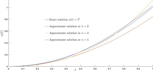
Figure 3. Error plots of Example 7.3 at different scale levels.

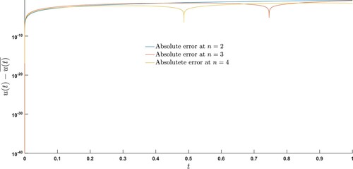
Figure 4. Exact and the approximate solutions of Example (7.4) are compared at various values of ${\beta }_1$.

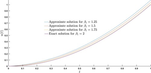
Figure 5. Exact and the approximate solutions of Example (7.5) are compared at different scale levels.

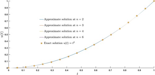
Figure 6. Exact and the approximate solutions of Example 7.2 are compared at n = 4, ${\beta }_1=3$, and ${\beta }_2=2.5$.

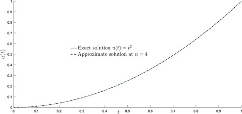
Table 5. Maximum absolute error of Example 7.4 at n = 10=scale level=number of terms of SLPs and for various choices of ${\beta }_1$.

t	${\beta }_1=1.25$	${\beta }_1=1.5$	${\beta }_1=1.75$	${\beta }_1=2$
0.0	$1.83\times {10}^{-40}$	$9.18\times {10}^{-41}$	$1.83\times {10}^{-40}$	0
0.2	$2.25\times {10}^{-2}$	$1.35\times {10}^{-2}$	$5.58\times {10}^{-3}$	0
0.4	$4.13\times {10}^{-2}$	$2.44\times {10}^{-2}$	$9.70\times {10}^{-3}$	0
0.6	$5.63\times {10}^{-2}$	$3.26\times {10}^{-2}$	$1.23\times {10}^{-2}$	0
0.8	$6.74\times {10}^{-2}$	$3.81\times {10}^{-2}$	$1.35\times {10}^{-2}$	0
1.0	$7.48\times {10}^{-2}$	$4.08\times {10}^{-2}$	$1.32\times {10}^{-2}$	0

Table 6. The Approximate solution of Example 7.5 is calculated at $n=\{2,3,4,6\}$=scale level=number of terms of SLPs, and for different values of t.

t	n = 2	n = 3	n = 4	n = 6
0.0	0.0000	0.0000	0.0000	0.0000
0.2	0.0424	0.0407	0.0401	0.0399
0.4	0.1632	0.1602	0.1598	0.1601
0.6	0.3626	0.3594	0.3599	0.3600
0.8	0.6405	0.6394	0.6403	0.6400
1.0	0.9969	1.0009	0.9998	1.0000

Table 7. Absolute error (AE) of Example 7.2 at $n=\{3,4\}$ = scale level= the number of terms of SLPs.

t	Exact solution	AE at n = 3	AE at n = 4
0	0	$1.4694\times {10}^{-39}$	$1.1615\times {10}^{-40}$
0.2	0.04	0	0
0.4	0.16	0	0
0.6	0.36	0	0
0.8	0.64	0	0
1.0	1.0	0	0

9. Conclusion

We proposed an approximate method to solve linear and nonlinear multi-order FDEs by extending the Paraskevopoulos's method for orthogonal SLPs. Our proposed method is based on decomposing the multi-order FDEs into a system of FDEs and then the resultant system is solved using the operational matrix approach. We checked the accuracy and efficiency of the method by solving various linear and nonlinear FDEs with constant and variable coefficients. We examined that with the increase of scale level, the approximate solutions were in a good agreement with the exact solutions. We also demonstrated the high efficiency of the method by determining the amount of absolute error and observed that as we increased the scale level, this amount was decreased significantly. It is important to note that only considering the few terms of SLPs, we obtained the satisfactory results. In addition, our proposed method has advantage to other methods, like Homotopy perturbation method, because in our case, the perturbation, linearization, or discritization are not necessary to be implemented. We also improved the numerically obtained results presented in [22]. Finally, our proposed method is fit to solve both linear and nonlinear problems of fractional order with constant and variable coefficients.

Acknowledgments

We thank the anonymous reviewers for their careful reading of our manuscript and their many insightful comments and suggestions which improve the quality of our manuscript.

Author's contributions

All authors contributed equally to this article. All authors read and approved the final manuscript.

Disclosure statement

The authors declare that they have no competing interests.

References

- Ahmed E, Elgazzar AS. On fractional order differential equations model for nonlocal epidemics. Physica A:Statistical Mechanics and its Applications. 2007;379(2):607–614.
- Sun H, Chen D, Zhang Y, et al. Understanding partial bed-load transport: experiments and stochastic model analysis. J Hydrol (Amst). 2015;521:196–204.
- Chen W, Sun H, Zhang X, et al. Anomalous diffusion modeling by fractal and fractional derivatives. Comput Math Appl. 2010;59(5):1754–1758.
- Sun H, Chen W, Chen Y. Variable-order fractional differential operators in anomalous diffusion modeling. Phys A. 2009;388(21):4586–4592.
- Kilbas A, Srivastava H, Trujillo J. Theory and application of fractional differential equations. New York (NY): Elsevier Science B.V.; 2006.
- Rossikhin Y, Shitikova M. Application of fractional derivatives to the analysis of damped vibrations of viscoelastic single mass systems. Acta Mech. 1997;120(1):109–125.
- Chen W. A speculative study of 2/3-order fractional Laplacian modeling of turbulence: some thoughts and conjectures. Chaos. 2006;16(2):023126.
- Agarwal R, Benchohra M, Hamani S. Boundary value problems for differential inclusions with fractional order. Adv Stud Contemp Math. 2008;12(2):181–196.
- Miller K, Ross B. An introduction to the fractional calculus and fractional differential equations. New York: Wiley; 1993.
- Podlubny I. Fractional differential equations. New York: Academic Press; 1998.
- Shah A, Khan R, Khan A, et al. Investigation of a system of nonlinear fractional order hybrid differential equations under usual boundary conditions for existence of solution. Math Methods Appl Sci. 2021;44(2):1628–1638.
- Tajadodi H, Khan Z, Irshad A, et al. Exact solutions of conformable fractional differential equations. Res Phys. 2021;22:1–6.
- Alshehri M, Duraihem F, Alalyani A, et al. A caputo (discretization) fractional-order model of glucose–insulin interaction: numerical solution and comparisons with experimental data. J Taibah Univ Sci. 2021;15(1):26–36.
- Bhrawy A, Zaky M. A fractional-order Jacobi Tau method for a class of time-fractional PDEs with variable coefficients. Math Methods Appl Sci. 2016;39(7):1765–1779.
- Mokhtaryand P, Ghoreishi F, Srivastava H. The Müntz-Legendre Tau method for fractional differential equations. Appl Math Model. 2016;40(2):671–684.
- Talib I, Belgacem FB, Asif NA, et al. On mixed derivatives type high dimensional multi-term fractional partial differential equations approximate solutions. In: AIP Conference Proceedings. Vol. 1798, No. 1. AIP Publishing; 2017.
- Khan RA, Khalil H. A new method based on Legendre polynomials for solution of system of fractional order partial differential equations. Int J Comput Math. 2014;91(12):2554–2567.
- Talib I, Tunc C, Noor ZA. New operational matrices of orthogonal Legendre polynomials and their operational. J Taibah Univ Sci. 2019;13(1):377–389.
- Doha E, Bhrawy A, Ezz-Eldien S. A new Jacobi operational matrix: an application for solving fractional differential equations. Appl Math Model. 2012;36(10):4931–4943.
- El-Sayed A, Baleanu D, Agarwal P. A novel Jacobi operational matrix for numerical solution of multi-term variable-order fractional differential equations. J Taibah Univ Sci. 2020;14(1):963–974.
- Heydari M, Atangana A, Avazzadeh Z, et al. An operational matrix method for nonlinear variable-order time fractional reaction diffusion equation involving Mittag–Leffler kernel. Eur Phys J Plus. 2020;135:237.
- Pak S, Choi H, Sin K, et al. Analytical solutions of linear inhomogeneous fractional differential equation with continuous variable coefficients. Adv Differ Equ. 2019;2019(256):1–22.
- Attar RE. Special functions and orthogonal polynomials. New York: Lulu Press; 2006.
- Mohammadi F, Hosseini M. A new Legendre wavelet operational matrix of derivative and its applications in solving the singular ordinary differential equations. J Franklin Inst. 2011;348(8):1787–1796.
- Saadatmandi A, Dehghan M. Numerical solution of a mathematical model for capillary formation in tumor angiogenesis via the Tau method. Commun Numer Methods Eng. 2008;24(11):1467–1474.