Accurate automatic classification system for 3D CT images of some vertebrate remains from Egypt

Abstract

Vertebrate fossils/remains became recently significant in various study fields for determining the ecological biodiversity. However, with the great abundance of fossils/remains and their classes, there is a difficulty in identifying and detecting these classes. Hence, in this paper, an accurate machine learning classification technique is presented to differentiate automatically some types of 3D vertebrate remain images. A computed tomography (CT) scanner is utilized to construct a dataset of 3D images of some vertebrate remains found in Egypt. Adaptive enhancement and segmentation processes are applied to the dataset. The different selected geometric features are then extracted. Thus, the extracted features are classified using suitable machine learning classifiers (SVM, KNN, DTs). The automatic detection for the remains class, according to the extracted features, is obtained using the confusion matrix for the training and testing data points and the receiver operating characteristic (ROC) curve. The results confirmed an accurate technique with high performance.

KEYWORDS:

• Machine learning (ML)
• vertebrate remains from Egypt
• K-nearest neighbour (KNN)
• decision tree (DT)
• support vector machine (SVM)
• features and segmentation

1. Introduction

Lately, paleontology is becoming a significant tool for obtaining qualitative and quantitative information about fossils and remains that enables an understanding of the evolution of the vertebrates [1,2]. These fossils include the remains of animals, bacteria, plants, fungi, and single-cell organisms that are preserved in the materials of the rocks [3]. Paleontology science plays a powerful role in detecting the extant and past biodiversity, describing the environmental changes in the past, studying the sensitivity of the ecosystem and detecting zoonosis [4]. In paleontology science, microscopic observations are considered among the accurate methods for the analysis and detection of the fossil types [5]. These analyses help to obtain geometric morphometrics and biological information about the tested fossils, but these may face great difficulty in determining fossil types [5,6]. This may be attributed to the differences in the abilities of examiners, especially the novice ones to distinguish the geometric morphometrics features of fossil skeletons [7,8]. In addition, the techniques that are used to perform the biological analysis are considered expensive and may not be available in all countries [6]. Consequently, it is important to introduce digital image processing and machine learning techniques to perform accurate and automatic classification for fossil types and for the digitalized library propose.

Digital image processing is a technique used to implement some statistical or mathematical operations on an image to retrieve and analyse some meaningful information from it or obtain an enhanced image [9,10]. The digital image processing techniques have many applications in different fields such as remote sensing, atmosphere study, medical field, feature extraction and others [10]. Image processing includes two essential operations: image enhancement and image segmentation [11,12]. The image enhancement aims to remove noise (denoising), enhance contrast and improve image quality compared to the original one [11]. Various filters such as Winner filter, medium filter and average filter are applied to remove the unwanted noise from the captured image [13]. In addition, in this stage, image enhancement algorithms like histogram equalization and linear contrast stretching may be utilized to improve the contrast of the captured image [14]. The second operation that is implemented on the enhanced image is the segmentation of the image. Generally, image segmentation can be defined as the process of partitioning the enhanced image into many segments in which each segment belongs to a signal object and its pixels are connected [15,16]. The main goal of the image segmentation techniques is to find the optimal threshold (T_opt) value of the image and then convert it to a binary image (1 for white and 0 for black) according to this value [10,15]. Many segmentation techniques have been proposed to perform this task. These techniques include Otsu's method [16], k-means clustering method, region-growing method and fuzzy c-means clustering algorithm [10].

Machine learning (ML) is formidable technique that utilizes computational approaches to obtain the usable model from empirical data points [17,18]. The ML is considered a subfield of artificial intelligence (AI) [19]. ML techniques can automatically progress and learn from their acquired experience without being punitively programmed [19,20]. ML has various applications in many fields such as classifying and recognizing the different classes in the enormous dataset, concepting the phenomenon of cyber that generated the data points under investigation, utilizing the generated models for predicting the future data point values and revealing the exhibited anomalous behaviour from data points under investigation [17–20]. Generally, the machine learning techniques are divided into two main types: supervised and unsupervised [18]. Supervised learning algorithms try to model relationships and dependencies between the target prediction output and the input features such that we can predict the output values for new data based on those relationships that it learned from the previous data sets [20,21]. They are used for predictive models and for labelled data. Regression and classification are the main types of supervised learning problems. The most commonly used algorithms are nearest neighbour, decision trees, linear regression, support vector machines (SVMs) and neural networks (NNs).

Unsupervised learning is mainly used in pattern detection and descriptive modelling [20]. These algorithms can try to model relationships between the output categories or labels, so, these techniques try to use processes on the input data to mine the rules, detect patterns, and summarize and group the data points. This helps the user to derive meaningful insights and describe the data [21,22]. The main types of unsupervised learning algorithms are k-means clustering and association rules [22]. One of the important digital image processing and machine learning applications occurs in paleontology [22–28].

Many authors have used convolutional neural networks (CNNs) to identify the species of fossils and remains [22–29]. Pedraza et al. [22] utilized pre-trained AlexNet for detecting diatom classes. Rehn et al. [23] applied the Visual Geometry Group 16 (VGG16) network for classifying the particles of charcoal. Carvalho et al. [24] applied U-NET to perform segmentation for planktonic microorganisms. Johansen and Sørensen utilized the pre-trained VGG16 network for identifying foraminifera types [29].

The present study processed the 3D CT images of three vertebrate remains collected from Egypt, representing the skull of a crocodile from the ancient deposits of Lake Qarun of the Fayum Depression, the skull of a dolphin that died 3 years ago on the beach near the Damietta city and a fragment of hippopotamus maxilla (jaw) from the ancient delta deposits in Kafr El Sheikh governorate.

2. Problem formulation

The majority of the studies utilized the convolutional neural networks for performing their classification tasks on two-dimensional (2D) images. The usage of the 2D images gives restricted information about the structure of the acquired fossils/remains, which may lead to an inaccurate investigation of the fossils and remains [30]. In addition, the extracted features may be vague for researchers, which may influence especially time of need for some explanations according to the CNN. Owing to extracting the features occurs directly and automatically using the convolution layers of the network from the inserted image. It is to be noted that, there are few studies available in the literature that have studied this type of fossils/remains.

Therefore, the main goal of the current study is to present an accurate classification system to differentiate automatically some types of 3D CT images for vertebrate remains/fossils. For this study, 3D dataset images of the remains under study are constructed using the CT scanner that provides more details about the structure of the remains. The digital image processing techniques are used to extract defined features for the remains and then send these features to some machine learning classifiers. To evaluate the efficiency of the automatic classification system, the F1 score and the receiver operating characteristic (ROC) curve measures are determined.

3. Proposed method

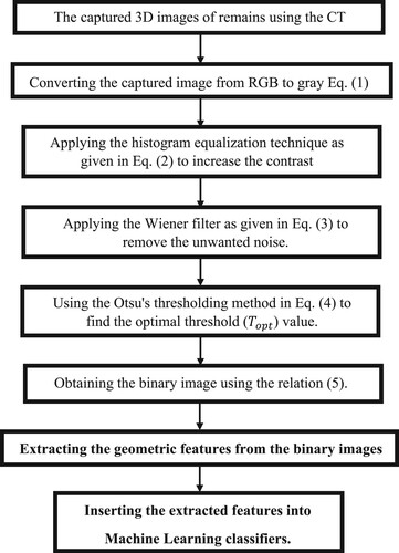
A method is suggested to detect accurately some vertebrate remains types using a classification system. A schematic diagram for the proposed method is shown in Figure 1 that is performed through the following steps.

Figure 1. Schematic diagram for the proposed method.

3.1. Dataset establishment (Data acquisition)

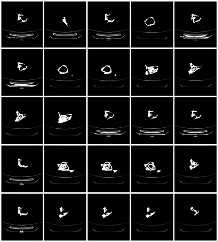
In this work, a computed tomography (CT) scanner of version 128 Slice GE Optima is used to generate a 3D image dataset for three classes of remains, which are a crocodile head, a dolphin head and a part of hippopotamus maxilla (see Figure 2). During a CT scan, each vertebrate remain is mounted on a table inside the tunnel of the CT machine and a series of X-rays images were taken from different angles. This procedure is repeated on different vertebrate remains. Each 3D image in this dataset is acquired by recording a 1D projection at different angles from 1^o to 360^o. Then, reconstructed 3D images from these projections using the filtered back projections technique [31]. To our knowledge, this is an early established dataset for these types of remains. This dataset includes (2052) 3D images for three main classes: crocodile head (820 images), dolphin head (653 images) and a part of a hippopotamus maxilla (579 images). These images have a resolution of 512×512×3 with a 24-bit colour depth. The dataset images are divided into 1912 images for training and 140 images for the evaluation of the results. Figures 3–5 show examples of the recorded 3D images dataset that includes the crocodile head, dolphin head and the hippopotamus-maxilla part, respectively.

Figure 2. Examples for 3D visualization for the tested remains. (a) Crocodile head, (b) dolphin head and (c) part of hippopotamus-maxilla.

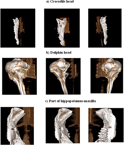
Figure 3. Examples for the recorded 3D image dataset of the crocodile skull.

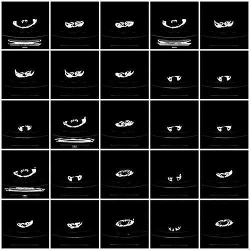
Figure 4. Examples for the recorded 3D image dataset for the dolphin skull.

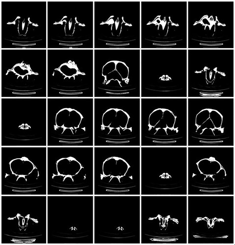
Figure 5. Examples for the recorded 3D image dataset for the hippopotamus maxilla.

3.2. Preprocessing process

In this step, the captured RGB image is converted into a greyscale image $G\left(x,y\right)$ using the NTSC formula as described by the following equation [10] (1) $G\left(x,y\right)=0.299\ast R+0.587\ast G+0.114\ast B$(1) where R, G and B represent the channels of red, green and blue colours, respectively, in the image. Then, the histogram equalization technique is applied to the obtained image in Equation (1) to improve its contrast as given in the following equation [10] (2) $H=\sum _{i=1}^m\frac{f_i}{f}\left(Z-1\right)$(2) where $m$ is the intensity range of the $G\left(x,y\right)$ image, $f_i$ presents the frequency of intensity $i$, $f$ refers to the sum of all the frequencies and $Z$ presents total grey levels of the output image. To remove the unwanted noise (denoising), the Wiener filter ($W_u\left(u_x,u_y\right)$) is applied as shown in the following equation [10,13]: (3) $W_u\left(u_x,u_y\right)=\frac{S^{\ast }\left(u_x,u_y\right)}{{|U\left(u_x,u_y\right)|}^2+\frac{{\text{β}}_n\left(u_x,u_y\right)}{{\text{β}}_s\left(u_x,u_y\right)}}$(3) where $S\left(u_x,u_y\right)$ and $S^{\ast }\left(u_x,u_y\right)$ are the noise function and its complex conjugate in the frequency domain$\left(u_x,u_y\right)$, respectively, and .. and ${\text{β}}_s$ are the spectral strength for the unwanted noise and signal, respectively.

3.3. Segmentation process

To extract the needed properties from the dataset images, the binary image is required. To perform this task, we can use Otsu’s thresholding method as a suitable algorithm to find the global threshold ($T_{opt}$) value. This algorithm is based on finding the weighted sum of variances of the two classes as described in the following equation [16]: (4) ${\sigma }_w^2\left(T\right)=w_1{\sigma }_1^2\left(T\right)+w_2{\sigma }_2^2\left(T\right)$(4) where $w_1\mathrm{\&}{w}_2$ present the probabilities of the two classes separated by a threshold$T$, and ${\sigma }_1^2\mathrm{\&}{\sigma }_2^2$refer to the variances of the two classes.

Here, the threshold that minimizes the intra-class variance of the two classes is considered the optimal threshold ($T_{opt}$). According to the value of $T_{opt}$, the binary image can be obtained using the following relation [16]: (5) $G\left(x,y\right)=\{\begin{array}{ll}1\left(white\right),& \text{for each pixel}\ge T_{opt}\\ 0\left(black\right),& \text{for each pixel}<T_{opt}\end{array}$(5)

3.4. Feature extraction and classification

The feature extraction process is considered key to any successful classification. This is because the extracted features are the main parameters to differentiate between the classes in the dataset images. Many types of features can be extracted from images according to the conditions of the study and the nature of the tested objects. These features include colour features, statistical features, geometric features and texture features [32]. In the present study, the geometric features would be recommended and more suitable for acquired vertebrate remains due to the ability for analyzing this data type with more details compared to the other types of features. This is because the classification of vertebrate fossils is based primarily on the geometric shape of the bones of these fossils, so the geometric characteristics are considered the dominant features to classify these fossils.

Figure 6. Step-wise visual output for the extraction features.

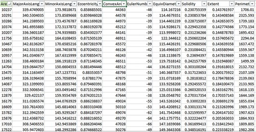
Figure 7. (I) Confusion matrix of the trained data using the quadratic SVM classifier. (II) ROC curve of the trained data point using the quadratic SVM classifier. (III) Confusion matrix of the testing data via the quadratic SVM classifier.

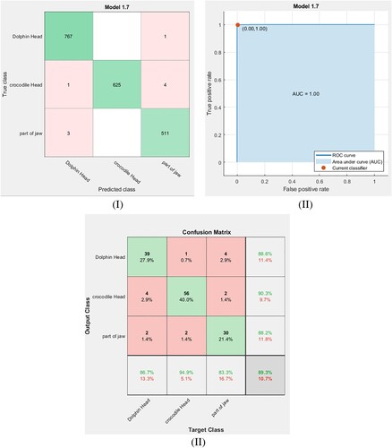
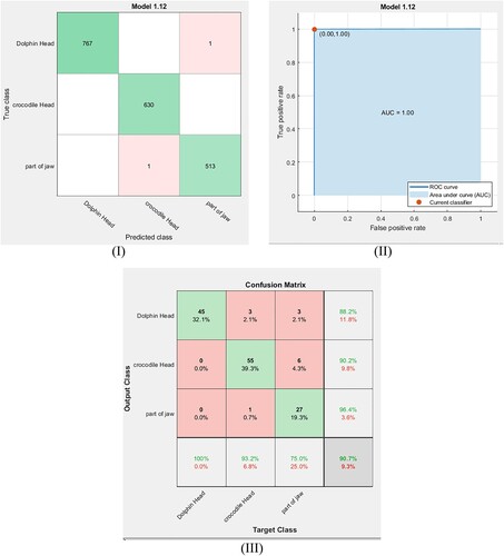
Figure 8. (I) Confusion matrix of the trained data by the cubic SVM classifier. (II) ROC curve for the trained data by the cubic SVM classifier. (III) Confusion matrix of the testing data via the cubic SVM classifier.

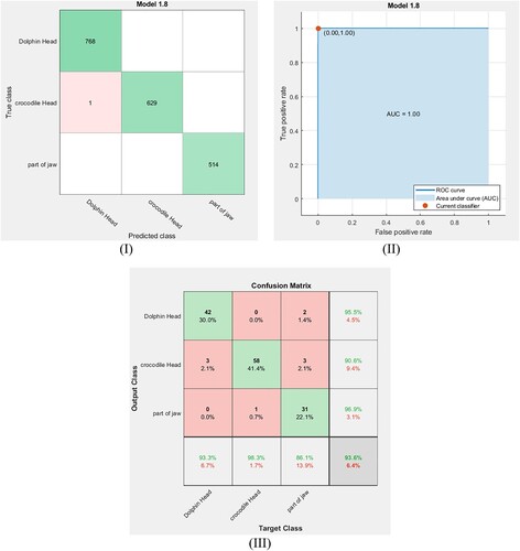
Figure 9. (I) Confusion matrix of the trained data by the fine Gaussian SVM classifier. (II) ROC curve of the trained data by the fine Gaussian SVM classifier. (III) Confusion matrix of the testing data point by the fine Gaussian SVM classifier.

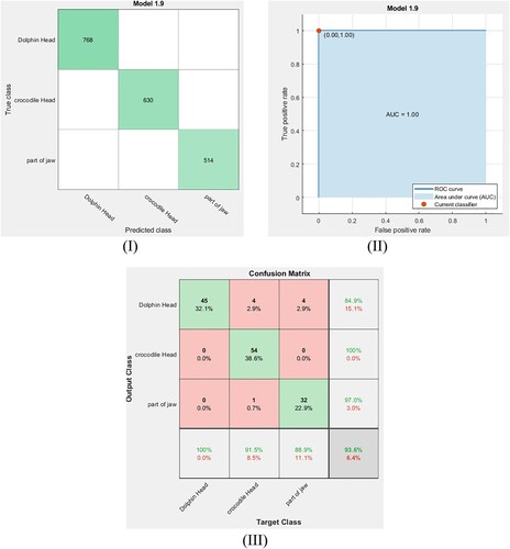
Table 1. Training and testing accuracy rates for each used model with their F1 score and training times.

Trained model	Accuracy of training (%)	Time of training (s)	Accuracy of testing (%)	F1 score
Quadratic SVM	99.53	1.3171	89.29	0.89
Cubic SVM	99.95	1.0206	93.57	0.93
Fine Gaussian SVM	100	1.2476	93.57	0.9366
Fine KNN	99.9	1.2325	90.71	0.90
Fine DT	98.33	6.451	88.57	0.88
Medium DT	95.87	0.33744	86.43	0.85
NN	96.6	1.672	92.02	0.919

In this work, many geometric features are extracted from the obtained binary images in Equation (5) to perform a classification for the classes in our dataset. These features include (1) the area of the skeleton that can be defined as the number of pixels in the skeleton, (2) the convex area that is the convex hull area enclosing the skeleton, (3) solidity that can be defined as the ratio between the area of the skeleton and the convex area of the skeleton, (4) major axis of the skeleton that is the endpoints of the longest line that can be drawn through the skeleton, (5) minor axis of the skeleton that is the endpoints of the longest line that can be drawn through the skeleton whilst remaining perpendicular with the major axis, (6) eccentricity that can be defined as the ratio between the length of the minor (short) axis and the length of the major (long) axis of an object, (7) the Euler number that is defined as the total number of objects in an image minus its total number of holes, so we can use the Euler number to detect all holes and vacuoles inside the vertebrate fossils, which helps to raise the classification efficiency, and (8) the perimeter of the skeleton that is the number of pixels in the boundary of the skeleton [33] are taken into account for the features. Figure 6 shows a step-wise visual output for the extraction features. After extracting these features from the images in our dataset, the features are sent to some machine learning classifiers to train and test them to complete the classification process.

4. Results and discussions

According to the proposed method, the images in our dataset are converted to greyscale images using Equation (1). Then, to increase the dynamic range of the images of our dataset we applied the histogram equalization technique as given in Equation (2). Also, to remove the unwanted noise we applied the Wiener filter as expressed in Equation (3). After detecting the optimal threshold ($T_{opt}$) values for the images using Equation (4), the relation in Equation (5) is used for obtaining the binary images for our dataset. The geometric features of the remains in the obtained binary images are extracted using the designed Matlab program. Now, the extracted features become ready for the training and classification processes. Each ML algorithm is not run separately for each feature but for the whole extracted features simultaneously. The classification results are not a mean of the partial results; however, they are the result of running for all features simultaneously.

4.1. Classification process using the support vector machine (SVM) classifier

The support vector machine (SVM) is considered among the most robust supervised learning methods [17,34]. This classifier has a high capacity for learning and reducing error sources, driving to effectively differentiate the classes of data points, especially the imbalanced data [18]. The basic principle of this classifier is based on converting the recoded data points from the recording space into higher dimensional feature space using a non-linear mapping function and then generating boundaries (hyperplanes) with a maximum margin of separation for the data points classes [20]. The most common mapping function used in the SVM classifiers includes linear SVM, quadratic SVM, cubic SVM, fine Gaussian SVM, medium Gaussian SVM and coarse Gaussian SVM.

For the current dataset, SVM classifiers with quadratic, cubic and fine Gaussian kernels are used to detect the remains class in our dataset. These classifiers are optimized with cross-validation equal to 5-fold. Then, the data points (features) are trained via these classifiers. To determine the accuracy of the training process using these classifiers, the confusion matrix is used. Figures 7(I), Figure 8(I) and Figure 9(I) show the confusion matrix for the training dataset using the quadratic SVM, the cubic SVM and the fine Gaussian SVM classifiers, respectively. From these confusion matrices, the accuracy of training is calculated using the following equation [35]: (6) $\text{Accuracy}=\frac{\text{TP}+\text{TN}}{\text{TP}+\text{TN}+\text{FP}+\text{FN}}$(6) where TP, TN, FN and FP are the true positive, true negative, false negative and false positive values, respectively. The obtained results are given in Table 1. Also, the receiver operating characteristic (ROC) curve is used to assess the performance of the training process at all classification thresholds. Figure 7(II), Figure 8(II) and Figure 9(II) show the ROC curves for the training dataset using the quadratic SVM, the cubic SVM and the fine Gaussian SVM classifiers, respectively. Here, the ROC curves are plotted by finding the relation between the true positive rate (TPR) known as sensitivity and the false positive rate (FPR) known as specificity at all classification thresholds [35]. The obtained results in Figure 7(III), Figure 8(III) and Figure 9(III) illustrate that the points determined by TPR and FPF on ROC curves for the three SVM classifiers are at (0, 1) and the area under curves are found to be 1 and these results represent the ideal situation of the identification in which these classifiers have a specificity of 100% and a sensitivity of 100%. This indicates that these classifiers are optimum models for the identification of the present remains class.

After exporting and saving these classifier models, 140 images are used to test these models. The confusion matrixes for the tested dataset using the quadratic SVM, the cubic SVM and the fine Gaussian SVM classifiers are shown in Figure 7(III), Figure 8(III) and Figure 9(III), respectively. From these figures, the accuracy of testing for each classifier is calculated using Equation (1), and the results are listed in Table 1. Furthermore, the F1 score is calculated from the obtained confusion matrix, to assess the performance of the testing process for each model, using the following relation and the outcome results are given in Table 1. F1 score values are taken from 1 (the perfect case) to 0 (the worst one) [35]. (7) $\text{F}1\text{ score }=\frac{2\left(\text{Precision}\ast \text{Recal}\right)}{\text{Precision}+\text{Recal}}$(7)

4.2. Classification process using the K-nearest neighbour (KNN) classifier

The K-nearest neighbour (KNN) classifier is a non-parametric and laziest learning algorithm [34]. The fundamental behind this classifier is based on utilizing the distance functions and similarity measurements to find k-nearest data points in a data set via applying the majority voting over the classes of these data points [36,37]. The most common distance functions that are used in the KNN classifiers include the normalized Euclidean metric, chi-square, Minkowski distance, Manhattan distance and cosine distance [37]. According to the rule of thumb, the k-values are selected to be odd numbers [34].

For the current dataset, the extracted features of remains are trained using the fine KNN classifier. Here, the normalized Euclidean metric is used as a distance function with cross-validation folds equal to 5-fold. Figure 10(I, II) shows the confusion matrix and ROC curve for the training dataset using the fine KNN classifier. Using Equation (6), the accuracy of the training for this classifier is calculated from Figure 10(I), and the result is reported in Table 1. The verified point by TPR and FPF for the obtained ROC curve in Figure 10(II) is (0, 1), and this is a signal for this classifier is an optimal model for the identification. After exporting and saving this classifier model, the same small dataset is used to test the exported model. Figure 10(III) shows the confusion matrix for the tested dataset using the fine KNN classifier. From Figure 10(III), the accuracy of testing and the F1 score are calculated for this classifier system, and the results are listed in Table 1.

Figure 10. (I) Confusion matrix of the trained data via the fine KNN classifier. (II) ROC curve of the trained data via the fine KNN classifier. (III) Confusion matrix of the testing data via the fine KNN classifier.

4.3. Classification process using the decision tree (DT) classifier

The decision tree is a supervised learning algorithm that used the tree structure to perform the classification process [37]. In DT, the tree is constructed from the data points of the dataset and then divided into smaller subsets (root nodes and leaf nodes) until no more dividing can be performed [38]. The main goal of the DT classifier is to generate a training model for predicting the classes in a dataset. To perform this task, we begin from the root of the tree and then the root attribute values are compared with the record’s attribute [37,38]. On the premise of comparison, we keep track of the branch identical to that values and jump to the following node [38]. The most common DTs used in the classification process are fine tree, medium tree, and coarse tree.

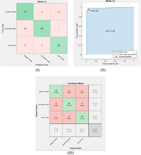
In the same manner, fine DT and medium DT classifiers are used to classify the fossil classes in our dataset with cross-validation equal to 5-fold. The extracted features are trained via these classifiers. Figure 11(I, II) and Figure 12(I, II) show the confusion matrix for the training dataset and their ROC curves using the fine DT and the medium DT classifiers, respectively. The obtained ROC curves in these figures clarify that the point determined by TPR and FPF for the fine DT classifier (Figure 11 (II)) is at (0.01, 0.98) and the point determined for the medium DT classifier (Figure 12(II)) is at (0.03, 0.95). This means that these classifiers have high accuracy but are not optimal for the present data. The accuracy rates of training for these classifiers are calculated using Equation (6) and the results are listed in Table 1. After exporting these classifier models, the same small dataset is used to test them. Figure 11(III and III) show the confusion matrix for the tested dataset using the fine DT and medium DT classifiers. From these figures, the accuracy of testing and the F1 scores are calculated for each classifier system and the results are reported in Table 1. To provide a broader view of performance for our dataset, the feed-forward back propagation neural network is utilized for training and classifying the considered classes. Hence, the result accuracy rates of the classification, the training time and the F1 score value for the ANN model are listed in Table 1.

Figure 11. (I): Confusion matrix for the trained data point via the fine DT classifier. (II) ROC curve for the trained data point via the fine DT classifier. (III) Confusion matrix for testing data point via the fine DT classifier.

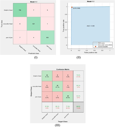
Figure 12. (I) Confusion matrix of the trained data using the medium DT classifier. (II) ROC curve of the trained data using the medium DT classifier. (III) Confusion matrix of the testing data using the medium DT classifier.

For the abovementioned classifiers, we conducted a permutation between the extracted features to select the best features for the training process. So, the obtained results in Table 1 are not the whole evaluated results, but the best selected features for the training and tested features.

In general, Table 1 clarifies that the cubic SVM and fine Gaussian SVM classifier system based on the extracted geometric features have a high efficiency (highest testing accuracy) in classifying and detecting the remains class compared to the other classifier systems. In addition, F1 score values refer that the SVM classifier system with fine Gaussian kernel (F1 score = 93.66%) has the highest performance for classifying the remains class. Actually, the fine Gaussian SVM with 100% accuracy of training means that the model is overfitting; therefore, we will consider the cubic SVM to perform the required classification to avoid this overfitting. In other words, the SVM with fine Gaussian kernel is not outperforming compared to other approaches and its high accuracy result may be attributed to overfitting occurrence during training of the model. So, we will exclude it from our consideration. Hence, the cubic SVM classifier is considered the dominant classifier in our study.

5. Conclusions

An accurate classification system has been developed to differentiate automatically some types of 3D vertebrate remains images, which are a crocodile head, a dolphin head, and a part of the hippopotamus maxilla that are discovered in Egypt. The used images of the remains are 3D dataset images, which are constructed using the computed tomography (CT) scanner that can support more details about the structure of the remains. The preprocessing techniques are used to remove the noise and improve the contrast of the images. The histogram equalization technique and Wiener filter are used. Otsu's thresholding method is utilized to obtain the binary images for the constructed remains dataset. The suitable selected geometric features are extracted. Classification ML techniques based on SVM, KNN, NN and DT models are utilized to classify these remains classes automatically. Efficiency evaluation for these classification systems is performed via confusion matrix, F1 score value, and the ROC curve. The obtained results show that the SVM classifier system with a cubic kernel has the highest performance for classifying the fossil classes. In addition, it may be used as an efficient classifier tool for remains classification. Hence, the proposed method shall be used as an efficient diagnostic tool for geologists or paleontologists.

Acknowledgments

The authors are grateful to the reviewers for their valuable comments and thank Prof Dr Hesham Sallam, the Founder and Director of Mansoura University Vertebrate Paleontology Center, for the appreciated cooperation regarding the fossile/remain samples. In addition, the authors would like to express their gratitude to Dr Emam Z. Omar for his help in building the ML system, and appreciating the efforts of the reviewers for their valuable comments that improved the paper.

Disclosure statement

No potential conflict of interest was reported by the author(s).

References

- Saraswati PK, Srinivasan M. Micropaleontology: principles and applications. Cham: Springer; 2016, pp. 35–77.
- Cucchi T, Mohaseb A, Peigné S, et al. Detecting taxonomic and phylogenetic signals in equid cheek teeth: towards new palaeontological and archaeological proxies. R Soc Open Sci. 2017;4(4):160997.
- Cucchi T, Papayianni K, Cersoy S, et al. Tracking the near western origins and European dispersal of the western house mouse. Sci Rep. 2020;10(8276):8276–8288.
- Müller L, Gonçalves GL, Cordeiro-Estrela P, et al. DNA barcoding of sigmodontine rodents: identifying wildlife reservoirs of zoonoses. PLoS One. 2013;8(11):e80282–e80294.
- Flügel E. Microfacies of carbonate rocks: analysis, interpretation and application. 2nd ed. Berlin: Springer; 2010.
- Salonen JS, Korpela M, Williams JW, et al. Machine-learning based reconstructions of primary and secondary climate variables from north American and European fossil pollen data. Sci Rep. 2019;9:15805.
- Adams CD, Otarola-Castillo E. Geomorph: an R package for the collection and analysis of geometric morphometric shape data. Methods in Ecology and Evolution. 2013;4:393–399. DOI: 10.1111/2041-210X.12035.
- Barčiová L, Macholán M. Morphometric key for the discrimination of two wood mice species, Apodemus sylvaticus and A. flavicollis. Acta Zool Acad Sci Hung. 2009;55(1):31–38.
- Kuruvilla J, Sukumaran D, Sankar A, et al. A review on image processing and image segmentation. International conference on data mining and advanced computing (SAPIENCE), Ernakulam, India, 2016. pp. 198–203.
- Gonzalez RC, Woods RE. (2018). Digital image processing. Global Edition. Pearson Education Limited.
- Al-Tahhan FE, Sakr AA, Aladle DA, et al. Improved image segmentation algorithms for detecting types of acute lymphatic leukemia. IET Image Proc. 2019;13(13):2595–2603.
- Zheng J, Zhang D, Huang K, et al. Image segmentation framework based on optimal multi-method fusion. IET Image Proc. 2019;13:186–195.
- Omar EZ. A refined denoising method for noisy phase-shifting interference fringe patterns. Opt Quantum Electron. 2021;53 1–24.
- Kim YT. Contrast enhancement using brightness-preserving bi-histogram equalization. IEEE Trans. Consum Electron. 1997;3:1447–1453.
- Karthikeyan T, Poornima N. Microscopic image segmentation using fuzzy C means for leukemia diagnosis. Int J Adv Res Sci Eng Technol. 2017;4:3136–3142.
- Otsu NA. Threshold selection method from gray-level histograms. Automatica. 1975;11:62–66.
- Kotsiantis SB. Supervised machine learning: a review of classification techniques. Informatica . 2007;31:249–268.
- Paluszek M, Thomas S. MATLAB machine learning. Princeton (NJ): Apress; 2017.
- Bousquet O, Boucheron S, Lugosi G. Theory of classification: a survey of recent advances. ESAIM Probab. Stat. 2005;9:249–268.
- Al-Tahhan FE, Fares ME, Sakr AA, et al. Accurate automatic detection of acute lymphatic leukemia using a refined simple classification. Microsc Res Tech. 2020;83:1178–1189.
- Omar EZ. Investigation and classification of fibre deformation using interferometric and machine learning techniques. Appl Phys B. 2020;126:1–14.
- Pedraza A, Bueno G, Deniz O, et al. ‘Automated diatom classification (part B): a deep learning approach. Appl Sci. 2017;7:460.
- Rehn E, Rehn A, Possemiers A. Fossil charcoal particle identification and classification by two convolutional neural networks. Quaternary Sci. Rev. 2019;226:106038.
- Carvalho LE, Fauth G, Fauth SB, et al. (2019). Automated microfossil identification and segmentation using a deep learning approach. DOI:10.1016/j.marmicro.2020.101890.
- Dey N, Rajinikanth V, Shi F, et al. Social-group-optimization based tumor evaluation tool for clinical brain MRI of flair/diffusion-weighted modality. Biocybern Biomed Eng. 2019;39:843–856.
- Moraru L, Moldovanu S, Traian Dimitrievici L, et al. Gaussian mixture model for texture characterization with application to brain DTI images. J Adv Res. 2019;16:15–23.
- Moldovanu S, Obreja C-D, Biswas KC, et al. Towards accurate diagnosis of skin lesions using feedforward back propagation neural networks. Diagnostics. 2021;11:1–16.
- Moldovanu S, Toporaş LP, Biswas A, et al. Combining sparse and dense features to improve multi-modal registration for brain DTI images. Entropy. 2020;22:1–16.
- Haugland Johansen T, Aagaard Sørensen S. Towards detection and classification of microscopic foraminifera using transfer learning; 2020.
- Hou Y, Cui X, Canul-Ku M, et al. ADMorph: a 3D digital microfossil morphology dataset for deep learning. IEEE Access. 2020;8:148744–148756.
- Bevins N, Zambelli J, Li K, et al. Multicontrast x-ray computed tomography imaging using talbot-Lau interferometry without phase stepping. Med Phys. 2012;39(1):424–428.
- Murugappan M, Mutawa A. Facial geometric feature extraction based emotional expression classification using machine-learning algorithms. PLOS ONE. 2021;16:1–20.
- Omar EZ, Sokkar TZN, Hamza AA. In situ investigation and detection of opto-mechanical properties of polymeric fibres from their digital distorted microinterferograms using machine learning algorithms. Opt Laser Technol. 2020;129:1–16.
- Purwanti E, Evelyn C. Detection of acute lymphocyte leukemia using k-nearest neighbor algorithm based on shape and histogram features. J Phys. 2017;853:1–5.
- Gates G. The reduced nearest neighbor rule. IEEE Trans Inf Theory. 1972;18:431–433.
- Patel HH, Prajapati P. Study and analysis of decision tree based classification algorithms. Int J Comput Sci Eng. 2018;16:74–78.
- Sharma H, Kumar S. A survey on decision tree algorithms of classification in data mining. Int J Sci Res. 2016;5:2094–2097.
- Zhong Y. The analysis of cases based on decision tree. 7th IEEE International conference on software engineering and service Science (ICSESS), Beijing, China, 2016.