Influence of activation energy on triple diffusive entropy optimized time-dependent quadratic mixed convective magnetized flow

Abstract

The flow over a wedge with activation energy and chemical reaction gains widespread applications in compound creations, food processing, insulation, oil reservoirs, catalysis, etc. The vast applicability of activation energy with a binary chemical reaction comprising multiple diffusions and the time-dependent nature of the entropy-optimized flow has drawn our attention to this work. The consequences of time, activation energy, liquid hydrogen and oxygen diffusions, and magnetic field over a wedge in the quadratic combined convection flow with entropy analysis are explored to achieve more mechanically realistic outcomes. The nonlinear dimensional coupled partial differential equations (PDEs) that govern the modelled phenomenon are tackled with non-similar transformations, the Quasilinearization technique followed by an implicit finite difference scheme and Varga’s matrix inverse procedure. The entropy generation can be minimized by upsurging the magnitude of the temperature difference ratio attribute ${\mathrm{\Omega }}_T$. The higher wedge angle results in a lower fluid motion.

KEYWORDS:

• Unsteady flow
• entropy generation
• activation energy
• Quasilinearization technique
• finite difference scheme
• quadratic combined convection

Nomenclature

$x,y$	=	Cartesian coordinates
$u,v$	=	$x$ and $y$ velocity components
$U_e$	=	Mainstream velocity
$U_{\mathrm{\infty }}$	=	Mainstream velocity constant
$C_j$	=	Species concentration
$C_p$	=	Specific heat
$T$	=	Fluid temperature
$T_w$	=	Wall temperature
$t$	=	Time
$f$	=	Nondimensional stream function
$T_{\mathrm{\infty }}$	=	Ambient fluid temperature
$F=f_{\eta }$	=	Nondimensional velocity
$G$	=	Nondimensional temperature
H, S	=	Dimensionless species concentration of liquid hydrogen and oxygen
K	=	Thermal conductivity
$D_{s_j}$	=	Mass diffusivity
$N{c}_1,N{c}_2$	=	Buoyance ratio parameters for liquid hydrogen and oxygen
$g$	=	Acceleration due to gravity
$Ri$	=	Richardson number
$Pr$	=	Prandtl number
$S{c}_j$	=	Schmidt number
$R^{\ast }$	=	Gas constant
$C_{fx}$	=	Local surface drag coefficient
$N{u}_x$	=	Local strength of heat transfer
$S{h}_{jx}$	=	Local strength of mass transfer
Br	=	Brinkman number
Be	=	Bejan number
$M_i$	=	Diffusion parameters
$n_1,n_2$	=	liquid hydrogen & oxygen rate constants
$E_{a_1},E_{a_2}$	=	Activation energy for liquid hydrogen & oxygen
$K_{r_1},K_{r_2}$	=	Chemical reaction rate constants for liquid hydrogen & oxygen
$K{c}_1,K{c}_2$	=	Chemical reaction parameters
$E_1,E_2$	=	Activation Energy parameter for liquid hydrogen and oxygen
$m$	=	Wedge angle parameter
$\mathrm{\Omega }$	=	Wedge angle
$M$	=	Magnetic parameter
$B$	=	Constant magnetic field strength
$\overline{x}$	=	Dimensional axial distance

Greek symbols

$\psi$	=	Stream function
$\xi ,\eta$	=	Transformed variables
${\text{β}}_1,{\text{β}}_2$	=	linear and quadratic thermal expansion coefficients
${\text{β}}_3,{\text{β}}_4$	=	Liquid hydrogen's linear and quadratic concentration expansion
coefficients	=
${\text{β}}_5,{\text{β}}_6$	=	Liquid oxygen's linear and quadratic concentration expansion

Coefficients

$\tau$	=	Nondimensional time
$\alpha$	=	Unsteady parameter
$\varphi \left(\tau \right)$	=	Unsteady function of $\tau$
$\kappa$	=	Boltzmann constant
${\text{β}}_t$	=	Quadratic convection parameter for temperature
${\text{β}}_{c_1}$	=	Nonlinear convection parameter for liquid hydrogen
${\text{β}}_{c_2}$	=	Nonlinear convection parameter for liquid oxygen
${\mathrm{\Omega }}_T$	=	temperature difference ratio
${\mathrm{\Omega }}_{c_1}$	=	liquid hydrogen concentration difference ratio
${\mathrm{\Omega }}_{c_2}$	=	liquid oxygen concentration difference ratio

Subscripts

$\xi ,\eta$	=	Partial derivatives with respect to $\xi ,\eta$
$w,\mathrm{\infty }$	=	at the surface and away from the surface, respectively

1. Introduction

Svante Arrhenius, a Swedish scientist introduced the Activation Energy (AE) concept for the first time in 1889. The minimum energy the chemical species requires to instigate a chemical reaction is known as the AE. The AE is different for different chemical reactions and may be zero for some chemical reactions. Bestman [1] was probably the first to work on a binary chemical reaction with AE. Numerous industrial applications involve binary chemical reactions with AE. Examples are geothermal artificial lake retrieval, atomic reaction rotting, food processing, insulation, oil reservoirs, compound creations, catalysis, thermal lubricant retrieval, ceramics production, biochemical systems, and many more. Given these numerous applications, many researchers [2–10] have worked on this concept of AE. Dhlamini et al. [2] have discussed the effects of AE and convective boundary conditions over an infinitely long plate. They concluded that AE enhances the concentration profile significantly. Ali et al. [3] explored the AE on the 3D flow of cross nanofluid. The effect of AE, thermal radiation, and entropy generation in a quadratic combined convective flow of nanofluid was investigated by Alsaadi et al. [4].

Triple (multiple) diffusion flows can be achieved by taking the temperature diffusion with two different species or considering three different diffusing species. The stratospheric warming, underground water flow, food processing, etc., involves multiple diffusions. There are very limited studies on triple diffusion [11–14]. Since the process of AE can be seen in a binary chemical reaction, one can confine the binary reaction by employing a particular species concentration to attain more perfection in the results. For example, liquid hydrogen, liquid oxygen, etc., can be taken as a particular species concentration. In the space programme, liquid hydrogen is used in enormous quantities as a major rocket fuel for oxygen combustion and cooling the aircraft engine. In the propellant systems of missiles and rockets, liquid oxygen is an oxidant for liquid fuels. By incorporating diffusions of specific species namely liquid hydrogen and oxygen, activation energy applications can be expanded.

Each and every flow in nature and industry is connected with time, and time has a very significant impact on the thermal engineering properties [15–19]. Unsteady or time-dependent [20–23] flow problems are vital in many engineering disciplines. For example, the interaction of rotating and stationary parts in a piston engine, turbomachinery, helicopter aerodynamics, etc. Many academicians do not focus on unsteady flow problems because of their difficulties, despite their applications. However, very recently, Noor et al. [20], Jenifer et al. [21], and Daniel et al. [22] have examined the unsteady flow nature over different geometries and concluded that velocity declines for improving values of the unsteadiness parameter.

The entropy, a thermodynamic function, embodies the system's functioning status. Inability of a system to transfer thermal energy into mechanical energy is known as “Entropy”. Entropy generation (EG) must be kept to a minimum for engineering systems to function well. For example, air-conditioning systems, heat exchangers, fuel cells, units of thermal power stations, etc. to work efficiently. Bejan [24] was the one who proposed the concept of EG in 1982 for the first time. Several works were made by considering the analysis of EG [25–27] and the effect of AE over the period [4, 6,7]. The results reveal that for higher Brinkman numbers, EG is enhanced for forced convection when there is a significant magnetic field. Due to the significant impact of EG in engineering, it is very important to minimize the EG in the system.

Studies over a wedge attracted researchers due to its significant applications in aerospace, pharmaceuticals, oil and gas industries, thermal insulation, dams, designing of disks for engine gate valves etc. Owing to these important industrial applications, some researchers [28–35] discussed the impact of different effects on the wedge. Watanabe et al. [28] solved the problem on a wedge with uniform suction /injection using the difference-differential method. By using magnetohydrodynamics (MHD), Kafoussias and Nanousis [29] extended Watanabe et al. ‘s [28] investigation and demonstrated that a magnetic field slows the fluid's velocity. The non-similarity solution to the wedge with the unsteady flow in a bi-convective region was given by Singh et al. [30]. A work on a wedge was conducted by Kumari et al. [31] in a porous medium. These studies are restricted to only similarity solutions. The overshoot in the velocity due to buoyancy reduces for increasing time. This study is then protracted to account for non-uniform slot injection/suction by Ganapathirao et al. [32].

The temperature and concentration variance in the flow around a wedge at a high temperature will not be linear in most cases. So, one has to overcome this difficulty by involving nonlinear (quadratic) combined convection [4–6, 36]. This novel concept is important in combustion, crude oil extraction, thermal systems, electronic parts cooling, etc. Alsaadi et al. [4], Ramreddy and Naveen [5], and M. I. Khan et al. [6] have looked into the effect of activation energy on quadratic combined convective flow. Further, vast applicability of Magnetohydrodynamics (MHD) in the engineering processes, it has been studied extensively. The study of applied magnetic field characteristics in the fluid flows that conduct electricity is known as Magnetohydrodynamics (MHD). By applying the magnetic field, one can delay the boundary layer separation [37]. Recently, a number of works made to find out the effects of MHD [38–42] over Newtonian, non-Newtonian fluids with different effects like radiation, rotation etc.

According to the above literature review, noresearchers have throw a light on the impact of time, activation energy, and magnetic field over a wedge with nonlinear (quadratic) combined convection and multiple diffusions. As a result, the present study is intended on the following concepts:

• The mass transfer concerning binary activation energy and chemical reaction.

• The magnetized field effects on flow characteristics.

• Impact of time-dependent flow nature.

• Effect of liquid hydrogen and oxygen diffusion.

• Quadratic combined convection effect over the flow field.

• The entropy optimization.

2. Mathematical formulation

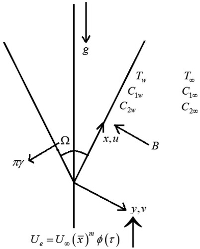
A 2-D laminar flow of an incompressible fluid (water) is considered in the direction of $x-$ axis and $y-$ axis is perpendicular to it. The $x$ and $y$ axis are used to measure the velocity components $u$ and $v$. An external magnetic field is applied in $y$-direction. The species components, liquid hydrogen and liquid oxygen diffusion, are considered, and equivalent realistic values of Schmidt numbers 160 and 340 at 27⁰C are considered [43]. The temperature variations between the fluid and the wall are thought to be quadratic in nature. The wall and ambient fluid temperature are taken to be $T_w$ and $T_{\mathrm{\infty }}$. Similarly, the concentration of liquid hydrogen $\left(C_1\right)$ and liquid oxygen $\left(C_2\right)$ at the wall, and away from the wall are considered to be $C_{1w},C_{2w}$ and $C_{1\mathrm{\infty }},C_{2\mathrm{\infty }}$, respectively. The wedge angle is taken as $\mathrm{\Omega }$ and the half-angle of the wedge $\left(\frac{\pi \gamma }{2}\right)$ as shown in Figure 1. Employing the Oberbeck-Boussinesq approximation for the buoyancy [44, 45], the physical properties of MHD, quadratic combined convection, and activation energy in the presence of time are represented by the following equations [30–32, 36]: (1) $\begin{array}{rl}& \frac{\mathrm{\partial }u}{\mathrm{\partial }x}+\frac{\mathrm{\partial }u}{\mathrm{\partial }y}=0,\end{array}$(1) (2) $\begin{array}{rl}& \frac{\mathrm{\partial }u}{\mathrm{\partial }t}+u\frac{\mathrm{\partial }u}{\mathrm{\partial }x}+v\frac{\mathrm{\partial }u}{\mathrm{\partial }y}\\ & =\frac{\mathrm{\partial }{U}_e}{\mathrm{\partial }t}+U_e\frac{\mathrm{\partial }{U}_e}{\mathrm{\partial }x}+\nu \left(\frac{{\mathrm{\partial }}^{2}u}{\mathrm{\partial }{y}^2}\right)-\frac{\sigma B^2}{\rho }\left(u-U_e\right)\\ & +g\left[{\text{β}}_1\right(T-T_{\mathrm{\infty }})+{\text{β}}_2{\left(T-T_{\mathrm{\infty }}\right)}^2+\cdots ]\\ & \times Cos\left(\frac{\pi \gamma }{2}\right)+g\left[{\text{β}}_3\right(C_1-C_{1\mathrm{\infty }})\\ & +{\text{β}}_4{\left(C_1-C_{1\mathrm{\infty }}\right)}^2+\cdots ]\\ & \times Cos\left(\frac{\pi \gamma }{2}\right)+g\left[{\text{β}}_5\right(C_2-C_{2\mathrm{\infty }})\\ & +{\text{β}}_6{\left(C_2-C_{2\mathrm{\infty }}\right)}^2+\cdots ]\times Cos\left(\frac{\pi \gamma }{2}\right),\end{array}$(2) (3) $\begin{array}{rl}& \frac{\mathrm{\partial }T}{\mathrm{\partial }t}+u\frac{\mathrm{\partial }T}{\mathrm{\partial }x}+v\frac{\mathrm{\partial }T}{\mathrm{\partial }y}=\frac{\nu }{Pr}\left(\frac{{\mathrm{\partial }}^{2}T}{\mathrm{\partial }{y}^2}\right)+\frac{\sigma B^2}{\rho C_p}(u-U_e{)}^2,\end{array}$(3) (4) $\begin{array}{rl}& \frac{\mathrm{\partial }{C}_1}{\mathrm{\partial }t}+u\frac{\mathrm{\partial }{C}_1}{\mathrm{\partial }x}+v\frac{\mathrm{\partial }{C}_1}{\mathrm{\partial }y}\\ & =\frac{\nu }{S{c}_1}\left(\frac{{\mathrm{\partial }}^2{C}_1}{\mathrm{\partial }{y}^2}\right)-K_{r_1}^2\left(C_1-C_{1\mathrm{\infty }}\right){\left(\frac{T}{T_{\mathrm{\infty }}}\right)}^{n_1}\\ & \times \mathrm{e}\mathrm{x}\mathrm{p}(-E_{a_1}/\kappa T),\end{array}$(4) (5) $\begin{array}{rl}& \frac{\mathrm{\partial }{C}_2}{\mathrm{\partial }t}+u\frac{\mathrm{\partial }{C}_2}{\mathrm{\partial }x}+v\frac{\mathrm{\partial }{C}_2}{\mathrm{\partial }y}\\ & =\frac{\nu }{S{c}_2}\left(\frac{{\mathrm{\partial }}^2{C}_2}{\mathrm{\partial }{y}^2}\right)-K_{r_2}^2\left(C_2-C_{2\mathrm{\infty }}\right){\left(\frac{T}{T_{\mathrm{\infty }}}\right)}^{n_2}\\ & \times \mathrm{e}\mathrm{x}\mathrm{p}(-E_{a_2}/\kappa T).\end{array}$(5) The initial conditions of the problem are: (6) $\begin{array}{r}u\left(x,y,0\right)=u_i\left(x,y\right);v\left(x,y,0\right)=v_i\left(x,y\right);\\ T\left(x,y,0\right)=T_i\left(x,y\right);C_1\left(x,y,0\right)={C_1}_i\left(x,y\right);\\ C_2\left(x,y,0\right)={C_2}_i\left(x,y\right).\end{array}$(6) The boundary constraints are: (7) $\begin{array}{l}\text{At}\eta =0:u\left(x,0,t\right)=0,v\left(x,0,t\right)=0,\\ T\left(x,0,t\right)=T_w,C_1\left(x,0,t\right)=C_{1w},\\ C_2\left(x,0,t\right)=C_{2w},\\ \text{As}\eta \to \mathrm{\infty }:u\left(x,\mathrm{\infty },t\right)\to U_e=U_e^{\ast }\varphi \left(\tau \right)\\ =U_{\mathrm{\infty }}(\overline{x}{)}^m\varphi \left(\tau \right),T\left(x,\mathrm{\infty },t\right)\to T_{\mathrm{\infty }},\\ C_1\left(x,\mathrm{\infty },t\right)\to C_{1\mathrm{\infty }},C_2\left(x,\mathrm{\infty },t\right)\to C_{2\mathrm{\infty }}.\end{array}\}$(7) Non-similar transformations: $\begin{array}{rl}\overline{x}& =\frac{x}{L};\eta ={\left[\frac{m+1}{2}\cdot \frac{U_e^{\ast }}{x\nu }\right]}^{1/2}y;\\ \tau & =\frac{m+1}{2L}{U}_{\mathrm{\infty }}\cdot (\overline{x}{)}^{m-1}t;\end{array}$ $\begin{array}{rl}m& =\frac{\overline{x}}{U_e^{\ast }}\cdot \frac{d{U}_e^{\ast }}{d\overline{x}}=\frac{\gamma }{2-\gamma };\end{array}$ $\begin{array}{rl}\psi \left(x,y,t\right)& ={\left[\frac{2}{m+1}x\nu U_e^{\ast }\right]}^{1/2}\varphi \left(\tau \right)f\left(\overline{x},\eta ,\tau \right);\text{where}\\ \varphi \left(\tau \right)& =1+\alpha {\tau }^2;\end{array}$ $\begin{array}{rl}u& =\frac{\mathrm{\partial }\psi }{\mathrm{\partial }y};v=-\frac{\mathrm{\partial }\psi }{\mathrm{\partial }x};\end{array}$ $\begin{array}{rl}G& =\frac{T-T_{\mathrm{\infty }}}{T_w-T_{\mathrm{\infty }}};H=\frac{C_1-C_{1\mathrm{\infty }}}{C_{1w}-C_{1\mathrm{\infty }}};\\ S& =\frac{C_2-C_{2\mathrm{\infty }}}{C_{2w}-C_{2\mathrm{\infty }}};\end{array}$ $\begin{array}{rl}u& =U_e^{\ast }\varphi F=U_{e}F;\end{array}$ $\begin{array}{rl}v& =-\left(\frac{2}{m+1}\frac{\nu U_e^{\ast }}{x}\right)\{\frac{m+1}{2}\varphi f+\overline{x}\varphi f_{\overline{x}}\\ & +\left(\frac{m-1}{2}\right)\varphi \eta F+\left(m-1\right)\varphi \tau f_{\tau }\\ & +\left(m-1\right)\tau {\varphi }_{\tau }f\phantom{\frac{m-1}{2}}\}.\end{array}$With the help of the above transformations, equation (1(1) $\begin{array}{rl}& \frac{\mathrm{\partial }u}{\mathrm{\partial }x}+\frac{\mathrm{\partial }u}{\mathrm{\partial }y}=0,\end{array}$(1) ) is satisfied trivially, and one can reduce eqs. (2)-(5) to nondimensional form in terms of $\overline{x},\eta ,\tau$ as follows: (8) $\begin{array}{rl}& F_{\eta \eta }+\varphi \left[f{F}_{\eta }+\frac{2m}{m+1}\left(1-F^2\right)\right]+{\varphi }^{-1}{\varphi }_{\tau }\left(1-F\right)-F_{\tau }\\ & -\frac{2\varphi \overline{x}}{m+1}\left(F{F}_{\overline{x}}-F_{\eta }{f}_{\overline{x}}\right)-2\left(\frac{m-1}{m+1}\right)\varphi \tau \left(F{F}_{\tau }-F_{\eta }{f}_{\tau }\right)\\ & -2\left(\frac{m-1}{m+1}\right)\tau {\varphi }_{\tau }\left[F^2-\left(f{F}_{\eta }+1\right)\right]\\ & -\frac{2}{m+1}Re{M}^2{N}_2\left(F-1\right)+\frac{2Ri{N}_1}{\varphi \left(m+1\right)}\left[G\right(1+{\text{β}}_{t}G)\\ & +N{c}_{1}H\left(1+{\text{β}}_{c_1}H\right)+N{c}_{2}S\left(1+{\text{β}}_{c_2}S\right)]=0,\end{array}$(8) (9) $\begin{array}{rl}& G_{\eta \eta }+Pr\varphi f{G}_{\eta }-Pr{G}_{\tau }-\frac{2Pr\varphi \overline{x}}{m+1}\left(F{G}_{\overline{x}}-G_{\eta }{f}_{\overline{x}}\right)\\ & -2Pr\left(\frac{m-1}{m+1}\right)\varphi \tau \left(F{G}_{\tau }-G_{\eta }{f}_{\tau }-{\varphi }^{-1}{\varphi }_{\tau }f{G}_{\eta }\right)\\ & +\frac{2}{m+1}PrEcRe{M}^2{N}_3{\varphi }^2(F-1{)}^2=0,\end{array}$(9) (10) $\begin{array}{rl}& H_{\eta \eta }+S{c}_1\varphi f{H}_{\eta }-S{c}_1{H}_{\tau }-\frac{2S{c}_1\varphi \overline{x}}{m+1}\left(F{H}_{\overline{x}}-H_{\eta }{f}_{\overline{x}}\right)\\ & -2S{c}_1\left(\frac{m-1}{m+1}\right)\varphi \tau \left(F{H}_{\tau }-H_{\eta }{f}_{\tau }-{\varphi }^{-1}{\varphi }_{\tau }f{H}_{\eta }\right)\\ & -\frac{2}{m+1}ReS{c}_1{K}_{c_1}{N}_{2}H(1+{\mathrm{\Omega }}_{T}G{)}^{n_1}{e}^{\left(-\frac{E_1}{\left(1+{\mathrm{\Omega }}_{T}G\right)}\right)}=0,\end{array}$(10) (11) $\begin{array}{rl}& S_{\eta \eta }+S{c}_2\varphi f{S}_{\eta }-S{c}_2{S}_{\tau }-\frac{2S{c}_2\varphi \overline{x}}{m+1}\left(F{S}_{\overline{x}}-S_{\eta }{f}_{\overline{x}}\right)\\ & -2S{c}_2\left(\frac{m-1}{m+1}\right)\varphi \tau \left(F{S}_{\tau }-S_{\eta }{f}_{\tau }-{\varphi }^{-1}{\varphi }_{\tau }f{S}_{\eta }\right)\\ & -\frac{2}{m+1}ReS{c}_2{K}_{c_2}{N}_{2}S(1+{\mathrm{\Omega }}_{T}G{)}^{n_2}{e}^{\left(-\frac{E_2}{\left(1+{\mathrm{\Omega }}_{T}G\right)}\right)}=0.\end{array}$(11) Equivalent boundary conditions: (12) $\begin{array}{rl}& \begin{array}{l}At\eta =0:F=0;G=1;H=1;S=1;\\ As\eta \to \mathrm{\infty }:F\to 1;G\to 0;H\to 0;S\to 0.\end{array}\}\end{array}$(12) $\begin{array}{rl}& \text{Where},Re=\frac{U_{\mathrm{\infty }}L}{\nu };M^2=\frac{\sigma B^2\nu }{\rho U_{\mathrm{\infty }}^2}\\ & Ri=\frac{g{\text{β}}_1\left(T_w-T_{\mathrm{\infty }}\right)L}{U_{\mathrm{\infty }}^2}Cos\left(\frac{\pi \gamma }{2}\right);\end{array}$ $\begin{array}{rl}& {\text{β}}_t=\frac{{\text{β}}_2}{{\text{β}}_1}\left(T_w-T_{\mathrm{\infty }}\right);N{c}_1=\frac{{\text{β}}_3\left(C_{1w}-C_{1\mathrm{\infty }}\right)}{{\text{β}}_1\left(T_w-T_{\mathrm{\infty }}\right)};\\ & {\text{β}}_{c_1}=\frac{{\text{β}}_4}{{\text{β}}_3}\left(C_{1w}-C_{1\mathrm{\infty }}\right);\end{array}$ $\begin{array}{rl}& N{c}_2=\frac{{\text{β}}_5\left(C_{2w}-C_{2\mathrm{\infty }}\right)}{{\text{β}}_1\left(T_w-T_{\mathrm{\infty }}\right)};{\text{β}}_{c_2}=\frac{{\text{β}}_6}{{\text{β}}_5}\left(C_{2w}-C_{2\mathrm{\infty }}\right);\\ & Ec=\frac{U_{\mathrm{\infty }}^2}{C_p\left(T_w-T_{\mathrm{\infty }}\right)};\end{array}$ $\begin{array}{rl}& Pr=\frac{\nu }{{\alpha }_m};S{c}_1=\frac{\nu }{D_{S_1}};S{c}_2=\frac{\nu }{D_{S_2}};\\ & {\mathrm{\Omega }}_T=\frac{\left(T_w-T_{\mathrm{\infty }}\right)}{T_{\mathrm{\infty }}};\end{array}$ $\begin{array}{rl}& N_1=\overline{x}\left(\frac{U_{\mathrm{\infty }}}{U_e^{\ast }}\right);N_2=\overline{x}{\left(\frac{U_{\mathrm{\infty }}}{U_e^{\ast }}\right)}^2;N_3=\overline{x}\left(\frac{U_e^{\ast }}{U_{\mathrm{\infty }}}\right);\\ & K{c}_1=\frac{K_{r_1}^2\nu }{U_{\mathrm{\infty }}^2};\end{array}$ $\begin{array}{rl}& K{c}_2=\frac{K_{r_2}^2\nu }{U_{\mathrm{\infty }}^2};E_1=-\frac{E_{a_1}}{\kappa T_{\mathrm{\infty }}};E_2=-\frac{E_{a_2}}{\kappa T_{\mathrm{\infty }}}.\end{array}$Let $\xi =(\overline{x}{)}^{\left(1-m\right)/2}$ be the dimensionless distance along the wedge $\left(\xi >0\right)$. Then, the nondimensional equations in terms of $\xi ,\eta ,\tau$ are: (13) $\begin{array}{rl}& F_{\eta \eta }+\varphi \left[f{F}_{\eta }+\frac{2m}{m+1}\left(1-F^2\right)\right]+{\varphi }^{-1}{\varphi }_{\tau }\left(1-F\right)-F_{\tau }\\ & -\frac{\left(1-m\right)}{m+1}\xi \varphi \left(F{F}_{\xi }-F_{\eta }{f}_{\xi }\right)-2\left(\frac{m-1}{m+1}\right)\varphi \tau \left(F{F}_{\tau }-F_{\eta }{f}_{\tau }\right)\\ & -2\left(\frac{m-1}{m+1}\right)\tau {\varphi }_{\tau }\left[F^2-\left(f{F}_{\eta }+1\right)\right]\\ & -\frac{2}{m+1}Re{M}^2{N}_5\left(F-1\right)+\frac{2Ri{N}_4}{\varphi \left(m+1\right)}\left[G\right(1+{\text{β}}_{t}G)\\ & +N{c}_{1}H\left(1+{\text{β}}_{c_1}H\right)+N{c}_{2}S\left(1+{\text{β}}_{c_2}S\right)]=0,\end{array}$(13) (14) $\begin{array}{rl}& G_{\eta \eta }+Pr\varphi f{G}_{\eta }-Pr{G}_{\tau }-\frac{\left(1-m\right)}{m+1}Pr\xi \varphi \left(F{G}_{\xi }-G_{\eta }{f}_{\xi }\right)\\ & -2Pr\left(\frac{m-1}{m+1}\right)\varphi \tau \left(F{G}_{\tau }-G_{\eta }{f}_{\tau }-{\varphi }^{-1}{\varphi }_{\tau }f{G}_{\eta }\right)\\ & +\frac{2}{m+1}PrEcRe{M}^2{N}_6{\varphi }^2(F-1{)}^2=0,\end{array}$(14) (15) $\begin{array}{rl}& H_{\eta \eta }+S{c}_1\varphi f{H}_{\eta }-S{c}_1{H}_{\tau }-\frac{\left(1-m\right)}{m+1}S{c}_1\varphi \xi \left(F{H}_{\xi }-H_{\eta }{f}_{\xi }\right)\\ & -2S{c}_1\left(\frac{m-1}{m+1}\right)\varphi \tau \left(F{H}_{\tau }-H_{\eta }{f}_{\tau }-{\varphi }^{-1}{\varphi }_{\tau }f{H}_{\eta }\right)\\ & -\frac{2}{m+1}ReS{c}_1{K}_{c_1}{N}_{5}H(1+{\mathrm{\Omega }}_{T}G{)}^{n_1}{e}^{\left(-\frac{E_1}{\left(1+{\mathrm{\Omega }}_{T}G\right)}\right)}=0,\end{array}$(15) (16) $\begin{array}{rl}& S_{\eta \eta }+S{c}_2\varphi f{S}_{\eta }-S{c}_2{S}_{\tau }-\frac{\left(1-m\right)}{m+1}S{c}_2\varphi \xi \left(F{S}_{\xi }-S_{\eta }{f}_{\xi }\right)\\ & -2S{c}_2\left(\frac{m-1}{m+1}\right)\varphi \tau \left(F{S}_{\tau }-S_{\eta }{f}_{\tau }-{\varphi }^{-1}{\varphi }_{\tau }f{S}_{\eta }\right)\\ & -\frac{2}{m+1}ReS{c}_2{K}_{c_2}{N}_{5}S(1+{\mathrm{\Omega }}_{T}G{)}^{n_2}{e}^{\left(-\frac{E_2}{\left(1+{\mathrm{\Omega }}_{T}G\right)}\right)}=0.\end{array}$(16) Pertinent boundary conditions are: (17) $\begin{array}{r}\begin{array}{l}At\eta =0:F=0;G=1;H=1;S=1;\\ As\eta \to \mathrm{\infty }:F\to 1;G\to 0;H\to 0;S\to 0.\end{array}\}\end{array}$(17) $\text{Where}{N}_4={\xi }^{\frac{2\left(1-2m\right)}{\left(1-m\right)}};N_5={\xi }^2;N_6={\xi }^{2\left(\frac{1+m}{1-m}\right)}.$Here $f\left(\xi ,\eta ,\tau \right)={\int }_0^{\eta }F\cdot d\eta +f_w$, where $f_w=0$ for the impervious surface.

Figure 1. Flow model.

The following engineering quantities give the constraints at the surface:

Surface drag coefficient: (18) $\begin{array}{rl}{C}_{fx}& =\frac{2\mu }{\rho {\left(U_e^{\ast }\right)}^2}{\left(\frac{\mathrm{\partial }u}{\mathrm{\partial }y}\right)}_{y=0}\\ & \Rightarrow R{e}_x^{1/2}{C}_{fx}=2\varphi {\left(\frac{m+1}{2}\right)}^{1/2}{F}_{\eta }\left(\xi ,0,\tau \right),\end{array}$(18) Energy transport strength: (19) $\begin{array}{l}N{u}_x=\frac{-x{\left(\frac{\mathrm{\partial }T}{\mathrm{\partial }y}\right)}_{y=0}}{\left(T_w-T_{\mathrm{\infty }}\right)}\\ \Rightarrow R{e}_x^{-1/2}N{u}_x=-{\left(\frac{m+1}{2}\right)}^{1/2}{G}_{\eta }\left(\xi ,0,\tau \right),\end{array}$(19) Mass transfer strength due to liquid hydrogen: (20) $\begin{array}{l}S{h}_{1x}=\frac{-x{\left(\frac{\mathrm{\partial }{C}_1}{\mathrm{\partial }y}\right)}_{y=0}}{\left(C_{1w}-C_{1\mathrm{\infty }}\right)}\\ \Rightarrow R{e}_x^{-1/2}S{h}_{1x}=-{\left(\frac{m+1}{2}\right)}^{1/2}{H}_{\eta }\left(\xi ,0,\tau \right),\end{array}$(20) Similarly, mass transfer strength due to liquid oxygen: (21) $\Rightarrow R{e}_x^{-1/2}S{h}_{2x}=-{\left(\frac{m+1}{2}\right)}^{1/2}{S}_{\eta }\left(\xi ,0,\tau \right).$(21)

2.1. Entropy generation

The following expression represents the entropy generation for the present modelled problem [4, 6,7, 11, 45–48]: $\begin{array}{rl}{S}_{gen}& =\underset{HeatTransferIrreversibility\left(HTI\right)}{\underbrace{\frac{k}{T^2}{\left(\frac{\mathrm{\partial }T}{\mathrm{\partial }y}\right)}^2}}+\underset{FluidFrictionIrreversibility\left(FFI\right)}{\underbrace{\frac{\mu }{T}{\left(\frac{\mathrm{\partial }u}{\mathrm{\partial }y}\right)}^2}}\\ & +\underset{EGduetoMagneticfield}{\underbrace{\frac{\sigma B^2}{T_{\mathrm{\infty }}}{\left(u-U_e\right)}^2}}\\ & +\underset{DiffusionIrreversibility\left(DI\right)}{\underbrace{\begin{array}{c}{\displaystyle \frac{R^{\ast }{D}_{S_1}}{C_{1\mathrm{\infty }}}}{\left({\displaystyle \frac{\mathrm{\partial }{C}_1}{\mathrm{\partial }y}}\right)}^2+{\displaystyle \frac{R^{\ast }{D}_{S_1}}{T_{\mathrm{\infty }}}}\left({\displaystyle \frac{\mathrm{\partial }{C}_1}{\mathrm{\partial }y}}{\displaystyle \frac{\mathrm{\partial }T}{\mathrm{\partial }y}}\right)\\ +{\displaystyle \frac{R^{\ast }{D}_{S_2}}{C_{2\mathrm{\infty }}}}{\left({\displaystyle \frac{\mathrm{\partial }{C}_2}{\mathrm{\partial }y}}\right)}^2+{\displaystyle \frac{R^{\ast }{D}_{S_2}}{T_{\mathrm{\infty }}}}\left({\displaystyle \frac{\mathrm{\partial }{C}_2}{\mathrm{\partial }y}}{\displaystyle \frac{\mathrm{\partial }T}{\mathrm{\partial }y}}\right)\\ +{\displaystyle \frac{R^{\ast }{D}_{S_{12}}}{C_{2\mathrm{\infty }}}}\left({\displaystyle \frac{\mathrm{\partial }{C}_1}{\mathrm{\partial }y}}{\displaystyle \frac{\mathrm{\partial }{C}_2}{\mathrm{\partial }y}}\right)\end{array}}}\end{array}$The first term HTI in the expression is that the EG results from heat transmission, whereas the second term FFI induces the EG by viscous dissipation or fluid friction. Next term is the EG due to the magnetic field. Further, EG induced by the diffusion of liquid oxygen and hydrogen is given by the fourth term DI. $S_{gen}$ is nondimensionalized $\left(S_G\right)$ by utilizing the characteristic entropy rate $S_0=\frac{\mathrm{\Delta }{T}^{2}k}{T_{\mathrm{\infty }}^2{x}^2}$. $\begin{array}{rl}\therefore S_G& =\frac{S_{gen}}{S_0}=P_1+P_2+P_3+P_4,\text{where}\\ P_1& =\frac{HTI}{S_0}=\frac{Re}{{\left(1+{\mathrm{\Omega }}_{T}G\right)}^2}\left(\frac{m+1}{2}\right)N_7{G}_{\eta }^2\end{array}$ $\begin{array}{rl}{P}_2& =\frac{FFI}{S_0}=\frac{ReBr{\varphi }^2}{{\mathrm{\Omega }}_T\left(1+{\mathrm{\Omega }}_{T}G\right)}\left(\frac{m+1}{2}\right)N_7^3{F}_{\eta }^2,\end{array}$ $\begin{array}{rl}{P}_3& =\frac{EGduetoMagneticfield}{S_0}\\ & =M^{2}ReBr{\varphi }^2{N}_7^2(F-1{)}^2,\end{array}$ $\begin{array}{rl}{P}_4& =\frac{DI}{S_0}=Re{N}_7\left(\frac{m+1}{2}\right)\\ & \times [M_1\frac{{\mathrm{\Omega }}_{c_1}}{{\mathrm{\Omega }}_T}{H}_{\eta }\left(\frac{{\mathrm{\Omega }}_{c_1}}{{\mathrm{\Omega }}_T}{H}_{\eta }+G_{\eta }\right)\\ & +M_2\frac{{\mathrm{\Omega }}_{c_2}}{{\mathrm{\Omega }}_T}{S}_{\eta }\left(\frac{{\mathrm{\Omega }}_{c_2}}{{\mathrm{\Omega }}_T}{S}_{\eta }+G_{\eta }\right)\end{array}$ $\begin{array}{rl}& +M_3\frac{{\mathrm{\Omega }}_{c_1}{\mathrm{\Omega }}_{c_2}}{{\mathrm{\Omega }}_T}{H}_{\eta }{S}_{\eta }].\end{array}$ $\begin{array}{rl}\text{Where},{\mathrm{\Omega }}_T& =\frac{\mathrm{\Delta }T}{T_{\mathrm{\infty }}},{\mathrm{\Omega }}_{c_1}=\frac{\mathrm{\Delta }{C}_1}{C_{1\mathrm{\infty }}},{\mathrm{\Omega }}_{c_2}=\frac{\mathrm{\Delta }{C}_2}{C_{2\mathrm{\infty }}},\\ M_1& =\frac{R^{\ast }{D}_{s_1}{C}_{1\mathrm{\infty }}}{k},M_2=\frac{R^{\ast }{D}_{s_2}{C}_{2\mathrm{\infty }}}{k},\\ M_3& =\frac{R^{\ast }{D}_{s_{12}}{C}_{1\mathrm{\infty }}}{k},Br=PrEc.\end{array}$

The expression for the Bejan number is given by: $Be=\frac{HTI}{S_G}=\frac{P_1}{P_1+P_2+P_3+P_4}.$

3. Numerical procedure

The following are the set of linear equations obtained by employing the Quasilineazation technique [36, 49–52] to the dimensionless eqs. (13)-(16). (22) $\begin{array}{rl}& F_{\eta \eta }^{i+1}+A_1^i{F}_{\eta }^{i+1}+A_2^i{F}_{\xi }^{i+1}+A_3^i{F}_{\tau }^{i+1}++A_4^i{F}^{i+1}\\ & +A_5^i{G}^{i+1}+A_6^i{H}^{i+1}+A_7^i{S}^{i+1}=A_8^i,\end{array}$(22) (23) $\begin{array}{rl}& G_{\eta \eta }^{i+1}+B_1^i{G}_{\eta }^{i+1}+B_2^i{G}_{\xi }^{i+1}+B_3^i{G}_{\tau }^{i+1}+B_4^i{F}^{i+1}=B_5^i,\end{array}$(23) (24) $\begin{array}{rl}& H_{\eta \eta }^{i+1}+C_1^i{H}_{\eta }^{i+1}+C_2^i{H}_{\xi }^{i+1}+C_3^i{H}_{\tau }^{i+1}+C_4^i{H}^{i+1}\\ & +C_5^i{F}^{i+1}+C_6^i{G}^{i+1}=C_7^i,\end{array}$(24) (25) $\begin{array}{rl}& S_{\eta \eta }^{i+1}+D_1^i{S}_{\eta }^{i+1}+D_2^i{S}_{\xi }^{i+1}+D_3^i{S}_{\tau }^{i+1}+D_4^i{S}^{i+1}\\ & +D_5^i{F}^{i+1}+D_6^i{G}^{i+1}=D_7^i.\end{array}$(25)

The equivalent boundary conditions are: (26) $\begin{array}{l}At\eta =0:F^{i+1}=0,G^{i+1}=1,\\ H^{i+1}=1,S^{i+1}=1,\\ As\eta ={\eta }_{\mathrm{\infty }}:F^{i+1}=1,G^{i+1}=0,\\ H^{i+1}=0,S^{i+1}=0.\end{array}\}$(26) The obtained set of linear equations (22)-(25) is subjected to the implicit finite difference technique [36, 53–56]. After that, Varga’s matrix inverse technique [57] is implemented to tackle the block tri-diagonal coefficient matrix. The answer is reached iteratively with a precision of 10⁻⁴. i. e., $\begin{array}{rl}& Max\{|(F_{\eta }{)}_w^{i+1}-(F_{\eta }{)}_w^i|,|(G_{\eta }{)}_w^{i+1}-(G_{\eta }{)}_w^i|,|(H_{\eta }{)}_w^{i+1}\\ & -(H_{\eta }{)}_w^i|,|(S_{\eta }{)}_w^{i+1}-(S_{\eta }{)}_w^i|\}\le {10}^{-4}\end{array}$The coefficients of equations (22)-(25) are: $\begin{array}{rl}{A}_1^i& =\varphi f+\left(\frac{m-1}{m+1}\right)\left[2\varphi \tau f_{\tau }+2\tau {\varphi }_{\tau }f-\varphi \xi f_{\xi }\right];\\ A_2^i& =-\left(\frac{1-m}{1+m}\right)\varphi \xi F;\\ A_3^i& =-\left[1+2\left(\frac{m-1}{m+1}\right)\varphi \tau F\right];\\ A_4^i& =-{\varphi }^{-1}{\varphi }_{\tau }-\frac{2}{m+1}\left(2m\varphi F+Re{M}^2{N}_5\right)\\ & -\left(\frac{m-1}{m+1}\right)\left(2\varphi \tau F_{\tau }+4\tau {\varphi }_{\tau }F-\varphi \xi F_{\xi }\right);\\ A_5^i& =\frac{2Ri{N}_4}{\varphi \left(m+1\right)}\left(1+2{\text{β}}_{t}G\right);\\ A_6^i& =\frac{2Ri{N}_4}{\varphi \left(m+1\right)}N{c}_1\left(1+2{\text{β}}_{c_1}H\right);\\ A_7^i& =\frac{2Ri{N}_4}{\varphi \left(m+1\right)}N{c}_2\left(1+2{\text{β}}_{c_2}S\right);\\ A_8^i& =-{\varphi }^{-1}{\varphi }_{\tau }-\frac{2}{m+1}\left[\phantom{\frac{Ri{N}_4}{\varphi }}\right(m+\left(m-1\right)\tau {\varphi }_{\tau }\left)\right(1+F^2)\\ & +Re{M}^2{N}_5+\left(\frac{1-m}{2}\right)\varphi \xi F{F}_{\xi }+\left(m-1\right)\varphi \tau F{F}_{\tau }\\ & -\frac{Ri{N}_4}{\varphi }\left({\text{β}}_t{G}^2+N{c}_1{\text{β}}_{c_1}{H}^2+N{c}_2{\text{β}}_{c_2}{S}^2\right)]\end{array}$ $\begin{array}{rl}{B}_1^i& =Pr\varphi \left[f+\left(\frac{m-1}{m+1}\right)\left(2\tau f_{\tau }+2\tau {\varphi }^{-1}{\varphi }_{\tau }f-\xi f_{\xi }\right)\right];\\ B_2^i& =-\left(\frac{1-m}{1+m}\right)Pr\varphi \xi F;\\ B_3^i& =-Pr\left[1+2\left(\frac{m-1}{m+1}\right)\varphi \tau F\right];\\ B_4^i& =-\frac{2}{m+1}Pr\varphi [\left(\frac{1-m}{2}\right)\xi G_{\xi }+(m-1)\tau G_{\tau }\\ & -2EcRe{M}^2\varphi N_6\left(F-1\right)\phantom{\frac{1-m}{2}}];\\ B_5^i& =\frac{2}{m+1}Pr\varphi \left[EcRe{M}^2\varphi N_6\right(F^2-1)-\left(\frac{1-m}{2}\right)\xi F{G}_{\xi }\\ & -\left(m-1\right)\tau F{G}_{\tau }];\end{array}$ $\begin{array}{rl}{C}_1^i& =S{c}_1\varphi \left[f+\left(\frac{m-1}{m+1}\right)\left(2\tau f_{\tau }+2\tau {\varphi }^{-1}{\varphi }_{\tau }f-\xi f_{\xi }\right)\right];\\ C_2^i& =-\left(\frac{1-m}{1+m}\right)S{c}_1\xi \varphi F;\\ C_3^i& =-S{c}_1\left[1+2\left(\frac{m-1}{m+1}\right)\varphi \tau F\right];\\ C_4^i& =-\left(\frac{2}{m+1}\right)ReS{c}_{1}K{c}_1{N}_5(1+{\mathrm{\Omega }}_{1}G{)}^{n_1}{e}^{-\left(\frac{E_1}{\left(1+{\mathrm{\Omega }}_{1}G\right)}\right)};\\ C_5^i& =-\left(\frac{m-1}{m+1}\right)S{c}_1\varphi \left[2\tau H_{\tau }-\xi H_{\xi }\right];\\ C_6^i& =\frac{C_4^{i}H}{\left(1+{\mathrm{\Omega }}_{1}G\right)}\left[\frac{E_1}{\left(1+{\mathrm{\Omega }}_{1}G\right)}+n_1{\mathrm{\Omega }}_1\right];\\ C_7^i& =C_5^{i}F+C_6^{i}G;\end{array}$ $\begin{array}{rl}{D}_1^i& =S{c}_2\varphi [f+\left(\frac{m-1}{m+1}\right)(2\tau f_{\tau }+2\tau {\varphi }^{-1}{\varphi }_{\tau }f-\xi f_{\xi }\left)\right];\\ D_2^i& =-\left(\frac{1-m}{1+m}\right)S{c}_2\xi \varphi F;\\ D_3^i& =-S{c}_2\left[1+2\left(\frac{m-1}{m+1}\right)\varphi \tau F\right];\\ D_4^i& =-\left(\frac{2}{m+1}\right)ReS{c}_{2}K{c}_2{N}_5(1+{\mathrm{\Omega }}_{1}G{)}^{n_2}{e}^{-\left(\frac{E_2}{\left(1+{\mathrm{\Omega }}_{1}G\right)}\right)};\\ D_5^i& =-\left(\frac{m-1}{m+1}\right)S{c}_2\varphi \left[2\tau S_{\tau }-\xi S_{\xi }\right];\\ D_6^i& =\frac{D_4^{i}S}{\left(1+{\mathrm{\Omega }}_{1}G\right)}\left[\frac{E_2}{\left(1+{\mathrm{\Omega }}_{1}G\right)}+n_2{\mathrm{\Omega }}_1\right];\\ D_7^i& =D_5^{i}F+D_6^{i}G.\end{array}$

3.1. Comparison of the current outcomes

The current steady-state findings of $F_{\eta }\left(\xi ,0\right)$ and $G_{\eta }\left(\xi ,0\right)$ are compared with those of Singh et al. [30] and Kumari et al. [31] in Table 1. The comparison reveals that the present outcomes are in good accord.

Table 1. A comparison of the current time-independent findings with [30] and [31] at $Pr=0.73$.

	Current findings		Singh et al. [30]		Kumari et al. [31]
Wedge angle parameter	$F_{\eta }\left(\xi ,0\right)$	$G_{\eta }\left(\xi ,0\right)$	$F_{\eta }\left(\xi ,0\right)$	$G_{\eta }\left(\xi ,0\right)$	$F_{\eta }\left(\xi ,0\right)$	$G_{\eta }\left(\xi ,0\right)$
0	0.46975	0.42061	0.46975	0.42046	0.46975	0.42079
0.0141	0.50475	0.42620	0.50481	0.42606	0.50472	0.42635
0.0435	0.56898	0.43567	0.56895	0.43559	0.56904	0.43597
0.0909	0.65495	0.44750	0.65490	0.44742	0.65501	0.44770
0.1429	0.73200	0.45718	0.73196	0.45705	0.73202	0.45728
0.2000	0.80212	0.46525	0.80208	0.46511	0.80214	0.46534
0.3333	0.92766	0.47822	0.92767	0.47815	0.92766	0.47840

4. Results and discussion

The parameter ranges taken into account to analyze the physical understanding and the flow behaviour of the results taken are as follows: $-1\le Ri\le 10$, $0\le {\text{β}}_t\le 1$, $-0.5\le \alpha \le 0.5$, $0.5\le \xi \le 0.75$, $0\le M\le 2$, $0\le E_1\le 2$, $0\le E_2\le 2$, $0.5\le K{c}_1\le 1.5$, $0.5\le K{c}_2\le 1.5$, $0.5\le {\mathrm{\Omega }}_T\le 2.0$, $0.0909\le m\le 0.2$ i.e. ${30}^0\le \mathrm{\Omega }\le {60}^0$ and the values of a few parameters are kept constant, such as, $Pr=7.0$ (water), $Ec=0.1$, ${\text{β}}_{c_1}={\text{β}}_{c_2}=N{c}_1=N{c}_2=0.1$, $n_1=n_2=0.2$, $\delta =0.1$, $Re=10$. Further, realistic values of the Schmidt number for liquid hydrogen $S{c}_1=160$ and liquid oxygen $S{c}_2=340$ at 27⁰ C [32] are considered.

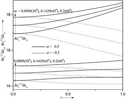
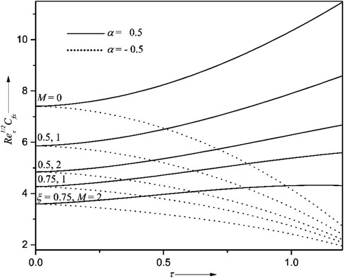
4.1. Variations of the wedge angle

The impact of wedge angle parameter $m$ and time $\tau$ on velocity profile $\left(F\left(\xi ,\eta ,\tau \right)\right)$, surface drag coefficient $\left(R{e}_x^{1/2}{C}_{fx}\right)$, and mass transfer rates of liquid hydrogen and oxygen $\left(R{e}_x^{-1/2}S{h}_{1x},R{e}_x^{-1/2}S{h}_{2x}\right)$ for accelerating $\left(\alpha >0\right)$, and decelerating flows $\left(\alpha <0\right)$ are deliberated in Figures 2–4. The wedge angle $\mathrm{\Omega }$ is directly proportional to $m$ i.e. when $m=0.0909$, $\mathrm{\Omega }={30}^0$ when $m=0.1429$, $\mathrm{\Omega }={45}^0$ and when $m=0.2$, $\mathrm{\Omega }={60}^0$. The increasing values of $m$ result in higher fluid velocity, surface drag coefficient and mass transfer rates for both $\tau =0$ and $\tau \ne 0$. Physically, by increasing the wedge angle, the fluid’s motion becomes more in the region near the wedge surface as the wedge becomes less slanted. Again, if the velocity is higher, the friction between the fluid particles and the wedge surface gradually improves and, consequently, the mass transfer rate. Also, it is inferred from Figures 2–4 that, as time surpasses, $F\left(\xi ,\eta ,\tau \right)$ diminishes and concurrently $R{e}_x^{1/2}{C}_{fx}$, $R{e}_x^{-1/2}S{h}_{1x},R{e}_x^{-1/2}S{h}_{2x}$ enhance for $\alpha >0$, reduce for $\alpha <0$. Particularly at $\tau =1$, $R{e}_x^{1/2}{C}_{fx}$, $R{e}_x^{-1/2}S{h}_{1x},R{e}_x^{-1/2}S{h}_{2x}$ surge approximately 11%, 10%, 7% respectively for $\alpha >0$ as the wedge angle becomes 60⁰ from 30⁰.

Figure 2. Impact of pressure gradient parameter $m$ and time $\tau$ on $F\left(\xi ,\eta ,\tau \right)$ for $\varphi \left(\tau \right)=1+\alpha {\tau }^2$ when $\alpha =0.5$, $\xi =0.5$, $Ri=10$, ${\text{β}}_t={\text{β}}_{c_1}={\text{β}}_{c_2}=0.1$, $N{c}_1=N{c}_2=0.1$, $M=Ec=0.1$, $n_1=n_2=0.2$, $K{c}_1=K{c}_2=E_1=E_2=\delta =0.1$, $Re=5$.

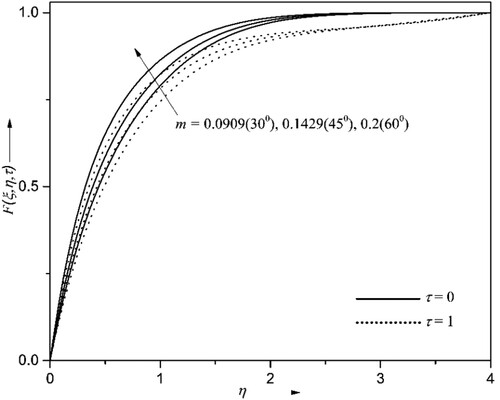
Figure 3. Impact of pressure gradient parameter $m$ and unsteadiness parameter $\alpha$ on $R{e}_x^{1/2}{C}_{fx}$ when $\xi =0.5$, $Ri=10$, ${\text{β}}_t={\text{β}}_{c_1}={\text{β}}_{c_2}=0.1$, $N{c}_1=N{c}_2=0.1$, $M=Ec=0.1$, $n_1=n_2=0.2$, $K{c}_1=K{c}_2=E_1=E_2=\delta =0.1$.

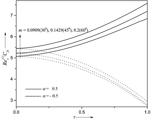
Figure 4. Impact of pressure gradient parameter $m$ and unsteadiness parameter $\alpha$ on $R{e}_x^{-1/2}S{h}_{1x},R{e}_x^{-1/2}S{h}_{2x}$ when $\xi =0.5$, $Ri=10$, ${\text{β}}_t={\text{β}}_{c_1}={\text{β}}_{c_2}=0.1$, $N{c}_1=N{c}_2=0.1$, $M=Ec=0.1$, $n_1=n_2=0.2$, $K{c}_1=K{c}_2=E_1=E_2=\delta =0.1$.

4.2. Magnetized field effect

Figures 5 and 6 explain the impact of the magnetic parameter $M$ along with the axial distance $\xi$ and time $\tau$ on the velocity profile $\left(F\left(\xi ,\eta ,\tau \right)\right)$ and the corresponding gradient $R{e}_x^{1/2}{C}_{fx}$. It is concluded from these figures that, $F\left(\xi ,\eta ,\tau \right)$ and $R{e}_x^{1/2}{C}_{fx}$ show the decaying nature for improving estimations of both $M$ and $\xi$. This is exemplified by the fact that enhancement in the values of $M$ induces a retarding force called the Lorentz force, which opposes the fluid’s motion and lessens the surface friction coefficient. Further, augmentation in $\xi$ functions as a negative pressure gradient in the momentum boundary layer. For instance, $R{e}_x^{1/2}{C}_{fx}$ diminishes approximately 64% whenever $M$ rises from 0 to 2 at $\tau =1$, $\xi =0.5$ for $\alpha >0$. The enrichment in the values of $\tau$ detracts $F\left(\xi ,\eta ,\tau \right)$ and propels the $R{e}_x^{1/2}{C}_{fx}$ for $\alpha >0$. The opposite nature is seen for $\alpha <0$ in case of $R{e}_x^{1/2}{C}_{fx}$.

Figure 5. Effect of magnetic parameter $M$, axial distance $\xi$ and time $\tau$ on $F\left(\xi ,\eta ,\tau \right)$ for $\varphi \left(\tau \right)=1+\alpha {\tau }^2$ when $\alpha =0.5$, $Ri=10$, ${\text{β}}_t={\text{β}}_{c_1}={\text{β}}_{c_2}=0.1$, $N{c}_1=N{c}_2=0.1$, $Ec=0.1$, $m=0.2$, $n_1=n_2=0.2$, $K{c}_1=K{c}_2=E_1=E_2=\delta =0.1$, $Re=5$.

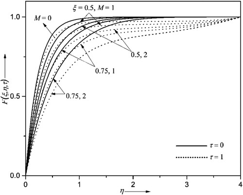
Figure 6. Effect of magnetic parameter $M$, axial distance $\xi$ and unsteadiness parameter $\alpha$ on $R{e}_x^{1/2}{C}_{fx}$ when $Ri=10$, ${\text{β}}_t={\text{β}}_{c_1}={\text{β}}_{c_2}=0.1$, $N{c}_1=N{c}_2=0.1$, $Ec=0.1$, $m=0.2$, $n_1=n_2=0.2$, $K{c}_1=K{c}_2=E_1=E_2=\delta =0.1$.

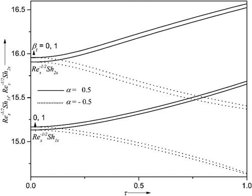
4.3. Quadratic combined convection effect on concentration profile and mass transfer rate

The variation of species concentration profiles $\left(H,S\right)\left(\xi ,\eta ,\tau \right)$ and the mass transfer rates $R{e}_x^{-1/2}S{h}_{1x},R{e}_x^{-1/2}S{h}_{2x}$ for distinct values of quadratic mixed convection parameter ${\text{β}}_t$ and time $\tau$ are outlined in Figures 7 and 8. It is known from the figures that the concentration profiles $\left(H,S\right)\left(\xi ,\eta ,\tau \right)$ weaken, and mass transfer rates intensify when mixed convection becomes nonlinear (quadratic) from linear one $\left(i.e.,{\text{β}}_{t}increasesfrom0to1\right)$. That is why the temperature disparity between the wedge surface and adjacent fluid becomes more significant. The species concentration profile lessens, and mass transfer boosts liquid oxygen diffusion $\left(S{c}_1=160\right)$ more than liquid hydrogen diffusion $\left(S{c}_2=340\right)$. For example, the mass transfer rate boosts up approximately by 9% for $S{c}_2=340$ in comparison with $S{c}_1=160$. Also, the boundary layer thickness is minimum for a higher Schmidt number $\left(Sc\right)$. Figure 8 elucidates that mass transfer rates $R{e}_x^{-1/2}S{h}_{1x},R{e}_x^{-1/2}S{h}_{2x}$ escalate for accelerating flow and lessen for decelerating flow.

Figure 7. Effect of quadratic combined convection parameter ${\text{β}}_t$ and time $\tau$ on $\left(H,S\right)\left(\xi ,\eta ,\tau \right)$ for $\varphi \left(\tau \right)=1+\alpha {\tau }^2$ when $\alpha =0.5$, $\xi =0.5$, $Ri=10$, ${\text{β}}_{c_1}={\text{β}}_{c_2}=0.1$, $N{c}_1=N{c}_2=0.1$, $M=Ec=0.1$, $m=0.2$, $n_1=n_2=0.2$, $K{c}_1=K{c}_2=E_1=E_2=\delta =0.1$, $Re=5$.

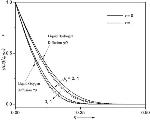
Figure 8. Effect of quadratic combined convection parameter ${\text{β}}_t$ and unsteadiness parameter $\alpha$ on $R{e}_x^{-1/2}S{h}_{1x},R{e}_x^{-1/2}S{h}_{2x}$ when $\xi =0.5$, $Ri=10$, ${\text{β}}_{c_1}={\text{β}}_{c_2}=0.1$, $N{c}_1=N{c}_2=0.1$, $M=Ec=0.1$, $m=0.2$, $n_1=n_2=0.2$, $K{c}_1=K{c}_2=E_1=E_2=\delta =0.1$.

4.4. Activation energy effects

Figures 9–12 display the influence of activation energies $E_1,E_2$ with chemical reaction parameters $K{c}_1,K{c}_2$ over liquid hydrogen $H\left(\xi ,\eta ,\tau \right)$ and liquid oxygen $S\left(\xi ,\eta ,\tau \right)$ concentration profiles and their corresponding mass transfers $R{e}_x^{-1/2}S{h}_{1x},R{e}_x^{-1/2}S{h}_{2x}$. The activation energy produces the least energy to the molecules or atoms to start a chemical reaction. This phenomenon allows us to investigate the supremacy of mass transportation using Arrhenius activation energy due to the binary chemical reaction. As seen by Figures 9 and 10, the activation energy boosts liquid hydrogen and oxygen concentration distributions, while Kc lowers the concentration distribution. Meanwhile, the opposite kind of nature can be seen in their mass transfer coefficients for the same values of activation energy and chemical reaction parameters. This behaviour is due to advanced values of the chemical reaction parameter leading to more destructive chemical reactions.

Figure 9. Influence of $K{c}_1$, activation energy $E_1$, and time $\tau$ on $H\left(\xi ,\eta ,\tau \right)$ for $\varphi \left(\tau \right)=1+\alpha {\tau }^2$ when $\alpha =0.5$, $\xi =0.5$, $Ri=10$, ${\text{β}}_t={\text{β}}_{c_1}={\text{β}}_{c_2}=0.1$, $N{c}_1=N{c}_2=0.1$, $M=Ec=0.1$, $m=0.2$, $n_1=n_2=0.2$, $K{c}_2=E_2=\delta =0.1$, $Re=5$.

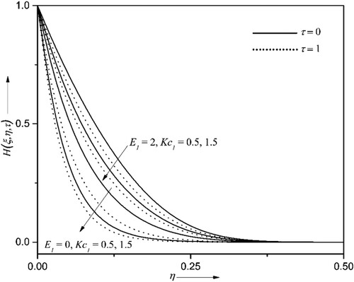
Figure 10. Influence of $K{c}_2$, activation energy $E_2$, and time $\tau$ on $S\left(\xi ,\eta ,\tau \right)$ for $\varphi \left(\tau \right)=1+\alpha {\tau }^2$ when $\alpha =0.5$, $\xi =0.5$, $Ri=10$, ${\text{β}}_t={\text{β}}_{c_1}={\text{β}}_{c_2}=0.1$, $N{c}_1=N{c}_2=0.1$, $M=Ec=0.1$, $m=0.2$, $n_1=n_2=0.2$, $K{c}_1=E_1=\delta =0.1$, $Re=5$.

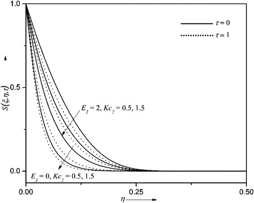
Figure 11. Influence of $K{c}_1$, activation energy $E_1$, and unsteadiness parameter $\alpha$ on $R{e}_x^{-1/2}S{h}_{1x}$ when $\xi =0.5$, $Ri=10$, ${\text{β}}_t={\text{β}}_{c_1}={\text{β}}_{c_2}=0.1$, $N{c}_1=N{c}_2=0.1$, $M=Ec=0.1$, $m=0.2$, $n_1=n_2=0.2$, $K{c}_2=E_2=\delta =0.1$.

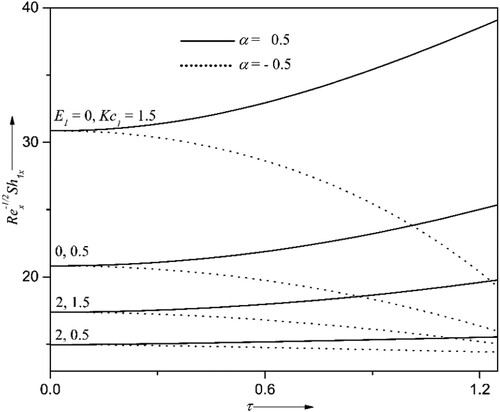
Figure 12. Influence of $K{c}_2$, activation energy $E_2$, and unsteadiness parameter $\alpha$ on $R{e}_x^{-1/2}S{h}_{2x}$ when $\xi =0.5$, $Ri=10$, ${\text{β}}_t={\text{β}}_{c_1}={\text{β}}_{c_2}=0.1$, $N{c}_1=N{c}_2=0.1$, $M=Ec=0.1$, $m=0.2$, $n_1=n_2=0.2$, $K{c}_2=E_2=\delta =0.1$.

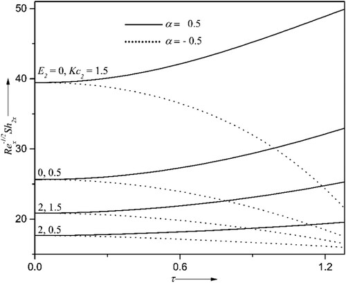
On the other hand, a low temperature and high activation energy result in a slower reaction rate. This results in higher species concentration and a lower mass transfer rate for higher activation energy. So, the mass transfer augments for enhanced values of chemical reaction parameters. In particular, when the chemical reaction parameter goes from 0.5–1.5, the mass transfer rates of liquid hydrogen and oxygen go up by about 23% and 25%, respectively, at $\tau =1$, $E_1=E_2=2$.

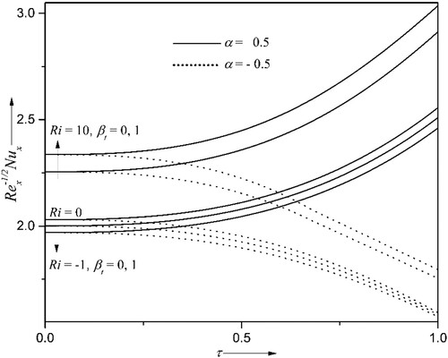
4.5. Effect of linear and nonlinear (quadratic) mixed convection

Figures 13 and 14 explore the combined effects of mixed $\left(Ri\right)$ and quadratic mixed convection $\left({\text{β}}_t\right)$ parameters over gradients of velocity and temperature, along with the time for accelerating and decelerating flows. The surface friction $\left(R{e}_x^{1/2}{C}_{fx}\right)$ and energy transfer rate $\left(R{e}_x^{-1/2}N{u}_x\right)$ are enhanced when mixed convection becomes nonlinear (quadratic) from linear $\left(i.e.,{\text{β}}_{t}increasesfrom0to1\right)$ in the case of aiding buoyancy flow $\left(Ri>0\right)$. The opposite trend is incurred in the case of opposing buoyancy flow $\left(Ri<0\right)$. Particularly, surface friction coefficient and energy transfer rate increased by approximately 15% and 10% when ${\text{β}}_t$ rises from 0 to 1 at $\tau =1$, respectively. It is because rising values of ${\text{β}}_t$ signifies the larger temperature difference between the wall and ambient fluid temperature. It is observed that mixed convection enhances $R{e}_x^{1/2}{C}_{fx}$, $R{e}_x^{-1/2}N{u}_x$ as it influences a positive pressure gradient. Further, the time has a commanding impact on these quantities. It improves the friction and energy transfer rate for accelerating flow $\left(\alpha >0\right)$ and the decelerating flow $\left(\alpha <0\right)$ lessens the friction and energy transfer rate.

Figure 13. Effect of $Ri$, ${\text{β}}_t$ and $\alpha$ on $R{e}_x^{1/2}{C}_{fx}$ when $Ri=10$, $\xi =0.5$, ${\text{β}}_{c_1}={\text{β}}_{c_2}=0.1$, $N{c}_1=N{c}_2=0.1$, $M=Ec=0.1$, $m=0.2$, $K{c}_1=K{c}_2=E_1=E_2=\delta =0.1$,$n_1=n_2=0.2$.

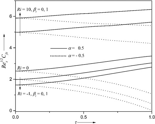
Figure 14. Effect of $Ri$, ${\text{β}}_t$ and $\alpha$ on $R{e}_x^{-1/2}N{u}_x$ when $Ri=10$, $\xi =0.5$, ${\text{β}}_{c_1}={\text{β}}_{c_2}=0.1$, $N{c}_1=N{c}_2=0.1$, $M=Ec=0.1$, $m=0.2$, $K{c}_1=K{c}_2=E_1=E_2=\delta =0.1$, $n_1=n_2=0.2$.

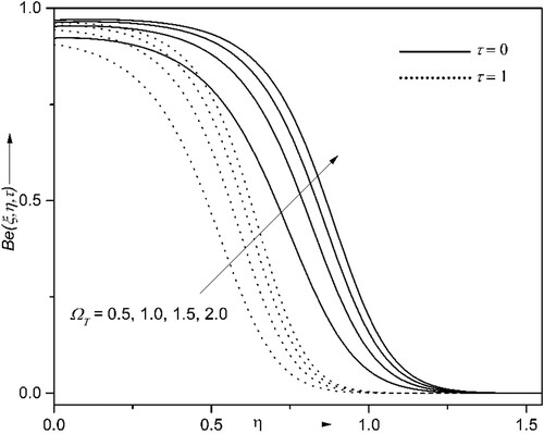
4.6. Consequences of entropy generation and Bejan number

The entropy generation (EG) $\left(S_G\right)$ and Bejan number $\left(Be\right)$ have been analyzed. The results are graphed in Figures 15–19 for the variations of Brinkman number $\left(Br\right)$, Reynolds’ number $\left(Re\right)$ and temperature difference ratio attribute $\left({\mathrm{\Omega }}_T\right)$. The higher values of $Br$ and $Re$ escalate the $S_G$ and consequently de-escalate the $Be$. The larger values of $Br$ indicate the slower conduction of heat produced due to viscous dissipation; hence fluid temperature becomes more and so does the EG. Also, the $S_G$ increases and $Be$ decreases as time surpass. It is noted from Figures 15, 17 and 18 that the fluctuations near the wall are due to the randomness in the system. Further, these fluctuations can be avoided by enhancing the magnitude of ${\mathrm{\Omega }}_T$ as seen in Figure 18. The EG can be minimized by upsurging the magnitude of ${\mathrm{\Omega }}_T$ as witnessed in Figure 18, and the $Be$ has the opposite nature, as it is inversely proportional to the EG. It can be concluded from the Figures 15–19 that the EG can be reduced by considering the larger magnitudes of ${\mathrm{\Omega }}_T$ and lower magnitudes of Re and Br.

Figure 15. Impact of $Br$ on $S_G$ for $\varphi \left(\tau \right)=1+\alpha {\tau }^2$, $\alpha =0.5$, when $Ri=10$, $\xi =0.5$, $S{c}_1=160$, $S{c}_2=340$, $Re=5$, ${\text{β}}_t={\text{β}}_{c_1}={\text{β}}_{c_1}=N{c}_1=N{c}_2=0.1$, $M_1=M_2=M_3=0.5$, and ${\mathrm{\Omega }}_T={\mathrm{\Omega }}_{c_1}={\mathrm{\Omega }}_{c_2}=0.5$.

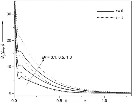
Figure 16. Impact of $Br$ on $Be$ for $\varphi \left(\tau \right)=1+\alpha {\tau }^2$, $\alpha =0.5$, when $Ri=10$, $\xi =0.5$, $S{c}_1=160$, $S{c}_2=340$, $Re=5$, ${\text{β}}_t={\text{β}}_{c_1}={\text{β}}_{c_1}=N{c}_1=N{c}_2=0.1$, $M_1=M_2=M_3=0.5$, and ${\mathrm{\Omega }}_T={\mathrm{\Omega }}_{c_1}={\mathrm{\Omega }}_{c_2}=0.5$.

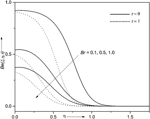
Figure 17. Impact of $Re$ on $S_G$ for $\varphi \left(\tau \right)=1+\alpha {\tau }^2$, $\alpha =0.5$, when $Ri=10$, $\xi =0.5$, $S{c}_1=160$, $S{c}_2=340$, $Br=0.1$, ${\text{β}}_t={\text{β}}_{c_1}={\text{β}}_{c_1}=N{c}_1=N{c}_2=0.1$, $M_1=M_2=M_3=0.5$, and ${\mathrm{\Omega }}_T={\mathrm{\Omega }}_{c_1}={\mathrm{\Omega }}_{c_2}=0.5$.

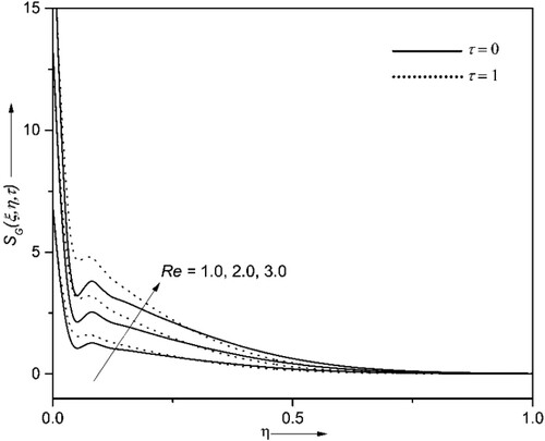
Figure 18. Impact of ${\mathrm{\Omega }}_T$ on $S_G$ for $\varphi \left(\tau \right)=1+\alpha {\tau }^2$, $\alpha =0.5$, when $Ri=10$, $\xi =0.5$, $S{c}_1=160$, $S{c}_2=340$, $Br=0.1$, ${\text{β}}_t={\text{β}}_{c_1}={\text{β}}_{c_1}=N{c}_1=N{c}_2=0.1$, $M_1=M_2=M_3=0.5$, ${\mathrm{\Omega }}_{c_1}={\mathrm{\Omega }}_{c_2}=0.5$, and $Re=5$.

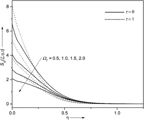
Figure 19. Impact of ${\mathrm{\Omega }}_T$ on $Be$ for $\varphi \left(\tau \right)=1+\alpha {\tau }^2$, $\alpha =0.5$, when $Ri=10$, $\xi =0.5$, $S{c}_1=160$, $S{c}_2=340$, $Br=0.1$, ${\text{β}}_t={\text{β}}_{c_1}={\text{β}}_{c_1}=N{c}_1=N{c}_2=0.1$, $M_1=M_2=M_3=0.5$, ${\mathrm{\Omega }}_{c_1}={\mathrm{\Omega }}_{c_2}=0.5$, and $Re=5$.

5. Conclusions

The influence of numerous emerging parameters on velocity, temperature, concentration profiles, and multiple gradients is described and graphically displayed. The discussions mentioned above resulted in the following findings:

• The mass transfer rates augment for enhanced values of chemical reaction parameters. In particular, when the chemical reaction parameter goes from 0.5–1.5, liquid hydrogen and oxygen mass transfer rates increase by about 23% and 25%, respectively, at $\tau =1$, $E_1=E_2=2$.

• Enhancing the wedge angle parameter $m$ upsurges the surface drag coefficient and mass transfer rates. Particularly at $\tau =1$, surface drag, mass transfer rates for liquid hydrogen and oxygen surge approximately 11%, 10%, 7%, respectively, for accelerating flow as the wedge angle becomes 60⁰ from 30⁰.

• It is noted that fluid velocity and surface friction show the decaying nature for improving estimations of both $M$ and $\xi$. For instance, the surface friction diminishes approximately 64% whenever $M$ rises from 0 to 2 at $\tau =1$, $\xi =0.5$ for $\alpha >0$.

• When mixed convection transitions from linear to nonlinear (quadratic) $\left(i.e.,{\text{β}}_{t}increasesfrom0to1\right)$, the surface friction and energy transfer ratestrengthen by about 15% and 10% when ${\text{β}}_t$ growths from 0 to 1 at $\tau =1$.

• The advanced values of $Br$ and $Re$ escalate the EG and consequently de-escalate the Bejan number. The larger values of $Br$ indicate the slower conduction of heat produced due to viscous dissipation; hence fluid temperature becomes more, and so does the EG.

• The fluctuations near the wall in $S_G$ are due to the randomness in the system. Further, these fluctuations can be avoided by enhancing the magnitude of ${\mathrm{\Omega }}_T$.

• The EG can be reduced by considering the larger magnitudes of ${\mathrm{\Omega }}_T$ and lower magnitudes of Re and Br.

Acknowledgement

The second author is thankful for the fellowship from the Department of Science and Technology-Innovation in Science Pursuit for Inspired Research (DST-INSPIRE), New Delhi.

Disclosure statement

No potential conflict of interest was reported by the author(s).

References

- Bestman AR. Natural convection boundary layer with suction and mass transfer in a porous medium. Int J Energy Res. 1990;14:389–396.
- Dhlamini M, Kameswaran PK, Sibanda P, et al. Activation energy and binary chemical reaction effects in mixed convective nanofluid flow with convective boundary conditions. J Comput Des Eng. 2019;6:149–158.
- Ali M, Shahzad M, Sultan F, et al. Exploring the features of stratification phenomena for 3D flow of Cross nanofluid considering activation energy. Int Commun Heat Mass Transf. 2020;116:104674.
- Alsaadi FE, Ullah I, Hayat T, et al. Entropy generation in nonlinear mixed convective flow of nanofluid in porous space influenced by Arrhenius activation energy and thermal radiation. J Therm Anal Calorim. 2020;140:799–809.
- RamReddy C, Naveen P. Analysis of activation energy in quadratic convective flow of a micropolar fluid with chemical reaction and suction/injection effects. Multidiscip Model Mater Struct. 2020;16:169–190.
- Khan MI, Alzahrani F. Numerical simulation for the mixed convective flow of non-Newtonian fluid with activation energy and entropy generation. Math Methods Appl Sci. 2021;44(9):7766–7777.
- Devi SSU, Mabood F. Entropy anatomization on Maran-goni Maxwell fluid over a rotating disk with nonlinear radiative flux and Arrhenius activation energy. Int Commun Heat Mass Transf. 2020;118:104857.
- Silverman M, Hallinan D. The relationship between self-diffusion activation energy and Soret coefficient in binary liquid mixtures. Chem Eng Sci. 2021;240:116660.
- Kumar A, Singh R, Sheremet MA. Analysis and modeling of magnetic dipole for the radiative flow of non-Newtonian nanomaterial with Arrhenius activation energy. Math Methods Appl Sci; https://doi.org/10.1002/mma.7124.
- Abbasi A, Gulzar S, Mabood F, et al. Nonlinear thermal radiation and activation energy features in axisymmetric rotational stagnation point flow of hybrid nanofluid. Int Commun Heat Mass Transf. 2021;126:105335.
- Khan ZH, Khan WA, Tang J, et al. Entropy generation analysis of triple diffusive flow past a horizontal plate in porous medium. Chem Eng Sci. 2020;228:115980.
- Ghalambaz M, Moattar F, Sheremet MA, et al. Triple-diffusive natural convection in a square porous cavity. Transp Porous Media. 2016;111(1):59–79.
- Khan WA, Culham JR, Khan ZH, et al. Triple diffusion along a horizontal plate in a porous medium with convective boundary condition. Int J Therm Sci. 2014;86:60–67.
- Patil PM, Shashikant A, Hiremath PS. Influence of liquid hydrogen and nitrogen on MHD triple diffusive mixed convection nanoliquid flow in presence of surface roughness. Int J Hydrog Energy. 2018;43:20101–20117.
- Sheikholeslami M, Said Z, Jafaryar M. Hydrothermal analysis for a parabolic solar unit with wavy absorber pipe and nanofluid. Renew Energy. 2022;188:922–932.
- Sheikholeslami M, Farshad SA. Nanoparticles transportation with turbulent regime through asolar collector with helical tapes. Adv Powder Technol. 2022;33(3):103510.
- Sheikholeslami M. Numerical investigation of solar system equipped with innovative turbulator and hybrid nanofluid. Sol Energy Mater Sol Cells. 2022;243:111786.
- Sheikholeslami M. Analyzing melting process of paraffin through the heat storage with honeycomb configuration utilizing nanoparticles. J Energy Storage. 2022;52(Part B):104954.
- Sheikholeslami M, Ebrahimpour Z. Nanofluid performance in a solar LFR system involving turbulator applying numerical simulation. Adv Powder Technol. 2022;33(8):103669.
- Noor A, Nazar R, Naganthran K, et al. Unsteady mixed convection flow at a three-dimensional stagnation point. Int J Numer Methods Heat Fluid Flow. 2021;31(1):236–250.
- Jenifer AS, Saikrishnan P, Lewis RW. Unsteady MHD mixed convection flow of water over a sphere with mass transfer. J Appl Comput Mech. 2021;7(2):935–943.
- Deniel YS, Aziz ZA, Ismail Z, et al. Double stratification effects on unsteady electrical MHD mixed convection flow of nanofluid with viscous dissipation and Joule heating. J Appl Res Technol. 2017;15:464–476.
- Patil PM, Pop I, Roy S. Unsteady heat and mass transfer over a vertical stretching sheet in a parallel free stream with variable wall temperature and concentration. Numer Methods Partial Differ Equ. 2012;28(3):926–941.
- Bejan A. A study of entropy generation in fundamental convective heat transfer. ASME J Heat Transf. 1979;101:718–725.
- Avellaneda JM, Bataille F, Toutant A, et al. Entropy generation minimization in a channel flow: Application to different advection-diffusion processes and boundary conditions. Chem Eng Sci. 2020;220:115601.
- Ardeh SS, Rafee R, Rashidi S. Heat transfer and entropy generation of hybrid nanofluid inside the convergent double-layer tapered microchannel. Math Methods Appl Sci; https://doi.org/10.1002/mma.8286.
- Sheikholeslami M, Ebrahimpour Z. Thermal improvement of linear Fresnel solar system utilizing Al2O3-water nanofluid and multi-way twisted tape. Int J Therm Sci. 2022;176:107505.
- Watanabe T, Funazaki K, Taniguchi H. Theoretical analysis on mixed convection boundary layer flow over a wedge with uniform suction or injection. Acta Mech. 1994;105:133–141.
- Kafoussias NG, Nanousis ND. Magnetohydrodynamic laminar boundary-layer flow over a wedge with suction or injection. Can J Phys. 1997;75:733–745.
- Singh PJ, Roy S, Ravindran R. Unsteady mixed convection flow over a vertical wedge. Int J Heat Mass Transf. 2009;52:415–421.
- Kumari M, Takhar HS, Nath G. Mixed convection flow over a vertical wedge embedded in a highly porous medium. Heat Mass Transf. 2001;37:139–146.
- Ganapathirao M, Ravindran R, Pop I. Non-uniform slot suction (injection) on an unsteady mixed convection flow over a wedge with chemical reaction and heat generation or absorption. Int J Heat Mass Transf. 2013;67:1054–1061.
- Patil PM, Kulkarni M, Tonannavar JR. A computational study of the triple-diffusive nonlinear convective nanoliquid flow over a wedge under convective boundary constraints. Int Commun Heat Mass Transf. 2021;128:105561.
- Nanousis ND. Theoretical magnetohydrodynamic analysis of mixed convection boundary-layer flow over a wedge with uniform suction or injection. Acta Mech. 1999;138:21–30.
- Ganapathirao M, Ravindran R, Momoniat E. Effects of chemical reaction, heat and mass transfer on an unsteady mixed convection boundary layer flow over a wedge with heat generation/absorption in the presence of suction or injection. Heat Mass Transf. 2015;51:289–300.
- Patil PM, Kulkarni M. A Numerical Study on MHD double diffusive nonlinear mixed convective nanofluid flow around a vertical wedge with diffusion of liquid hydrogen. J Egypt Math Soc. 2021;29(24).
- Bhattacharyya K, Pop I. MHD boundary layer flow due to an exponentially shrinking sheet. Magnetohydrodynamics. 2011;47:337–344.
- Shehzad N, Zeeshan A, Shakeel M, et al. Effects of Magnetohydrodynamics Flow on Multilayer Coatings of Newtonian and Non-Newtonian Fluids through Porous Inclined Rotating Channel. Coatings. 2022;12:430.
- Bhatti MM, Arain MB, Zeeshan A, et al. Swimming of Gyrotactic Microorganism in MHD Williamson nanofluid flow between rotating circular plates embedded in porous medium: Application of thermal energy storage. J Ene Storage. 2022;45:103511.
- Zeeshan A, Shehzad N, Abbas T, et al. Effects of Radiative Electro-Magnetohydrodynamics Diminishing Internal Energy of Pressure-Driven Flow of Titanium Dioxide-Water Nanofluid due to Entropy Generation. Entropy. 2019;21(3):236.
- Ishtiaq F, Ellahi R, Bhatti MM, et al. Insight in Thermally Radiative Cilia-Driven Flow of Electrically Conducting Non-Newtonian Jeffrey Fluid under the Influence of Induced Magnetic Field. Mathematics. 2022;10:2007.
- Mousa MM, Ali MR, Ma WX. A combined method for simulating MHD convection in square cavities through localized heating by method of line and penalty-artificial compressibility. J Taibah Univ Sci. 2021;15(1):208–217.
- Scribd. Mass diffusivity data, https://www.scribd.com/doc/58782633/MassDiffusivity-Data.
- Gray DD, Giorgini A. The validity of Boussinesq approximation for liquids and gases. Int J Heat Mass Transf. 1976;19:545–551.
- Schlichting H, Gersten K. Boundary layer theory. New York: Springer; 2000.
- Omri M, Bouterra M, Ouri H, et al. Entropy generation of nanofluid flow in hexagonal microchannel. J Taibah Univ Sci. 2022;16(1):75–88.
- Ellahi R, Alamri SZ, Basit A, et al. Effects of MHD and slip on heat transfer boundary layer flow over a moving plate based on specific entropy generation. J Taibah Univ Sci. 2018;12(4):476–482.
- Tlili I, Shamir N, Ramzan M, et al. A novel model to analyze Darcy Forchheimer nanofluid flow in a permeable medium with Entropy generation analysis. J Taibah Univ Sci. 2020;14(1):916–930.
- Patil PM, Roy M, Shashikant A, et al. Triple diffusive mixed convection from an exponentially decreasing mainstream velocity. Int J Heat Mass Transf. 2018;124:298–306.
- Patil PM, Doddagoudar SH, Hiremath PS. Impacts of surface roughness on mixed convection nanofluid flow with liquid hydrogen/nitrogen diffusion. Int J Num Methods Heat Fluid Flow. 2019;29(6):2146–2174.
- Radbill RJ, McCue AG. Quasilinearization and nonlinear problems in fluid and orbital mechanics. New York: Elsevier Publishing Co.; 1970.
- Bellman RE, Kalaba RE. Quasilinearization and nonlinear boundary value problems. New York: American Elsevier Publishing Co. Inc.; 1965.
- Inouye K, Tate A. Finite difference version of Quasilinearization applied to boundary layer equations. AIAA J. 1974;12:558–560.
- Patil PM, Kulkarni M, Hiremath PS. Effects of surface roughness on mixed convective nanofluid flow past an exponentially stretching permeable surface. Chin J Phys. 2020;64:203–218.
- Patil PM, Shankar HF, Hiremath PS, et al. Nonlinear mixed convective nanofluid flow about a rough sphere with the diffusion of liquid hydrogen. Alex Eng J. 2021;60(1):1043–1053.
- Patil PM, Kulkarni M. Nonlinear mixed convective nanofluid flow along moving vertical rough plate. Rev Mex de Fis. 2020;66(2):153–161.
- Varga RS. Matrix iterative analysis. USA: Prentice-Hall; 2000. 219-223.