A new study of soliton solutions for the variable coefficients Caudrey–Dodd–Gibbon equation

Abstract

We present a paper on the different methods for finding solutions to the Caudrey–Dodd–Gibbon equation with variable coefficients, which has wide applications in quantum mechanics and nonlinear optics. We have studied the equation analytically by using the unified method and the modified Kudryashov method. With the aid of symbolic computation and several types of auxiliary equations, we have obtained soliton solutions and other solutions. Then, we assign different values to the parameters, generating two-dimensional and three-dimensional graphics of the solutions, and discuss the interaction of several groups of solion solutions to form periodic wave solutions and kink solitary wave solutions.

Keywords:

• Soliton solutions
• the Caudrey–Dodd–Gibbon equation
• the unified method
• the modified Kudryashov method
• symbolic computation

1. Introduction

Nonlinear partial differential equations play a crucial role in the study of physical phenomena. Through symbolic calculation, we cannot only discover the properties of nonlinear partial differential equations [1–3], but also get the exact solutions about them. Therefore, solving partial differential equations is a significant research subject. With the rapid development of the scientific society, there have been some methods proposed to deal with the nonlinear partial differential equations. For example, a history approach [4], the fixed point technique [5], the new method [6], the modified $(G^{\prime }/G)$-expansion method [7,8], the novel generalized $(G^{\prime }/G)$ -expansion technique [9], the modified Kudryashov method [10–13], the extended simplest equation [14–16], the homotopy analysis transform method [17] and the united method [18] and so on.

In this paper, we will deal with the Caudrey–Dodd–Gibbon equation with variable coefficients (vcCDG) using the unified method and the modified Kudryashov method of the above methods. Up to now, Mickle methods are applied to Equation (1(1) $\begin{array}{rl}& u_t+{\sigma }_1(t)u_x{u}_{xx}+{\sigma }_2(t)u{u}_{xxx}+{\sigma }_3(t)u^2{u}_x\\ & +{\sigma }_4(t)u_{xxxxx}=0,\end{array}$(1) ) as yet, such as Hirota's bilinear method [19] is used to obtain some breather wave and lumps solutions to the CDG equation, the exp-function method [20] and the ($G^{\prime }/G$)-expansion method [21] find generalized solitary solutions and exact solutions respectively, the invariance properties, optimal system and group invariant solutions are investigated in [22], the approximate solutions are obtained by the variational iteration method [23], and the improved generalized Riccati equation mapping method [24] figures out exact solutions. Nevertheless, the unified method and the modified Kudryashov method have not been applied to the equation.

In fact, it has been shown that some known methods (the ($G^{\prime }/G$)-expansion method, the F-expansion method, the exp-function method and the rational expansion method and others) are special cases of the united method, which was established in 2012. The emergence of the unified method has solved a great many of equation problems, such as, the thermophoretic motion equation [25], the coupled Burgers equations [26], the Zakharov-Kuznetsov equation [27], the Benjamin–Bona–Mahony–Peregrine equation [28] and the generalized (2 + 1)-dimensional Boussinesq equation [29]. Moreover, the modified Kudryashov method is also an important method for solving partial differential equation problems, the generalized Schrödinger–Boussinesq equations [10], the Klein–Gordon equations [11], the Benjamin–Bona–Mahony–Peregrine equation [28] and the KdV–KZK equation [30] are all solved by the modified Kudryashov method.

Here, the vcCDG equation [31,32] reads, (1) $\begin{array}{rl}& u_t+{\sigma }_1(t)u_x{u}_{xx}+{\sigma }_2(t)u{u}_{xxx}+{\sigma }_3(t)u^2{u}_x\\ & +{\sigma }_4(t)u_{xxxxx}=0,\end{array}$(1) where $u=u(x,t)$, $u{u}_{xxx}$ and $u_{xxxxx}$ are dispersive terms, ${\sigma }_i(t)$ (i = 1, 2, 3, 4) are functions with t. As one of the fifth-order KdV, it can also describe the nonlinear phenomena in fluids or plasmas and is completely integrable [32]. Compared with existing articles, breather wave and lumps solutions, solitary solutions, exact solutions, group invariant solutions, and approximate solutions have been obtained [19–24]. Our primary mission is committed to using the unified method and the modified Kudryashov method to look for polynomial solutions, rational function solutions and travelling wave solutions so as to get more relevant properties of the equation. Some significant examples are given below.

When ${\sigma }_1(t)={\sigma }_2(t)=\alpha ,{\sigma }_3(t)=\frac{{\alpha }^2}{5},{\sigma }_4(t)=1$ [33], (2) $u_t+\alpha u_x{u}_{xx}+\alpha u{u}_{xxx}+\frac{{\alpha }^2}{5}{u}^2{u}_x+u_{xxxxx}=0,$(2) is completely integrable and has soliton solutions.

When ${\sigma }_1(t)={\sigma }_2(t)=30,{\sigma }_3(t)=180,{\sigma }_4(t)=1$ [34], (3) $u_t+30u_x{u}_{xx}+30u{u}_{xxx}+180u^2{u}_x+u_{xxxxx}=0,$(3) are used to model nonlinear dispersive waves such as laser optics and plasma physics.

The remaining sections of this paper are textured in what follows. In Section 2, we use the unified method to receive the solutions of Equation (1(1) $\begin{array}{rl}& u_t+{\sigma }_1(t)u_x{u}_{xx}+{\sigma }_2(t)u{u}_{xxx}+{\sigma }_3(t)u^2{u}_x\\ & +{\sigma }_4(t)u_{xxxxx}=0,\end{array}$(1) ) and draw graphs for analysis. In Section 3, we are devoted to the utilization of the modified Kudryashov method to the vcCDG equation. Finally, conclusions will be given in Section 4.

2. The unified method

In view of the operation steps of the method, the following hypothesis is framed: (4) $u=U({\xi }_1,{\xi }_2),{\xi }_1={\alpha }_{1}x+{\alpha }_{2}t,{\xi }_2={\beta }_{1}x+{\beta }_{2}t,$(4) where ${\alpha }_1$, ${\alpha }_2$, ${\beta }_1$ and ${\beta }_2$ are arbitrary constants. With the above travelling wave transformation, Equation (1(1) $\begin{array}{rl}& u_t+{\sigma }_1(t)u_x{u}_{xx}+{\sigma }_2(t)u{u}_{xxx}+{\sigma }_3(t)u^2{u}_x\\ & +{\sigma }_4(t)u_{xxxxx}=0,\end{array}$(1) ) becomes the following differential equation: (5) $\begin{array}{rl}& {\sigma }_1(t)(U_1{\alpha }_1+U_2{\beta }_1){\alpha }_1^2{U}_{11}+2{\sigma }_1(t)(U_1{\alpha }_1\\ & +U_2{\beta }_1){\alpha }_1{\beta }_1{U}_{12}+{\sigma }_1(t)(U_1{\alpha }_1+U_2{\beta }_1){\beta }_1^2{U}_{22}\\ & +{\sigma }_2(t)U{\alpha }_1^3{U}_{111}+3{\sigma }_2(t)U{\alpha }_1^2{\beta }_1{U}_{112}\\ & +3{\sigma }_2(t)U{\alpha }_1{\beta }_1^2{U}_{122}+3{\sigma }_2(t)U{\beta }_1^3{U}_{222}+{\alpha }_1^5{U}_{11111}\\ & {\sigma }_4(t)+5{\sigma }_4(t){\alpha }_1^4{\beta }_1{U}_{11112}+10{\sigma }_4(t){\alpha }_1^3{\beta }_1^2{U}_{11122}\\ & +10{\sigma }_4(t){\alpha }_1^2{\beta }_1^3{U}_{11222}+5{\sigma }_4(t){\alpha }_1{\beta }_1^4{U}_{12222}\\ & +U_1{\alpha }_2+U_2{\beta }_2+{\sigma }_3(t)(U_1{\alpha }_1+U_2{\beta }_1)U^2\\ & +{\sigma }_4(t){\beta }_1^5{U}_{22222}=0,\end{array}$(5) where $U_1=\frac{\text{d}U}{\text{d}{\xi }_1}$ and $U_2=\frac{\text{d}U}{\text{d}{\xi }_2}$.

For the given vcCDG equation with two independent variables ${\xi }_1$, ${\xi }_2$ and dependent variable U, the solutions of Equation (5(5) $\begin{array}{rl}& {\sigma }_1(t)(U_1{\alpha }_1+U_2{\beta }_1){\alpha }_1^2{U}_{11}+2{\sigma }_1(t)(U_1{\alpha }_1\\ & +U_2{\beta }_1){\alpha }_1{\beta }_1{U}_{12}+{\sigma }_1(t)(U_1{\alpha }_1+U_2{\beta }_1){\beta }_1^2{U}_{22}\\ & +{\sigma }_2(t)U{\alpha }_1^3{U}_{111}+3{\sigma }_2(t)U{\alpha }_1^2{\beta }_1{U}_{112}\\ & +3{\sigma }_2(t)U{\alpha }_1{\beta }_1^2{U}_{122}+3{\sigma }_2(t)U{\beta }_1^3{U}_{222}+{\alpha }_1^5{U}_{11111}\\ & {\sigma }_4(t)+5{\sigma }_4(t){\alpha }_1^4{\beta }_1{U}_{11112}+10{\sigma }_4(t){\alpha }_1^3{\beta }_1^2{U}_{11122}\\ & +10{\sigma }_4(t){\alpha }_1^2{\beta }_1^3{U}_{11222}+5{\sigma }_4(t){\alpha }_1{\beta }_1^4{U}_{12222}\\ & +U_1{\alpha }_2+U_2{\beta }_2+{\sigma }_3(t)(U_1{\alpha }_1+U_2{\beta }_1)U^2\\ & +{\sigma }_4(t){\beta }_1^5{U}_{22222}=0,\end{array}$(5) ) are written (6) $\begin{array}{rl}U({\xi }_1,{\xi }_2)& =p_0(t)+\sum _{i+j=1}^n{p}_{i,j}(t){\varphi }_1^i({\xi }_1){\varphi }_2^j({\xi }_2),\\ ({\varphi }_1^{\prime }({\xi }_1){)}^p& =\sum _{r=0}^{pk}{b}_r(t){\varphi }_1^r({\xi }_1),\\ ({\varphi }_2^{\prime }({\xi }_2){)}^p& =\sum _{r=0}^{pk}{c}_r(t){\varphi }_2^r({\xi }_2),p=1,2,\end{array}$(6) where $p_{i,j}(t)$, $b_r(t)$ and $c_r(t)$ are functions that contain t. Then, by balancing condition, we need to balance $U_{11111}$ and $U{U}_{111}$ in Equation (5(5) $\begin{array}{rl}& {\sigma }_1(t)(U_1{\alpha }_1+U_2{\beta }_1){\alpha }_1^2{U}_{11}+2{\sigma }_1(t)(U_1{\alpha }_1\\ & +U_2{\beta }_1){\alpha }_1{\beta }_1{U}_{12}+{\sigma }_1(t)(U_1{\alpha }_1+U_2{\beta }_1){\beta }_1^2{U}_{22}\\ & +{\sigma }_2(t)U{\alpha }_1^3{U}_{111}+3{\sigma }_2(t)U{\alpha }_1^2{\beta }_1{U}_{112}\\ & +3{\sigma }_2(t)U{\alpha }_1{\beta }_1^2{U}_{122}+3{\sigma }_2(t)U{\beta }_1^3{U}_{222}+{\alpha }_1^5{U}_{11111}\\ & {\sigma }_4(t)+5{\sigma }_4(t){\alpha }_1^4{\beta }_1{U}_{11112}+10{\sigma }_4(t){\alpha }_1^3{\beta }_1^2{U}_{11122}\\ & +10{\sigma }_4(t){\alpha }_1^2{\beta }_1^3{U}_{11222}+5{\sigma }_4(t){\alpha }_1{\beta }_1^4{U}_{12222}\\ & +U_1{\alpha }_2+U_2{\beta }_2+{\sigma }_3(t)(U_1{\alpha }_1+U_2{\beta }_1)U^2\\ & +{\sigma }_4(t){\beta }_1^5{U}_{22222}=0,\end{array}$(5) ), then we have $n=2(k-1)$, $k=2,3,\dots$.

Next, we will use the unified method to find the travelling wave solutions of Equation (5(5) $\begin{array}{rl}& {\sigma }_1(t)(U_1{\alpha }_1+U_2{\beta }_1){\alpha }_1^2{U}_{11}+2{\sigma }_1(t)(U_1{\alpha }_1\\ & +U_2{\beta }_1){\alpha }_1{\beta }_1{U}_{12}+{\sigma }_1(t)(U_1{\alpha }_1+U_2{\beta }_1){\beta }_1^2{U}_{22}\\ & +{\sigma }_2(t)U{\alpha }_1^3{U}_{111}+3{\sigma }_2(t)U{\alpha }_1^2{\beta }_1{U}_{112}\\ & +3{\sigma }_2(t)U{\alpha }_1{\beta }_1^2{U}_{122}+3{\sigma }_2(t)U{\beta }_1^3{U}_{222}+{\alpha }_1^5{U}_{11111}\\ & {\sigma }_4(t)+5{\sigma }_4(t){\alpha }_1^4{\beta }_1{U}_{11112}+10{\sigma }_4(t){\alpha }_1^3{\beta }_1^2{U}_{11122}\\ & +10{\sigma }_4(t){\alpha }_1^2{\beta }_1^3{U}_{11222}+5{\sigma }_4(t){\alpha }_1{\beta }_1^4{U}_{12222}\\ & +U_1{\alpha }_2+U_2{\beta }_2+{\sigma }_3(t)(U_1{\alpha }_1+U_2{\beta }_1)U^2\\ & +{\sigma }_4(t){\beta }_1^5{U}_{22222}=0,\end{array}$(5) ) in the case of $n=2$.

2.1. The solitary solutions

In this instance, the solutions of Equation (5(5) $\begin{array}{rl}& {\sigma }_1(t)(U_1{\alpha }_1+U_2{\beta }_1){\alpha }_1^2{U}_{11}+2{\sigma }_1(t)(U_1{\alpha }_1\\ & +U_2{\beta }_1){\alpha }_1{\beta }_1{U}_{12}+{\sigma }_1(t)(U_1{\alpha }_1+U_2{\beta }_1){\beta }_1^2{U}_{22}\\ & +{\sigma }_2(t)U{\alpha }_1^3{U}_{111}+3{\sigma }_2(t)U{\alpha }_1^2{\beta }_1{U}_{112}\\ & +3{\sigma }_2(t)U{\alpha }_1{\beta }_1^2{U}_{122}+3{\sigma }_2(t)U{\beta }_1^3{U}_{222}+{\alpha }_1^5{U}_{11111}\\ & {\sigma }_4(t)+5{\sigma }_4(t){\alpha }_1^4{\beta }_1{U}_{11112}+10{\sigma }_4(t){\alpha }_1^3{\beta }_1^2{U}_{11122}\\ & +10{\sigma }_4(t){\alpha }_1^2{\beta }_1^3{U}_{11222}+5{\sigma }_4(t){\alpha }_1{\beta }_1^4{U}_{12222}\\ & +U_1{\alpha }_2+U_2{\beta }_2+{\sigma }_3(t)(U_1{\alpha }_1+U_2{\beta }_1)U^2\\ & +{\sigma }_4(t){\beta }_1^5{U}_{22222}=0,\end{array}$(5) ) are (7) $\begin{array}{rl}U({\xi }_1,{\xi }_2)& =p_0(t)+p_{1,0}(t){\varphi }_1({\xi }_1)+p_{0,1}(t){\varphi }_2({\xi }_2)\\ & +p_{1,1}(t){\varphi }_1({\xi }_1){\varphi }_2({\xi }_2)+p_{2,0}(t){\varphi }_1^2({\xi }_1)\\ & +p_{0,2}(t){\varphi }_2^2({\xi }_2),\end{array}$(7) (8) $\begin{array}{rl}{\varphi }_1^{\prime }({\xi }_1)& =b_0(t)+b_1(t){\varphi }_1({\xi }_1)+b_2(t){\varphi }_1^2({\xi }_1),\\ {\varphi }_2^{\prime }({\xi }_2)& =c_0(t)+c_1(t){\varphi }_2({\xi }_2)+c_2(t){\varphi }_2^2({\xi }_2).\end{array}$(8) By taking Equations (7(7) $\begin{array}{rl}U({\xi }_1,{\xi }_2)& =p_0(t)+p_{1,0}(t){\varphi }_1({\xi }_1)+p_{0,1}(t){\varphi }_2({\xi }_2)\\ & +p_{1,1}(t){\varphi }_1({\xi }_1){\varphi }_2({\xi }_2)+p_{2,0}(t){\varphi }_1^2({\xi }_1)\\ & +p_{0,2}(t){\varphi }_2^2({\xi }_2),\end{array}$(7) ) and (8(8) $\begin{array}{rl}{\varphi }_1^{\prime }({\xi }_1)& =b_0(t)+b_1(t){\varphi }_1({\xi }_1)+b_2(t){\varphi }_1^2({\xi }_1),\\ {\varphi }_2^{\prime }({\xi }_2)& =c_0(t)+c_1(t){\varphi }_2({\xi }_2)+c_2(t){\varphi }_2^2({\xi }_2).\end{array}$(8) ) into Equation (5(5) $\begin{array}{rl}& {\sigma }_1(t)(U_1{\alpha }_1+U_2{\beta }_1){\alpha }_1^2{U}_{11}+2{\sigma }_1(t)(U_1{\alpha }_1\\ & +U_2{\beta }_1){\alpha }_1{\beta }_1{U}_{12}+{\sigma }_1(t)(U_1{\alpha }_1+U_2{\beta }_1){\beta }_1^2{U}_{22}\\ & +{\sigma }_2(t)U{\alpha }_1^3{U}_{111}+3{\sigma }_2(t)U{\alpha }_1^2{\beta }_1{U}_{112}\\ & +3{\sigma }_2(t)U{\alpha }_1{\beta }_1^2{U}_{122}+3{\sigma }_2(t)U{\beta }_1^3{U}_{222}+{\alpha }_1^5{U}_{11111}\\ & {\sigma }_4(t)+5{\sigma }_4(t){\alpha }_1^4{\beta }_1{U}_{11112}+10{\sigma }_4(t){\alpha }_1^3{\beta }_1^2{U}_{11122}\\ & +10{\sigma }_4(t){\alpha }_1^2{\beta }_1^3{U}_{11222}+5{\sigma }_4(t){\alpha }_1{\beta }_1^4{U}_{12222}\\ & +U_1{\alpha }_2+U_2{\beta }_2+{\sigma }_3(t)(U_1{\alpha }_1+U_2{\beta }_1)U^2\\ & +{\sigma }_4(t){\beta }_1^5{U}_{22222}=0,\end{array}$(5) ), we can set the coefficients of ${\varphi }_j({\xi }_j)$ to 0. Through symbolic computation, and making all the coefficients of ${\varphi }_j({\xi }_j)$($j=1,2$) equal to zero, we get (9) $\begin{array}{rl}& p_{1,1}(t)=0,{\sigma }_1(t)={\sigma }_2(t),p_{2,0}(t)={\displaystyle \frac{3{\alpha }_1{b}_2^2(t){\alpha }_2}{2R{\sigma }_2(t)}},\\ & p_{0,2}(t)={\displaystyle \frac{120{\beta }_1^2{c}_2^2(t){\alpha }_2}{80R{\sigma }_2(t){\alpha }_1}},\\ & p_{1,0}(t)={\displaystyle \frac{3{\alpha }_1{b}_2(t)b_1(t){\alpha }_2}{2R{\sigma }_2(t)}},\\ & p_{0,1}(t)={\displaystyle \frac{3{\beta }_1^2{c}_2(t)c_1(t){\alpha }_2}{2R{\sigma }_2(t){\alpha }_1}},\\ & {\sigma }_3(t)=-{\displaystyle \frac{4R{\sigma }_2^2(t){\alpha }_1}{{\alpha }_2}},\\ & p_0(t)={\displaystyle \frac{\begin{array}{c}{\alpha }_2(c_1^2(t){\beta }_1^2\\ +8{\beta }_1^2{c}_0(t)c_2(t)+8{\alpha }_1^2{b}_0(t)b_2(t)+{\alpha }_1^2{b}_1^2(t))\end{array}}{8R{\alpha }_1{\sigma }_2(t)}},\\ & {\sigma }_4(t)=-{\displaystyle \frac{{\alpha }_2}{20R{\alpha }_1}},\end{array}$(9) where $\begin{array}{rl}R& =-\frac{b_0^2(t)b_2^2(t){\alpha }_1^4}{5}+\frac{b_0(t)b_2(t)b_1^2(t){\alpha }_1^4}{10}-\frac{b_1^4(t){\alpha }_1^4}{80}\\ & +{(c_0(t)c_2(t)-\frac{c_1^2(t)}{4})}^2{\beta }_1^4.\end{array}$We can easily work out the solutions of Equation (8(8) $\begin{array}{rl}{\varphi }_1^{\prime }({\xi }_1)& =b_0(t)+b_1(t){\varphi }_1({\xi }_1)+b_2(t){\varphi }_1^2({\xi }_1),\\ {\varphi }_2^{\prime }({\xi }_2)& =c_0(t)+c_1(t){\varphi }_2({\xi }_2)+c_2(t){\varphi }_2^2({\xi }_2).\end{array}$(8) ) are (10) $\begin{array}{r}{\varphi }_1({\xi }_1)=-{\displaystyle \frac{\begin{array}{c}{b}_1(t)+(b_1^2(t)-4b_2(t)b_0(t))\tanh \\ (\frac{1}{2}(b_1^2(t)-4b_2(t)b_0(t)){\xi }_1)\end{array}}{2b_2(t)}},\\ {\varphi }_2({\xi }_2)=-{\displaystyle \frac{\begin{array}{c}{c}_1(t)+(c_1^2(t)-4c_2(t)c_0(t))\tanh \\ (\frac{1}{2}(c_1^2(t)-4c_2(t)c_0(t)){\xi }_2)\end{array}}{2c_2(t)}},\end{array}$(10) where $b_1^2(t)-4b_2(t)b_0(t)>0$ and $c_1^2(t)-4c_2(t)c_0(t)>0$. Then, by taking Equations (9(9) $\begin{array}{rl}& p_{1,1}(t)=0,{\sigma }_1(t)={\sigma }_2(t),p_{2,0}(t)={\displaystyle \frac{3{\alpha }_1{b}_2^2(t){\alpha }_2}{2R{\sigma }_2(t)}},\\ & p_{0,2}(t)={\displaystyle \frac{120{\beta }_1^2{c}_2^2(t){\alpha }_2}{80R{\sigma }_2(t){\alpha }_1}},\\ & p_{1,0}(t)={\displaystyle \frac{3{\alpha }_1{b}_2(t)b_1(t){\alpha }_2}{2R{\sigma }_2(t)}},\\ & p_{0,1}(t)={\displaystyle \frac{3{\beta }_1^2{c}_2(t)c_1(t){\alpha }_2}{2R{\sigma }_2(t){\alpha }_1}},\\ & {\sigma }_3(t)=-{\displaystyle \frac{4R{\sigma }_2^2(t){\alpha }_1}{{\alpha }_2}},\\ & p_0(t)={\displaystyle \frac{\begin{array}{c}{\alpha }_2(c_1^2(t){\beta }_1^2\\ +8{\beta }_1^2{c}_0(t)c_2(t)+8{\alpha }_1^2{b}_0(t)b_2(t)+{\alpha }_1^2{b}_1^2(t))\end{array}}{8R{\alpha }_1{\sigma }_2(t)}},\\ & {\sigma }_4(t)=-{\displaystyle \frac{{\alpha }_2}{20R{\alpha }_1}},\end{array}$(9) ) and (10(10) $\begin{array}{r}{\varphi }_1({\xi }_1)=-{\displaystyle \frac{\begin{array}{c}{b}_1(t)+(b_1^2(t)-4b_2(t)b_0(t))\tanh \\ (\frac{1}{2}(b_1^2(t)-4b_2(t)b_0(t)){\xi }_1)\end{array}}{2b_2(t)}},\\ {\varphi }_2({\xi }_2)=-{\displaystyle \frac{\begin{array}{c}{c}_1(t)+(c_1^2(t)-4c_2(t)c_0(t))\tanh \\ (\frac{1}{2}(c_1^2(t)-4c_2(t)c_0(t)){\xi }_2)\end{array}}{2c_2(t)}},\end{array}$(10) ) into Equations (7(7) $\begin{array}{rl}U({\xi }_1,{\xi }_2)& =p_0(t)+p_{1,0}(t){\varphi }_1({\xi }_1)+p_{0,1}(t){\varphi }_2({\xi }_2)\\ & +p_{1,1}(t){\varphi }_1({\xi }_1){\varphi }_2({\xi }_2)+p_{2,0}(t){\varphi }_1^2({\xi }_1)\\ & +p_{0,2}(t){\varphi }_2^2({\xi }_2),\end{array}$(7) ) and (8(8) $\begin{array}{rl}{\varphi }_1^{\prime }({\xi }_1)& =b_0(t)+b_1(t){\varphi }_1({\xi }_1)+b_2(t){\varphi }_1^2({\xi }_1),\\ {\varphi }_2^{\prime }({\xi }_2)& =c_0(t)+c_1(t){\varphi }_2({\xi }_2)+c_2(t){\varphi }_2^2({\xi }_2).\end{array}$(8) ), we can receive (11) $\begin{array}{rl}{u}_1(x,t)& ={\displaystyle \frac{-30{\alpha }_2}{\begin{array}{c}{\cosh }^2(-\frac{{\xi }_2{R}_1}{2})(\frac{b_1^4(t){\alpha }_1^4-5{\beta }_1^4{R}_1^2}{16}-\frac{b_1^2(t)b_0(t)b_2(t){\alpha }_1^4}{2}\\ +{\alpha }_1^4{b}_0^2(t)b_2^2(t)){\sigma }_2(t){\alpha }_1{\cosh }^2(2{\xi }_1{R}_2)\end{array}}}\\ & \times (((\frac{b_1^4(t){\alpha }_1^2}{16}-\frac{(b_0(t)b_2(t)+\frac{1}{12}){\alpha }_1^2{b}_1^2(t)}{2}\\ & +b_0^2(t)b_2^2(t){\alpha }_1^2+\frac{{\alpha }_1^2{b}_0(t)b_2(t)}{6}\\ & +\frac{R_1(R_1-\frac{2}{3}){\beta }_1^2}{16})\\ & \times {\cosh }^2(-\frac{{\xi }_2{R}_1}{2})-\frac{{\beta }_1^2{R}_1^2}{16}){\cosh }^2(2{\xi }_1{R}_2)\\ & -{\cosh }^2(-\frac{{\xi }_2{R}_1}{2}){\alpha }_1^2{R}_2^2\phantom{\frac{(b_0(t)b_2(t)+\frac{1}{12}){\alpha }_1^2{b}_1^2(t)}{2}}),\end{array}$(11) where ${\beta }_2=-\frac{\begin{array}{c}(-5b_0^2(t)b_2^2(t){\alpha }_1^4+\frac{5b_0(t)b_2(t)b_1^2(t){\alpha }_1^4}{2}-\frac{5b_1^4(t){\alpha }_1^4}{16}\\ +(c_0(t)c_2(t)-\frac{c_1^2(t)}{4}{)}^2{\beta }_1^4){\beta }_1{\alpha }_2\end{array}}{5R{\alpha }_1},$${\xi }_1={\alpha }_{1}x+{\alpha }_{2}t$, ${\xi }_2={\beta }_{1}x+{\beta }_{2}t$, $R_1=c_1^2(t)-4c_2(t)c_0(t)$ and $R_2=\frac{-b_1^2(t)}{4}+b_2(t)b_0(t)$.

Given the parameters of travelling wave solutions in Equation (11(11) $\begin{array}{rl}{u}_1(x,t)& ={\displaystyle \frac{-30{\alpha }_2}{\begin{array}{c}{\cosh }^2(-\frac{{\xi }_2{R}_1}{2})(\frac{b_1^4(t){\alpha }_1^4-5{\beta }_1^4{R}_1^2}{16}-\frac{b_1^2(t)b_0(t)b_2(t){\alpha }_1^4}{2}\\ +{\alpha }_1^4{b}_0^2(t)b_2^2(t)){\sigma }_2(t){\alpha }_1{\cosh }^2(2{\xi }_1{R}_2)\end{array}}}\\ & \times (((\frac{b_1^4(t){\alpha }_1^2}{16}-\frac{(b_0(t)b_2(t)+\frac{1}{12}){\alpha }_1^2{b}_1^2(t)}{2}\\ & +b_0^2(t)b_2^2(t){\alpha }_1^2+\frac{{\alpha }_1^2{b}_0(t)b_2(t)}{6}\\ & +\frac{R_1(R_1-\frac{2}{3}){\beta }_1^2}{16})\\ & \times {\cosh }^2(-\frac{{\xi }_2{R}_1}{2})-\frac{{\beta }_1^2{R}_1^2}{16}){\cosh }^2(2{\xi }_1{R}_2)\\ & -{\cosh }^2(-\frac{{\xi }_2{R}_1}{2}){\alpha }_1^2{R}_2^2\phantom{\frac{(b_0(t)b_2(t)+\frac{1}{12}){\alpha }_1^2{b}_1^2(t)}{2}}),\end{array}$(11) ), ${\alpha }_1=1$, ${\alpha }_2=1$, ${\beta }_1=-1$, ${\sigma }_2(t)=1$, $c_0(t)=-1$, $c_1(t)=\frac{1}{2}+\sin (t)$, $c_2(t)=1$, $b_0(t)=1$, $b_1(t)=1$ and $b_2(t)=-\frac{1}{2}$, 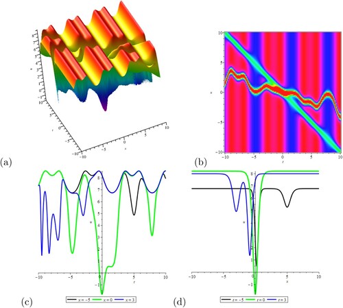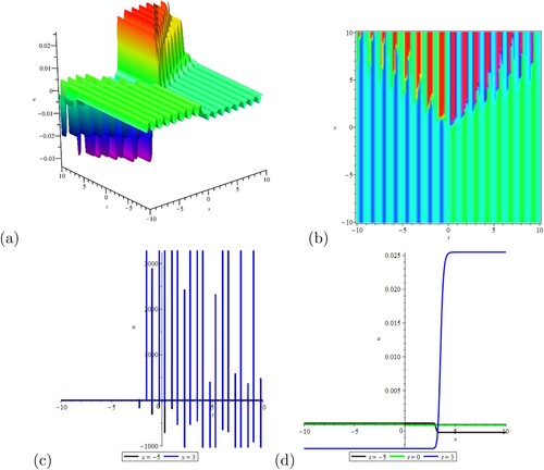we can obtain Figure 1. (a) and (b) illustrate the interaction between two-soliton waves with two different velocities. And they converge into one wave at the origin and gradually split into two waves, which travel in the other direction. Moreover, we can see that except $x=0$ and near the origin, the values of other solutions are all greater than zero in (c). Similarly, in (d), except $t=0$ and near the origin, the values of other solutions are all greater than zero.

Figure 1. The solitary wave solution obtained from Equation (7(7) $\begin{array}{rl}U({\xi }_1,{\xi }_2)& =p_0(t)+p_{1,0}(t){\varphi }_1({\xi }_1)+p_{0,1}(t){\varphi }_2({\xi }_2)\\ & +p_{1,1}(t){\varphi }_1({\xi }_1){\varphi }_2({\xi }_2)+p_{2,0}(t){\varphi }_1^2({\xi }_1)\\ & +p_{0,2}(t){\varphi }_2^2({\xi }_2),\end{array}$(7) ) with ${\alpha }_1=1$, ${\alpha }_2=1$, ${\beta }_1=-1$, ${\sigma }_2(t)=1$, $c_0(t)=-1$, $c_1(t)=\frac{1}{2}+\sin (t)$, $c_2(t)=1$, $b_0(t)=1$, $b_1(t)=1$ and $b_2(t)=-\frac{1}{2}$. (a) of 3D-plot; (b) of contour plot; (c) of u-t plot; (d) of u-x plot.

2.2. The soliton solutions

In order to solve Equation (5(5) $\begin{array}{rl}& {\sigma }_1(t)(U_1{\alpha }_1+U_2{\beta }_1){\alpha }_1^2{U}_{11}+2{\sigma }_1(t)(U_1{\alpha }_1\\ & +U_2{\beta }_1){\alpha }_1{\beta }_1{U}_{12}+{\sigma }_1(t)(U_1{\alpha }_1+U_2{\beta }_1){\beta }_1^2{U}_{22}\\ & +{\sigma }_2(t)U{\alpha }_1^3{U}_{111}+3{\sigma }_2(t)U{\alpha }_1^2{\beta }_1{U}_{112}\\ & +3{\sigma }_2(t)U{\alpha }_1{\beta }_1^2{U}_{122}+3{\sigma }_2(t)U{\beta }_1^3{U}_{222}+{\alpha }_1^5{U}_{11111}\\ & {\sigma }_4(t)+5{\sigma }_4(t){\alpha }_1^4{\beta }_1{U}_{11112}+10{\sigma }_4(t){\alpha }_1^3{\beta }_1^2{U}_{11122}\\ & +10{\sigma }_4(t){\alpha }_1^2{\beta }_1^3{U}_{11222}+5{\sigma }_4(t){\alpha }_1{\beta }_1^4{U}_{12222}\\ & +U_1{\alpha }_2+U_2{\beta }_2+{\sigma }_3(t)(U_1{\alpha }_1+U_2{\beta }_1)U^2\\ & +{\sigma }_4(t){\beta }_1^5{U}_{22222}=0,\end{array}$(5) ), the structure of solutions is hypothesized (12) $\begin{array}{rl}U({\xi }_1,{\xi }_2)& =p_0(t)+p_{1,0}(t){\varphi }_1({\xi }_1)+p_{0,1}(t){\varphi }_2({\xi }_2)\\ & +p_{1,1}(t){\varphi }_1({\xi }_1){\varphi }_2({\xi }_2)+p_{2,0}(t){\varphi }_1^2({\xi }_1)\\ & +p_{0,2}(t){\varphi }_2^2({\xi }_2),\end{array}$(12) (13) $\begin{array}{rl}& {\varphi }_1^{\prime }({\xi }_1)={\varphi }_1({\xi }_1)\sqrt{\begin{array}{c}{b}_0(t)+b_1(t){\varphi }_1({\xi }_1)\\ +b_2(t){\varphi }_1^2({\xi }_1)\end{array}},\\ & {\varphi }_2^{\prime }({\xi }_2)={\varphi }_2({\xi }_2)\sqrt{\begin{array}{c}{c}_0(t)+c_1(t){\varphi }_2({\xi }_2)\\ +c_2(t){\varphi }_2^2({\xi }_2)\end{array}}.\end{array}$(13) Substituting Equations (12(12) $\begin{array}{rl}U({\xi }_1,{\xi }_2)& =p_0(t)+p_{1,0}(t){\varphi }_1({\xi }_1)+p_{0,1}(t){\varphi }_2({\xi }_2)\\ & +p_{1,1}(t){\varphi }_1({\xi }_1){\varphi }_2({\xi }_2)+p_{2,0}(t){\varphi }_1^2({\xi }_1)\\ & +p_{0,2}(t){\varphi }_2^2({\xi }_2),\end{array}$(12) ) and (13(13) $\begin{array}{rl}& {\varphi }_1^{\prime }({\xi }_1)={\varphi }_1({\xi }_1)\sqrt{\begin{array}{c}{b}_0(t)+b_1(t){\varphi }_1({\xi }_1)\\ +b_2(t){\varphi }_1^2({\xi }_1)\end{array}},\\ & {\varphi }_2^{\prime }({\xi }_2)={\varphi }_2({\xi }_2)\sqrt{\begin{array}{c}{c}_0(t)+c_1(t){\varphi }_2({\xi }_2)\\ +c_2(t){\varphi }_2^2({\xi }_2)\end{array}}.\end{array}$(13) ) into Equation (5(5) $\begin{array}{rl}& {\sigma }_1(t)(U_1{\alpha }_1+U_2{\beta }_1){\alpha }_1^2{U}_{11}+2{\sigma }_1(t)(U_1{\alpha }_1\\ & +U_2{\beta }_1){\alpha }_1{\beta }_1{U}_{12}+{\sigma }_1(t)(U_1{\alpha }_1+U_2{\beta }_1){\beta }_1^2{U}_{22}\\ & +{\sigma }_2(t)U{\alpha }_1^3{U}_{111}+3{\sigma }_2(t)U{\alpha }_1^2{\beta }_1{U}_{112}\\ & +3{\sigma }_2(t)U{\alpha }_1{\beta }_1^2{U}_{122}+3{\sigma }_2(t)U{\beta }_1^3{U}_{222}+{\alpha }_1^5{U}_{11111}\\ & {\sigma }_4(t)+5{\sigma }_4(t){\alpha }_1^4{\beta }_1{U}_{11112}+10{\sigma }_4(t){\alpha }_1^3{\beta }_1^2{U}_{11122}\\ & +10{\sigma }_4(t){\alpha }_1^2{\beta }_1^3{U}_{11222}+5{\sigma }_4(t){\alpha }_1{\beta }_1^4{U}_{12222}\\ & +U_1{\alpha }_2+U_2{\beta }_2+{\sigma }_3(t)(U_1{\alpha }_1+U_2{\beta }_1)U^2\\ & +{\sigma }_4(t){\beta }_1^5{U}_{22222}=0,\end{array}$(5) ), and gathering the power of ${\varphi }_1({\xi }_1)$ and ${\varphi }_2({\xi }_2)$, we have the following results: (14) $\begin{array}{rl}& p_{1,1}(t)=0,{\sigma }_1(t)={\sigma }_2(t),\\ & p_{2,0}(t)=-{\displaystyle \frac{30{\alpha }_1^2{\beta }_2{b}_1^2(t)}{b_0(t){\sigma }_2(t){\beta }_{1}S}},\\ & c_2(t)={\displaystyle \frac{c_1^2(t)}{4c_0(t)}},\\ & p_{0,2}(t)=-{\displaystyle \frac{30{\beta }_1{\beta }_2{c}_1^2(t)}{c_0(t){\sigma }_2(t)S}},p_{1,0}(t)=-{\displaystyle \frac{60{\alpha }_1^2{\beta }_2{b}_1(t)}{{\sigma }_2(t){\beta }_{1}S}},\\ & p_{0,1}(t)=-{\displaystyle \frac{60{\beta }_1{\beta }_2{c}_1(t)}{{\sigma }_2(t)S}},\\ & {\sigma }_3(t)={\displaystyle \frac{{\sigma }_2^2(t){\beta }_{1}S}{20{\beta }_2}},b_2(t)={\displaystyle \frac{b_1^2(t)}{4b_0(t)}},\\ & p_0(t)=-{\displaystyle \frac{10{\beta }_2({\beta }_1^2{c}_0(t)+{\alpha }_1^2{b}_0(t))}{{\sigma }_2(t){\beta }_{1}S}},\\ & {\sigma }_4(t)={\displaystyle \frac{4{\beta }_2}{{\beta }_{1}S}},\end{array}$(14) where $S={\beta }_1^4{c}_0^2(t)-5{\alpha }_1^4{b}_0^2(t)$.

The solutions of auxiliary equations ${\varphi }_1({\xi }_1)$ and ${\varphi }_2({\xi }_2)$ in Equation (13(13) $\begin{array}{rl}& {\varphi }_1^{\prime }({\xi }_1)={\varphi }_1({\xi }_1)\sqrt{\begin{array}{c}{b}_0(t)+b_1(t){\varphi }_1({\xi }_1)\\ +b_2(t){\varphi }_1^2({\xi }_1)\end{array}},\\ & {\varphi }_2^{\prime }({\xi }_2)={\varphi }_2({\xi }_2)\sqrt{\begin{array}{c}{c}_0(t)+c_1(t){\varphi }_2({\xi }_2)\\ +c_2(t){\varphi }_2^2({\xi }_2)\end{array}}.\end{array}$(13) ) are (15) $\begin{array}{r}{\varphi }_1({\xi }_1)={\displaystyle \frac{-b_0(t)b_1(t)(\mathrm{sech}(\frac{\sqrt{b_0(t)}}{2}{\xi }_1){)}^2}{b_1^2(t)-b_0(t)b_2(t)(1-\tanh (\frac{\sqrt{b_0(t)}}{2}{\xi }_1){)}^2}},\\ {\varphi }_2({\xi }_2)={\displaystyle \frac{-c_0(t)c_1(t)(\mathrm{sech}(\frac{\sqrt{c_0(t)}}{2}{\xi }_2){)}^2}{c_1^2(t)-c_0(t)c_2(t)(1-\tanh (\frac{\sqrt{c_0(t)}}{2}{\xi }_2){)}^2}},\end{array}$(15) where $b_0(t)>0$ and $c_0(t)>0$. Advancing, as usual, we are able to have the solution of Equation (1(1) $\begin{array}{rl}& u_t+{\sigma }_1(t)u_x{u}_{xx}+{\sigma }_2(t)u{u}_{xxx}+{\sigma }_3(t)u^2{u}_x\\ & +{\sigma }_4(t)u_{xxxxx}=0,\end{array}$(1) ), (16) $\begin{array}{rl}{u}_2(x,t)& ={\displaystyle \frac{640{\alpha }_2}{\begin{array}{c}(8S_3^4+8S_3^3{S}_4+S_4{S}_3+1)\\ (8S_1^4+8S_1^3{S}_2+4S_2{S}_1+1){\alpha }_1\\ (5c_0^2(t){\beta }_1^4-b_0^2(t){\alpha }_1^4){\sigma }_2(t)\end{array}}}\\ & \times (((\phantom{\frac{25{\beta }_1^2{c}_0(t)+{\alpha }_1^2{b}_0(t)}{8}}{\beta }_1^2{c}_0(t)+{\alpha }_1^2{b}_0(t))S_1^4\\ & +({\beta }_1^2{c}_0(t){\alpha }_1^2{b}_0(t))S_1^3{S}_2\\ & -\frac{(11{\beta }_1^2{c}_0(t)-{\alpha }_1^2{b}_0(t))S_2{S}_1}{2}\\ & -6c_0(t)S_1^2{\beta }_1^2+\frac{25{\beta }_1^2{c}_0(t)+{\alpha }_1^2{b}_0(t)}{8})S_3^4\\ & +S_4(\phantom{\frac{25{\beta }_1^2{c}_0(t)+{\alpha }_1^2{b}_0(t)}{8}}({\beta }_1^2{c}_0(t)+{\alpha }_1^2{b}_0(t))S_1^4-6c_0(t)S_1^2{\beta }_1^2{S}_1^3\\ & \times ({\beta }_1^2{c}_0(t)+{\alpha }_1^2{b}_0(t))S_2\\ & -\frac{(11{\beta }_1^2{c}_0(t)-{\alpha }_1^2{b}_0(t))S_2{S}_1}{2}\\ & +\frac{25{\beta }_1^2{c}_0(t)+{\alpha }_1^2{b}_0(t)}{8})S_3^3-6S_3^2\\ & \times (S_1^4+S_1^3{S}_2+\frac{1}{2}{S}_2{S}_1+\frac{1}{8})b_0(t){\alpha }_1^2\\ & +\frac{1}{2}(\phantom{\frac{25{\beta }_1^2{c}_0(t)+{\alpha }_1^2{b}_0(t)}{8}}{S}_4(\phantom{\frac{25{\beta }_1^2{c}_0(t)+{\alpha }_1^2{b}_0(t)}{8}}({\beta }_1^2{c}_0(t)-11{\alpha }_1^2{b}_0(t))S_1^4\\ & -6c_0(t)S_1^2{\beta }_1^2+S_2{S}_1^3({\beta }_1^2{c}_0(t)\\ & -11{\alpha }_1^2{b}_0(t))-\frac{11({\beta }_1^2{c}_0(t)+{\alpha }_1^2{b}_0(t))S_2{S}_1}{2}\\ & +\frac{25{\beta }_1^2{c}_0(t)-11{\alpha }_1^2{b}_0(t)}{8})S_3)\\ & +\left(\frac{{\beta }_1^2{c}_0(t)+25{\alpha }_1^2{b}_0(t)}{8}\right)S_1^4\\ & +\left(\frac{{\beta }_1^2{c}_0(t)+25{\alpha }_1^2{b}_0(t)}{8}\right)S_1^3{S}_2\\ & -\frac{3c_0(t){\beta }_1^2{S}_1^2}{4}\\ & -\frac{(11{\beta }_1^2{c}_0(t)-25{\alpha }_1^2{b}_0(t))S_2{S}_1}{16}\\ & +\frac{25{\beta }_1^2{c}_0(t)+25{\alpha }_1^2{b}_0(t)}{64}),\end{array}$(16) where ${\xi }_1={\alpha }_{1}x+{\alpha }_{2}t$, ${\xi }_2={\beta }_{1}x+{\beta }_{2}t$, ${\alpha }_2=-\frac{{\alpha }_1{\beta }_2(5{\beta }_1^4{c}_0^2(t)-{\alpha }_1^4{b}_0^2(t))}{{\beta }_{1}S}$, $S_1=\cosh (\frac{{\xi }_2\sqrt{c_0(t)}}{2})$, $S_2=\sinh (\frac{{\xi }_2\sqrt{c_0(t)}}{2})$, $S_3=\cosh (\frac{{\xi }_1\sqrt{b_0(t)}}{2})$ and $S_4=\sinh (\frac{{\xi }_1\sqrt{b_0(t)}}{2})$.

We assign values to the free variables in Equation (16(16) $\begin{array}{rl}{u}_2(x,t)& ={\displaystyle \frac{640{\alpha }_2}{\begin{array}{c}(8S_3^4+8S_3^3{S}_4+S_4{S}_3+1)\\ (8S_1^4+8S_1^3{S}_2+4S_2{S}_1+1){\alpha }_1\\ (5c_0^2(t){\beta }_1^4-b_0^2(t){\alpha }_1^4){\sigma }_2(t)\end{array}}}\\ & \times (((\phantom{\frac{25{\beta }_1^2{c}_0(t)+{\alpha }_1^2{b}_0(t)}{8}}{\beta }_1^2{c}_0(t)+{\alpha }_1^2{b}_0(t))S_1^4\\ & +({\beta }_1^2{c}_0(t){\alpha }_1^2{b}_0(t))S_1^3{S}_2\\ & -\frac{(11{\beta }_1^2{c}_0(t)-{\alpha }_1^2{b}_0(t))S_2{S}_1}{2}\\ & -6c_0(t)S_1^2{\beta }_1^2+\frac{25{\beta }_1^2{c}_0(t)+{\alpha }_1^2{b}_0(t)}{8})S_3^4\\ & +S_4(\phantom{\frac{25{\beta }_1^2{c}_0(t)+{\alpha }_1^2{b}_0(t)}{8}}({\beta }_1^2{c}_0(t)+{\alpha }_1^2{b}_0(t))S_1^4-6c_0(t)S_1^2{\beta }_1^2{S}_1^3\\ & \times ({\beta }_1^2{c}_0(t)+{\alpha }_1^2{b}_0(t))S_2\\ & -\frac{(11{\beta }_1^2{c}_0(t)-{\alpha }_1^2{b}_0(t))S_2{S}_1}{2}\\ & +\frac{25{\beta }_1^2{c}_0(t)+{\alpha }_1^2{b}_0(t)}{8})S_3^3-6S_3^2\\ & \times (S_1^4+S_1^3{S}_2+\frac{1}{2}{S}_2{S}_1+\frac{1}{8})b_0(t){\alpha }_1^2\\ & +\frac{1}{2}(\phantom{\frac{25{\beta }_1^2{c}_0(t)+{\alpha }_1^2{b}_0(t)}{8}}{S}_4(\phantom{\frac{25{\beta }_1^2{c}_0(t)+{\alpha }_1^2{b}_0(t)}{8}}({\beta }_1^2{c}_0(t)-11{\alpha }_1^2{b}_0(t))S_1^4\\ & -6c_0(t)S_1^2{\beta }_1^2+S_2{S}_1^3({\beta }_1^2{c}_0(t)\\ & -11{\alpha }_1^2{b}_0(t))-\frac{11({\beta }_1^2{c}_0(t)+{\alpha }_1^2{b}_0(t))S_2{S}_1}{2}\\ & +\frac{25{\beta }_1^2{c}_0(t)-11{\alpha }_1^2{b}_0(t)}{8})S_3)\\ & +\left(\frac{{\beta }_1^2{c}_0(t)+25{\alpha }_1^2{b}_0(t)}{8}\right)S_1^4\\ & +\left(\frac{{\beta }_1^2{c}_0(t)+25{\alpha }_1^2{b}_0(t)}{8}\right)S_1^3{S}_2\\ & -\frac{3c_0(t){\beta }_1^2{S}_1^2}{4}\\ & -\frac{(11{\beta }_1^2{c}_0(t)-25{\alpha }_1^2{b}_0(t))S_2{S}_1}{16}\\ & +\frac{25{\beta }_1^2{c}_0(t)+25{\alpha }_1^2{b}_0(t)}{64}),\end{array}$(16) ), ${\alpha }_1=1$, ${\beta }_1=-1$, ${\beta }_2=-1$, ${\sigma }_2(t)=1+2\cos (2t)$, $b_0(t)=-1$ and $c_0(t)=-1$, 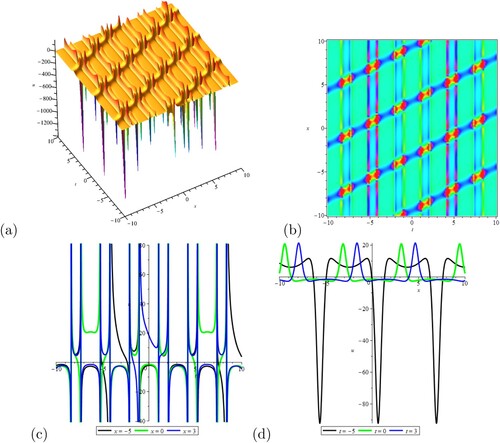and then we can receive Figure 2, which is periodic wave. (a) and (b) show the interaction of multiple waves, moving in the same direction and mode of propagation after a collision. Whether in the u-t plane or u-x plane, these solutions change periodically in (c) and (d).

Figure 2. The soliton wave solution gained from Equation (12(12) $\begin{array}{rl}U({\xi }_1,{\xi }_2)& =p_0(t)+p_{1,0}(t){\varphi }_1({\xi }_1)+p_{0,1}(t){\varphi }_2({\xi }_2)\\ & +p_{1,1}(t){\varphi }_1({\xi }_1){\varphi }_2({\xi }_2)+p_{2,0}(t){\varphi }_1^2({\xi }_1)\\ & +p_{0,2}(t){\varphi }_2^2({\xi }_2),\end{array}$(12) ) for ${\alpha }_1=1$, ${\beta }_1=-1$, ${\beta }_2=-1$, ${\sigma }_2(t)=1+2\cos (2t)$, $b_0(t)=-1$ and $c_0(t)=-1$. (a) of 3D-plot; (b) of contour plot; (c) of u-t plot; (d) of u-x plot.

2.3. The elliptic solutions

In the light of the method, we take into account the solutions of Equation (5(5) $\begin{array}{rl}& {\sigma }_1(t)(U_1{\alpha }_1+U_2{\beta }_1){\alpha }_1^2{U}_{11}+2{\sigma }_1(t)(U_1{\alpha }_1\\ & +U_2{\beta }_1){\alpha }_1{\beta }_1{U}_{12}+{\sigma }_1(t)(U_1{\alpha }_1+U_2{\beta }_1){\beta }_1^2{U}_{22}\\ & +{\sigma }_2(t)U{\alpha }_1^3{U}_{111}+3{\sigma }_2(t)U{\alpha }_1^2{\beta }_1{U}_{112}\\ & +3{\sigma }_2(t)U{\alpha }_1{\beta }_1^2{U}_{122}+3{\sigma }_2(t)U{\beta }_1^3{U}_{222}+{\alpha }_1^5{U}_{11111}\\ & {\sigma }_4(t)+5{\sigma }_4(t){\alpha }_1^4{\beta }_1{U}_{11112}+10{\sigma }_4(t){\alpha }_1^3{\beta }_1^2{U}_{11122}\\ & +10{\sigma }_4(t){\alpha }_1^2{\beta }_1^3{U}_{11222}+5{\sigma }_4(t){\alpha }_1{\beta }_1^4{U}_{12222}\\ & +U_1{\alpha }_2+U_2{\beta }_2+{\sigma }_3(t)(U_1{\alpha }_1+U_2{\beta }_1)U^2\\ & +{\sigma }_4(t){\beta }_1^5{U}_{22222}=0,\end{array}$(5) ) in the form (17) $\begin{array}{rl}U({\xi }_1,{\xi }_2)& =p_0(t)+p_{1,0}(t){\varphi }_1({\xi }_1)+p_{0,1}(t){\varphi }_2({\xi }_2)\\ & +p_{1,1}(t){\varphi }_1({\xi }_1){\varphi }_2({\xi }_2)+p_{2,0}(t){\varphi }_1^2({\xi }_1)\\ & +p_{0,2}(t){\varphi }_2^2({\xi }_2),\end{array}$(17) (18) $\begin{array}{rl}{\varphi }_1^{\prime }({\xi }_1)& =\sqrt{b_0(t)+b_2(t){\varphi }_1^2({\xi }_1)+b_4(t){\varphi }_1^4({\xi }_1)},\\ {\varphi }_2^{\prime }({\xi }_2)& =\sqrt{c_0(t)+c_2(t){\varphi }_2^2({\xi }_2)+c_4(t){\varphi }_2^4({\xi }_2)}.\end{array}$(18) By a similar way, we obtain (19) $\begin{array}{rl}& p_{1,1}(t)=0,p_{0,1}(t)=0,p_{1,0}(t)=0,\\ & {\sigma }_1(t)={\sigma }_2(t),p_{0,2}(t)=-{\displaystyle \frac{30{\sigma }_4(t){\beta }_1^2{c}_4(t)}{{\sigma }_2(t)}},\\ & p_{2,0}(t)=-{\displaystyle \frac{30{\sigma }_4(t){\alpha }_1^2{b}_4(t)}{{\sigma }_2(t)}},{\sigma }_3(t)={\displaystyle \frac{{\sigma }_2^2(t)}{5{\sigma }_4(t)}},\\ & p_0(t)=-{\displaystyle \frac{10{\sigma }_4(t)(b_2(t){\alpha }_1^2+c_2(t){\beta }_1^2)}{{\sigma }_2(t)}}.\end{array}$(19) Obviously, if the coefficients of Equation (18(18) $\begin{array}{rl}{\varphi }_1^{\prime }({\xi }_1)& =\sqrt{b_0(t)+b_2(t){\varphi }_1^2({\xi }_1)+b_4(t){\varphi }_1^4({\xi }_1)},\\ {\varphi }_2^{\prime }({\xi }_2)& =\sqrt{c_0(t)+c_2(t){\varphi }_2^2({\xi }_2)+c_4(t){\varphi }_2^4({\xi }_2)}.\end{array}$(18) ) are (20) $\begin{array}{rl}& b_0(t)=-{\displaystyle \frac{(1-m_1^2{)}^2}{4}},b_2(t)={\displaystyle \frac{1+m_1^2}{2}},\\ & b_4(t)=-{\displaystyle \frac{1}{4}},\\ & c_0(t)=-{\displaystyle \frac{(1-m_2^2{)}^2}{4}},c_2(t)={\displaystyle \frac{1+m_2^2}{2}},\\ & c_4(t)=-{\displaystyle \frac{1}{4}}.\end{array}$(20) The solutions of the auxiliary equations [35] in Equation (18(18) $\begin{array}{rl}{\varphi }_1^{\prime }({\xi }_1)& =\sqrt{b_0(t)+b_2(t){\varphi }_1^2({\xi }_1)+b_4(t){\varphi }_1^4({\xi }_1)},\\ {\varphi }_2^{\prime }({\xi }_2)& =\sqrt{c_0(t)+c_2(t){\varphi }_2^2({\xi }_2)+c_4(t){\varphi }_2^4({\xi }_2)}.\end{array}$(18) ) can be obtained (21) $\begin{array}{r}{\varphi }_1({\xi }_1)=m_1\text{cn}({\xi }_1,m_1)+\text{dn}({\xi }_1,m_1),\\ {\varphi }_2({\xi }_2)=m_2\text{cn}({\xi }_2,m_2)-\text{dn}({\xi }_2,m_2),\end{array}$(21) where $0<m_1<1$ and $0<m_2<1$.

Finally, the solution of Equation (1(1) $\begin{array}{rl}& u_t+{\sigma }_1(t)u_x{u}_{xx}+{\sigma }_2(t)u{u}_{xxx}+{\sigma }_3(t)u^2{u}_x\\ & +{\sigma }_4(t)u_{xxxxx}=0,\end{array}$(1) ) is (22) $\begin{array}{rl}{u}_3(x,t)& =-{\displaystyle \frac{5{\sigma }_4(t)({\alpha }_1^2{m}_1^2+{\beta }_1^2{m}_2^2+{\alpha }_1^2+{\beta }_1^2)}{{\sigma }_2(t)}}\\ & +{\displaystyle \frac{15{\sigma }_4(t){\alpha }_1^2(m_1\text{cn}({\xi }_1,m_1)+\text{dn}({\xi }_1,m_1){)}^2}{2{\sigma }_2(t)}}\\ & +{\displaystyle \frac{15{\sigma }_4(t){\beta }_1^2(m_2\text{cn}({\xi }_2,m_2)-\text{dn}({\xi }_2,m_2){)}^2}{2{\sigma }_2(t)}},\end{array}$(22) where ${\xi }_1={\alpha }_{1}x+{\alpha }_{2}t$, ${\xi }_1={\beta }_{1}x+{\beta }_{2}t$, $\begin{array}{rl}{\alpha }_2& =60{\alpha }_1(c_0(t)c_4(t){\beta }_1^4-{\displaystyle \frac{c_2^2(t){\beta }_1^4}{3}}\\ & -{\displaystyle \frac{b_0(t)b_4(t){\alpha }_1^4}{5}}+{\displaystyle \frac{b_2^2(t){\alpha }_1^4}{15}}){\sigma }_4(t)\end{array}$and $\begin{array}{rl}{\beta }_2& =-12{\beta }_1(c_0(t)c_4(t){\beta }_1^4-{\displaystyle \frac{c_2^2(t){\beta }_1^4}{3}}\\ & -5b_0(t)b_4(t){\alpha }_1^4+{\displaystyle \frac{5b_2^2(t){\alpha }_1^4}{3}}){\sigma }_4(t).\end{array}$

3. The modified Kudryashov method

In this part, we will employ the modified Kudryashov method to study and analyse the vcCDG equation. To solve Equation (1(1) $\begin{array}{rl}& u_t+{\sigma }_1(t)u_x{u}_{xx}+{\sigma }_2(t)u{u}_{xxx}+{\sigma }_3(t)u^2{u}_x\\ & +{\sigma }_4(t)u_{xxxxx}=0,\end{array}$(1) ), we need to make the following assumptions: (23) $u=U(\xi ),\xi ={\alpha }_{1}x+{\alpha }_{2}t,$(23) where ${\alpha }_1$ and ${\alpha }_2$ are arbitrary constants. By above transformation, Equation (1(1) $\begin{array}{rl}& u_t+{\sigma }_1(t)u_x{u}_{xx}+{\sigma }_2(t)u{u}_{xxx}+{\sigma }_3(t)u^2{u}_x\\ & +{\sigma }_4(t)u_{xxxxx}=0,\end{array}$(1) ) can be transformed into ordinary differential equation (24) $\begin{array}{rl}& U^{\prime }{\alpha }_2+{\sigma }_1(t){\alpha }_1^3{U}^{\prime }{U}^{″}+{\sigma }_2(t){\alpha }_1^{3}U{U}^{‴}+{\sigma }_3(t){\alpha }_1{U}^2{U}^{\prime }\\ & +{\sigma }_4(t){\alpha }_1^5{U}^{(5)}=0,\end{array}$(24) where $U^{\prime }=\frac{\text{d}U}{\text{d}\xi }$.

On the basis of the method, the layout of the solutions of Equation (24(24) $\begin{array}{rl}& U^{\prime }{\alpha }_2+{\sigma }_1(t){\alpha }_1^3{U}^{\prime }{U}^{″}+{\sigma }_2(t){\alpha }_1^{3}U{U}^{‴}+{\sigma }_3(t){\alpha }_1{U}^2{U}^{\prime }\\ & +{\sigma }_4(t){\alpha }_1^5{U}^{(5)}=0,\end{array}$(24) ) can be set (25) $U(\xi )=\sum _0^N{q}_i(t){\varphi }^i(\xi ),$(25) where the auxiliary equation with regard to x is (26) ${\varphi }^{\prime }(\xi )={\varphi }^2(\xi )-\varphi (\xi ).$(26) Therefore, the first thing we need to do is to calculate the value of N. After that we can determine the specific form of the solution of Equation (24(24) $\begin{array}{rl}& U^{\prime }{\alpha }_2+{\sigma }_1(t){\alpha }_1^3{U}^{\prime }{U}^{″}+{\sigma }_2(t){\alpha }_1^{3}U{U}^{‴}+{\sigma }_3(t){\alpha }_1{U}^2{U}^{\prime }\\ & +{\sigma }_4(t){\alpha }_1^5{U}^{(5)}=0,\end{array}$(24) ). Similarly, N can be obtained by balancing $U^{(5)}$ and $U^2{U}^{\prime }$ in Equation (24(24) $\begin{array}{rl}& U^{\prime }{\alpha }_2+{\sigma }_1(t){\alpha }_1^3{U}^{\prime }{U}^{″}+{\sigma }_2(t){\alpha }_1^{3}U{U}^{‴}+{\sigma }_3(t){\alpha }_1{U}^2{U}^{\prime }\\ & +{\sigma }_4(t){\alpha }_1^5{U}^{(5)}=0,\end{array}$(24) ), we compute (27) $N=2.$(27) Therefore, we can get the exact form of Equation (25(25) $U(\xi )=\sum _0^N{q}_i(t){\varphi }^i(\xi ),$(25) ) is (28) $U(\xi )=q_0(t)+q_1(t)\varphi (\xi )+q_2(t){\varphi }^2(\xi ).$(28) According to this method, we need to bring Equations (26(26) ${\varphi }^{\prime }(\xi )={\varphi }^2(\xi )-\varphi (\xi ).$(26) ) and (28(28) $U(\xi )=q_0(t)+q_1(t)\varphi (\xi )+q_2(t){\varphi }^2(\xi ).$(28) ) together into Equation (24(24) $\begin{array}{rl}& U^{\prime }{\alpha }_2+{\sigma }_1(t){\alpha }_1^3{U}^{\prime }{U}^{″}+{\sigma }_2(t){\alpha }_1^{3}U{U}^{‴}+{\sigma }_3(t){\alpha }_1{U}^2{U}^{\prime }\\ & +{\sigma }_4(t){\alpha }_1^5{U}^{(5)}=0,\end{array}$(24) ). And by combining the same terms, we can get a series of equations of $\varphi (\xi )$ and make each coefficient of $\varphi (\xi )$ equal to zero. Finally, according to the above steps and symbolic calculation, we can acquire the following four solutions:

Case 1: (29) $\begin{array}{rl}& {\sigma }_1(t)={\displaystyle \frac{-{\sigma }_2^2(t)+10{\sigma }_3(t){\sigma }_4(t)}{{\sigma }_2(t)}},q_1(t)={\displaystyle \frac{6{\alpha }_1^2{\sigma }_2(t)}{{\sigma }_3(t)}},\\ & q_2(t)=-{\displaystyle \frac{6{\alpha }_1^2{\sigma }_2(t)}{{\sigma }_3(t)}},\\ & {\alpha }_2=-{\alpha }_1^5{\sigma }_4(t)-q_0(t){\sigma }_2(t){\alpha }_1^3-q_0^2(t){\sigma }_3(t){\alpha }_1.\end{array}$(29) Then, putting Equation (29(29) $\begin{array}{rl}& {\sigma }_1(t)={\displaystyle \frac{-{\sigma }_2^2(t)+10{\sigma }_3(t){\sigma }_4(t)}{{\sigma }_2(t)}},q_1(t)={\displaystyle \frac{6{\alpha }_1^2{\sigma }_2(t)}{{\sigma }_3(t)}},\\ & q_2(t)=-{\displaystyle \frac{6{\alpha }_1^2{\sigma }_2(t)}{{\sigma }_3(t)}},\\ & {\alpha }_2=-{\alpha }_1^5{\sigma }_4(t)-q_0(t){\sigma }_2(t){\alpha }_1^3-q_0^2(t){\sigma }_3(t){\alpha }_1.\end{array}$(29) ) into Equation (28(28) $U(\xi )=q_0(t)+q_1(t)\varphi (\xi )+q_2(t){\varphi }^2(\xi ).$(28) ), the solution of Equation (24(24) $\begin{array}{rl}& U^{\prime }{\alpha }_2+{\sigma }_1(t){\alpha }_1^3{U}^{\prime }{U}^{″}+{\sigma }_2(t){\alpha }_1^{3}U{U}^{‴}+{\sigma }_3(t){\alpha }_1{U}^2{U}^{\prime }\\ & +{\sigma }_4(t){\alpha }_1^5{U}^{(5)}=0,\end{array}$(24) ) can be found (30) $\begin{array}{rl}{u}_4(x,t)& ={\displaystyle \frac{1}{2{\sigma }_3(t)}}\\ & \times (-3{\tanh }^2\left({\displaystyle \frac{\begin{array}{c}{\alpha }_1(t{\alpha }_1^4{\sigma }_4(t)\\ +q_0(t){\sigma }_2(t){\alpha }_1^{2}t\\ +q_0^2(t){\sigma }_3(t)t-x)\end{array}}{2}}\right){\sigma }_2(t){\alpha }_1^2\\ & \phantom{\left({\displaystyle \frac{\begin{array}{c}{\alpha }_1(t{\alpha }_1^4{\sigma }_4(t)\\ +q_0(t){\sigma }_2(t){\alpha }_1^{2}t\\ +q_0^2(t){\sigma }_3(t)t-x)\end{array}}{2}}\right)}+3{\alpha }_1^2{\sigma }_2(t)+q_0(t){\sigma }_3(t)).\end{array}$(30) Finally, we assign values to the parameters in the above solution. 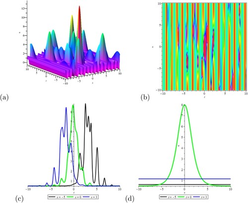When the parameters ${\alpha }_1=1-2\cos (3t)$, $q_0(t)=\frac{1}{2}+\sin (5t)$, ${\sigma }_2(t)=-5+\sin (4t)$, ${\sigma }_3(t)=-1$ and ${\sigma }_4(t)=1+3\cos (t)$, we can get Figure 3. They show the interaction between multiple bright soliton waves in (a) and (b). Obviously, the solutions in (c) change greatly. In (d), the value of u changes greatly, and then it turns to be gradual after a sharp change.

Figure 3. The travelling wave solution given by Equation (30(30) $\begin{array}{rl}{u}_4(x,t)& ={\displaystyle \frac{1}{2{\sigma }_3(t)}}\\ & \times (-3{\tanh }^2\left({\displaystyle \frac{\begin{array}{c}{\alpha }_1(t{\alpha }_1^4{\sigma }_4(t)\\ +q_0(t){\sigma }_2(t){\alpha }_1^{2}t\\ +q_0^2(t){\sigma }_3(t)t-x)\end{array}}{2}}\right){\sigma }_2(t){\alpha }_1^2\\ & \phantom{\left({\displaystyle \frac{\begin{array}{c}{\alpha }_1(t{\alpha }_1^4{\sigma }_4(t)\\ +q_0(t){\sigma }_2(t){\alpha }_1^{2}t\\ +q_0^2(t){\sigma }_3(t)t-x)\end{array}}{2}}\right)}+3{\alpha }_1^2{\sigma }_2(t)+q_0(t){\sigma }_3(t)).\end{array}$(30) ) at ${\alpha }_1=1-2\cos (3t)$, $q_0(t)=\frac{1}{2}+\sin (5t)$, ${\sigma }_2(t)=-5+\sin (4t)$, ${\sigma }_3(t)=-1$ and ${\sigma }_4(t)=1+3\cos (t)$. (a) of 3D-plot; (b) of contour plot; (c) of u-t plot; (d) of u-x plot.

Case 2: (31) $\begin{array}{rl}& {\sigma }_3(t)={\displaystyle \frac{{\sigma }_2^2(t)+{\sigma }_1(t){\sigma }_2(t)}{10{\sigma }_4(t)}},\\ & q_1(t)={\displaystyle \frac{60{\alpha }_1^2{\sigma }_4(t)}{{\sigma }_1(t)+{\sigma }_2(t)}},\\ & q_2(t)=-{\displaystyle \frac{60{\alpha }_1^2{\sigma }_4(t)}{{\sigma }_1(t)+{\sigma }_2(t)}},\\ & {\alpha }_2=-{\displaystyle \frac{\begin{array}{c}{\alpha }_1(\frac{({\sigma }_1(t)+{\sigma }_2(t)){\sigma }_2(t)q_0^2(t)}{10}\\ +{\sigma }_2(t)q_0(t){\alpha }_1^2{\sigma }_4(t)+{\alpha }_1^4{\sigma }_4^2(t))\end{array}}{{\sigma }_4(t)}}.\end{array}$(31) Inserting Equation (31(31) $\begin{array}{rl}& {\sigma }_3(t)={\displaystyle \frac{{\sigma }_2^2(t)+{\sigma }_1(t){\sigma }_2(t)}{10{\sigma }_4(t)}},\\ & q_1(t)={\displaystyle \frac{60{\alpha }_1^2{\sigma }_4(t)}{{\sigma }_1(t)+{\sigma }_2(t)}},\\ & q_2(t)=-{\displaystyle \frac{60{\alpha }_1^2{\sigma }_4(t)}{{\sigma }_1(t)+{\sigma }_2(t)}},\\ & {\alpha }_2=-{\displaystyle \frac{\begin{array}{c}{\alpha }_1(\frac{({\sigma }_1(t)+{\sigma }_2(t)){\sigma }_2(t)q_0^2(t)}{10}\\ +{\sigma }_2(t)q_0(t){\alpha }_1^2{\sigma }_4(t)+{\alpha }_1^4{\sigma }_4^2(t))\end{array}}{{\sigma }_4(t)}}.\end{array}$(31) ) into Equation (28(28) $U(\xi )=q_0(t)+q_1(t)\varphi (\xi )+q_2(t){\varphi }^2(\xi ).$(28) ), we obtain the following solution of Equation (24(24) $\begin{array}{rl}& U^{\prime }{\alpha }_2+{\sigma }_1(t){\alpha }_1^3{U}^{\prime }{U}^{″}+{\sigma }_2(t){\alpha }_1^{3}U{U}^{‴}+{\sigma }_3(t){\alpha }_1{U}^2{U}^{\prime }\\ & +{\sigma }_4(t){\alpha }_1^5{U}^{(5)}=0,\end{array}$(24) ), (32) $\begin{array}{rl}{u}_5(x,t)& =\frac{1}{{\sigma }_1(t)+{\sigma }_2(t)}\\ & \times (\phantom{\left(\frac{\begin{array}{c}{\alpha }_1(10t{\alpha }_1^4{\sigma }_4^2(t)\\ +10p_0(t){\sigma }_2(t){\alpha }_1^{2}t{\sigma }_4(t)\\ +q_0^2(t){\sigma }_2^2(t)t+{\sigma }_2(t)q_0^2(t){\sigma }_1(t)t\\ -10{\sigma }_4(t)x)\end{array}}{20{\sigma }_4(t)}\right)}15{\alpha }_1^2{\sigma }_4(t)+q_0(t)({\sigma }_1(t)+{\sigma }_2(t))\\ & \times {\tanh }^2\left(\frac{\begin{array}{c}{\alpha }_1(10t{\alpha }_1^4{\sigma }_4^2(t)\\ +10p_0(t){\sigma }_2(t){\alpha }_1^{2}t{\sigma }_4(t)\\ +q_0^2(t){\sigma }_2^2(t)t+{\sigma }_2(t)q_0^2(t){\sigma }_1(t)t\\ -10{\sigma }_4(t)x)\end{array}}{20{\sigma }_4(t)}\right)\\ & \times \phantom{\left(\frac{\begin{array}{c}{\alpha }_1(10t{\alpha }_1^4{\sigma }_4^2(t)\\ +10p_0(t){\sigma }_2(t){\alpha }_1^{2}t{\sigma }_4(t)\\ +q_0^2(t){\sigma }_2^2(t)t+{\sigma }_2(t)q_0^2(t){\sigma }_1(t)t\\ -10{\sigma }_4(t)x)\end{array}}{20{\sigma }_4(t)}\right)}(-15{\sigma }_4(t){\alpha }_1^2)).\end{array}$(32) On the basis of the above solution, if we take ${\alpha }_1=1-2\tan (3t)$, $q_0(t)=\frac{1}{2}+3\sin (2t)$, ${\sigma }_1(t)=-\frac{1}{2}$, ${\sigma }_2(t)=5+2\sin (4t)$ and ${\sigma }_4(t)=1+8\cos (3t)$, 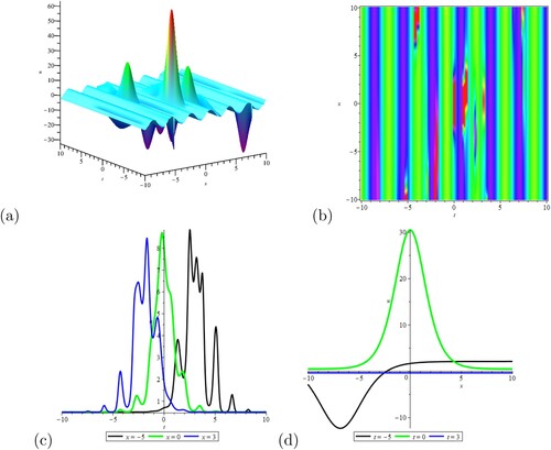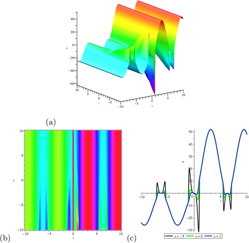we obtain Figure 4. It shows the fluid-lattice wave solutions. We see that the rogue waves owing to the interaction between kinky and anti-kinky periodic waves in (a) and (b). The value of u varies greatly in (c). In (d), the solutions change dramatically when $t=0$, $-5<x<5$ and $t=-5$, $-10<x<0$.

Figure 4. The travelling wave solution calculated by Equation (32(32) $\begin{array}{rl}{u}_5(x,t)& =\frac{1}{{\sigma }_1(t)+{\sigma }_2(t)}\\ & \times (\phantom{\left(\frac{\begin{array}{c}{\alpha }_1(10t{\alpha }_1^4{\sigma }_4^2(t)\\ +10p_0(t){\sigma }_2(t){\alpha }_1^{2}t{\sigma }_4(t)\\ +q_0^2(t){\sigma }_2^2(t)t+{\sigma }_2(t)q_0^2(t){\sigma }_1(t)t\\ -10{\sigma }_4(t)x)\end{array}}{20{\sigma }_4(t)}\right)}15{\alpha }_1^2{\sigma }_4(t)+q_0(t)({\sigma }_1(t)+{\sigma }_2(t))\\ & \times {\tanh }^2\left(\frac{\begin{array}{c}{\alpha }_1(10t{\alpha }_1^4{\sigma }_4^2(t)\\ +10p_0(t){\sigma }_2(t){\alpha }_1^{2}t{\sigma }_4(t)\\ +q_0^2(t){\sigma }_2^2(t)t+{\sigma }_2(t)q_0^2(t){\sigma }_1(t)t\\ -10{\sigma }_4(t)x)\end{array}}{20{\sigma }_4(t)}\right)\\ & \times \phantom{\left(\frac{\begin{array}{c}{\alpha }_1(10t{\alpha }_1^4{\sigma }_4^2(t)\\ +10p_0(t){\sigma }_2(t){\alpha }_1^{2}t{\sigma }_4(t)\\ +q_0^2(t){\sigma }_2^2(t)t+{\sigma }_2(t)q_0^2(t){\sigma }_1(t)t\\ -10{\sigma }_4(t)x)\end{array}}{20{\sigma }_4(t)}\right)}(-15{\sigma }_4(t){\alpha }_1^2)).\end{array}$(32) ) with ${\alpha }_1=1-2\tan (3t)$, $q_0(t)=\frac{1}{2}+3\sin (2t)$, ${\sigma }_1(t)=-\frac{1}{2}$, ${\sigma }_2(t)=5+2\sin (4t)$ and ${\sigma }_4(t)=1+8\cos (3t)$. (a) of 3D-plot; (b) of contour plot; (c) of u-t plot; (d) of u-x plot.

Case 3: (33) $\begin{array}{rl}& {\sigma }_4(t)={\displaystyle \frac{(-15+\sqrt{849}){\alpha }_2}{546{\alpha }_1^5}},\\ & {\sigma }_3(t)={\displaystyle \frac{252(-181+6\sqrt{849}){\alpha }_1^5{\sigma }_2^2(t)}{13{\alpha }_2(-15+\sqrt{849})}},\\ & q_0(t)=-{\displaystyle \frac{(-15+\sqrt{849}){\alpha }_2}{42{\alpha }_1^3{\sigma }_2(t)}},\\ & q_2(t)=-{\displaystyle \frac{2(-15+\sqrt{849}{)}^2{\alpha }_2}{7{\alpha }_1^3{\sigma }_2(t)(-183+7\sqrt{849})}},\\ & {\sigma }_1(t)=-{\displaystyle \frac{(-3147+137\sqrt{849}){\sigma }_2(t)}{-390+26\sqrt{849}}},q_1(t)=0.\end{array}$(33) We also take Equation (33(33) $\begin{array}{rl}& {\sigma }_4(t)={\displaystyle \frac{(-15+\sqrt{849}){\alpha }_2}{546{\alpha }_1^5}},\\ & {\sigma }_3(t)={\displaystyle \frac{252(-181+6\sqrt{849}){\alpha }_1^5{\sigma }_2^2(t)}{13{\alpha }_2(-15+\sqrt{849})}},\\ & q_0(t)=-{\displaystyle \frac{(-15+\sqrt{849}){\alpha }_2}{42{\alpha }_1^3{\sigma }_2(t)}},\\ & q_2(t)=-{\displaystyle \frac{2(-15+\sqrt{849}{)}^2{\alpha }_2}{7{\alpha }_1^3{\sigma }_2(t)(-183+7\sqrt{849})}},\\ & {\sigma }_1(t)=-{\displaystyle \frac{(-3147+137\sqrt{849}){\sigma }_2(t)}{-390+26\sqrt{849}}},q_1(t)=0.\end{array}$(33) ) into Equation (28(28) $U(\xi )=q_0(t)+q_1(t)\varphi (\xi )+q_2(t){\varphi }^2(\xi ).$(28) ), and then we have (34) $\begin{array}{rl}{u}_6(x,t)& ={\displaystyle \frac{(-15+\sqrt{849}){\alpha }_2}{14{\alpha }_1^3{\sigma }_2(t)(-183+7\sqrt{849})}}\\ & \times (\phantom{{\displaystyle \frac{4\sqrt{849}}{3}}}(-15+\sqrt{849}){\tanh }^2({\displaystyle \frac{{\alpha }_{2}t}{2}}+{\displaystyle \frac{{\alpha }_{1}x}{2}})\\ & +(30-2\sqrt{849}){\tanh }^2({\displaystyle \frac{{\alpha }_{2}t}{2}}+{\displaystyle \frac{{\alpha }_{1}x}{2}})\\ & +46-{\displaystyle \frac{4\sqrt{849}}{3}}).\end{array}$(34) Figure 5 shows that the solution of Equation (24(24) $\begin{array}{rl}& U^{\prime }{\alpha }_2+{\sigma }_1(t){\alpha }_1^3{U}^{\prime }{U}^{″}+{\sigma }_2(t){\alpha }_1^{3}U{U}^{‴}+{\sigma }_3(t){\alpha }_1{U}^2{U}^{\prime }\\ & +{\sigma }_4(t){\alpha }_1^5{U}^{(5)}=0,\end{array}$(24) ) when ${\alpha }_1=-10-5\cos (5t)$, ${\alpha }_2=-1+8\tanh (3t)$ and ${\sigma }_2(t)=-6+5\sin (5t)$. Figure 5 presents the elastic collision between multiple periodic waves in (a) and (b). In (c) when $t>0$, the amplitude is larger and changes faster. The value of u changes sharply near $x=3$ in (d).

Figure 5. The travelling wave solution given by Equation (34(34) $\begin{array}{rl}{u}_6(x,t)& ={\displaystyle \frac{(-15+\sqrt{849}){\alpha }_2}{14{\alpha }_1^3{\sigma }_2(t)(-183+7\sqrt{849})}}\\ & \times (\phantom{{\displaystyle \frac{4\sqrt{849}}{3}}}(-15+\sqrt{849}){\tanh }^2({\displaystyle \frac{{\alpha }_{2}t}{2}}+{\displaystyle \frac{{\alpha }_{1}x}{2}})\\ & +(30-2\sqrt{849}){\tanh }^2({\displaystyle \frac{{\alpha }_{2}t}{2}}+{\displaystyle \frac{{\alpha }_{1}x}{2}})\\ & +46-{\displaystyle \frac{4\sqrt{849}}{3}}).\end{array}$(34) ) when ${\alpha }_1=-10-5\cos (5t)$, ${\alpha }_2=-1+8\tanh (3t)$ and ${\sigma }_2(t)=-6+5\sin (5t)$. (a) of 3D-plot; (b) of contour plot; (c) of u-t plot; (d) of u-x plot.

Case 4: (35) $\begin{array}{rl}& {\sigma }_3(t)=-{\displaystyle \frac{(-187+7\sqrt{849}){\sigma }_2^2(t)}{1352{\sigma }_4(t)}},\\ & q_0(t)=-{\displaystyle \frac{13{\alpha }_1^2{\sigma }_4(t)}{{\sigma }_2(t)}},\\ & q_1(t)=0,{\sigma }_1(t)={\displaystyle \frac{7\sqrt{849}{\sigma }_2(t)}{104}}-{\displaystyle \frac{443{\sigma }_2(t)}{104}},\\ & q_2(t)=-{\displaystyle \frac{1248{\alpha }_1^2{\sigma }_4(t)}{{\sigma }_2(t)(-41+\sqrt{849})}},\\ & {\alpha }_2={\displaystyle \frac{7(15+\sqrt{849}){\alpha }_1^5{\sigma }_4(t)}{8}}.\end{array}$(35) And then, we have (36) $\begin{array}{rl}{u}_7(x,t)& =-{\displaystyle \frac{1}{{\sigma }_2(t)(-41+\sqrt{849})}}\\ & \times (-48\tanh ({\displaystyle \frac{105t{\alpha }_1^5{\sigma }_4(t)}{15}}\\ & +{\displaystyle \frac{7t{\alpha }_1^5{\sigma }_4(t)\sqrt{849}}{16}}+{\displaystyle \frac{{\alpha }_{1}x}{2}})\\ & -17+\sqrt{849}+24{\tanh }^2\\ & \times ({\displaystyle \frac{105t{\alpha }_1^5{\sigma }_4(t)}{15}}\\ & +{\displaystyle \frac{7t{\alpha }_1^5{\sigma }_4(t)\sqrt{849}}{16}}+{\displaystyle \frac{{\alpha }_{1}x}{2}})13{\sigma }_4(t){\alpha }_1^2).\end{array}$(36) In Equation (36(36) $\begin{array}{rl}{u}_7(x,t)& =-{\displaystyle \frac{1}{{\sigma }_2(t)(-41+\sqrt{849})}}\\ & \times (-48\tanh ({\displaystyle \frac{105t{\alpha }_1^5{\sigma }_4(t)}{15}}\\ & +{\displaystyle \frac{7t{\alpha }_1^5{\sigma }_4(t)\sqrt{849}}{16}}+{\displaystyle \frac{{\alpha }_{1}x}{2}})\\ & -17+\sqrt{849}+24{\tanh }^2\\ & \times ({\displaystyle \frac{105t{\alpha }_1^5{\sigma }_4(t)}{15}}\\ & +{\displaystyle \frac{7t{\alpha }_1^5{\sigma }_4(t)\sqrt{849}}{16}}+{\displaystyle \frac{{\alpha }_{1}x}{2}})13{\sigma }_4(t){\alpha }_1^2).\end{array}$(36) ), given the parameters ${\alpha }_1=1-\cos (t)$, ${\sigma }_2(t)=-2+2\cos (t)$ and ${\sigma }_4(t)=1+3\tanh (5t)$, we get the Figure 6. It illustrates that periodic wave and solitary wave for two different velocities combine into a rogue wave in (a) and (b). It is antisymmetric, and when $t=0$, the value of u is also 0 in (c).

Figure 6. The travelling wave solution given by Equation (36(36) $\begin{array}{rl}{u}_7(x,t)& =-{\displaystyle \frac{1}{{\sigma }_2(t)(-41+\sqrt{849})}}\\ & \times (-48\tanh ({\displaystyle \frac{105t{\alpha }_1^5{\sigma }_4(t)}{15}}\\ & +{\displaystyle \frac{7t{\alpha }_1^5{\sigma }_4(t)\sqrt{849}}{16}}+{\displaystyle \frac{{\alpha }_{1}x}{2}})\\ & -17+\sqrt{849}+24{\tanh }^2\\ & \times ({\displaystyle \frac{105t{\alpha }_1^5{\sigma }_4(t)}{15}}\\ & +{\displaystyle \frac{7t{\alpha }_1^5{\sigma }_4(t)\sqrt{849}}{16}}+{\displaystyle \frac{{\alpha }_{1}x}{2}})13{\sigma }_4(t){\alpha }_1^2).\end{array}$(36) ) for ${\alpha }_1=1-\cos (t)$, ${\sigma }_2(t)=-2+2\cos (t)$ and ${\sigma }_4(t)=1+3\tanh (5t)$. (a) of 3D-plot; (b) of contour plot; (c) of u-t plot.

4. Conclusions

Here, the vcCDG equation is studied and analysed by the unified method and the modified Kudryashov method. Compared with other methods, we receive more different travelling wave solutions and classify some solutions like solitary wave solutions, soliton wave solutions and elliptic wave solutions. These solutions contribute to a better understanding of physics phenomena in different branches of engineering science, mathematical physics, quantum mechanics and nonlinear optics, and other technical fields. By choosing appropriate parameters, 3D and 2D plots of some solutions are plotted, from which we are able to obtain periodic waves, rogue waves and kink solitary waves. Through these, we can get more physical meaning of the cvCDG equation. The unified method and the modified Kudryashov method are significant in the study of solutions of nonlinear partial differential equations, have good research prospect and also provide an idea and direction for solving other problems.

Disclosure statement

No potential conflict of interest was reported by the author(s).

Additional information

Funding

This work was supported by the Natural Science Foundation of Shanxi [grant number 202103021224068].

References

- Chentouf B. On the exponential stability of a nonlinear Kuramoto–Sivashinsky–Korteweg–de Vries equation with finite memory. Mediterr J Math. 2022;19:11.
- Chentouf B. Well-posedness and exponential stability results for a nonlinear Kuramoto–Sivashinsky equation with a boundary time-delay. Anal Math Phys. 2021;11:144.
- Chentouf B. Qualitative analysis of the dynamic for the nonlinear Korteweg–de Vries equation with a boundary memory. Qual Theory Dyn Syst. 2021;20:36.
- Chentouf B, Guesmia A. Well-posedness and stability results for the Korteweg–de Vries-Burgers and Kuramoto–Sivashinsky equations with infinite memory: a history approach. Nonlinear Anal Real World Appl. 2022;65:103–508.
- Ammari K, Chentouf B, Smaoui N. Well-posedness and stability of a nonlinear time-delayed dispersive equation via the fixed-point technique: a case study of no interior damping. Math Methods Appl Sci. 2022;45:4555–4566.
- Alam MN, Tunç C. The new solitary wave structures for the (2 + 1)-dimensional time-fractional Schrodinger equation and the space-time nonlinear conformable fractional Bogoyavlenskii equations. Alex Eng J. 2020;59:2221–2232.
- Islam S, Alam MN, Al-Asad MF, et al. An analytical technique for solving new computational of the modified Zakharov–Kuznetsov equation arising in electrical engineering. J Appl Comput Mech. 2021;7:715–726.
- Alam MN, Tunç C. Constructions of the optical solitons and others soliton to the conformable fractional Zakharov–Kuznetsov equation with power law nonlinearity. J Taibah Univ Sci. 2020;14:94–100.
- Alam N, Tunç C. New solitary wave structures to the (2 + 1)-dimensional KD and KP equations with spatio-temporal dispersion. J King Saud Univ Sci. 2020;32:3400–3409.
- Kumar D, Kaplan M. Application of the modified Kudryashov method to the generalized Schrdinger–Boussinesq equations. Opt Quantum Electron. 2018;50:329.
- Hosseini K, Mayeli P, Ansari R. Modified Kudryashov method for solving the conformable time-fractional Klein–Gordon equations with quadratic and cubic nonlinearities. Optik. 2016;130:737–742.
- Selvaraj R, Venkatraman S, Ashok DD, et al. Exact solutions of time-fractional generalised Burgers–Fisher equation using generalised Kudryashov method. Pramana. 2020;94:1–8.
- Adem AR, Yildirim Y, Yaşar E. Soliton solutions to the non-local Boussinesq equation by multiple exp-function scheme and extended Kudryashov's approach. Pramana. 2019;92:24.
- Ismail A. A discrete generalization of the extended simplest equation method. Commun Nonlinear Sci Numer Simul. 2010;15:1967–1973.
- Sudao Bilige A, Temuer Chaolu B, Xiaomin Wang A. Application of the extended simplest equation method to the coupled Schrdinger–Boussinesq equation. Appl Math Comput. 2013;224:517–523.
- Yang Y. Exact solutions of the Boussinesq equation using the extended simplest equation method. IOP Conf Ser Mater Sci Eng. 2019;677:42–72.
- Noeiaghdam S, Zarei E, Kelishami HB. Homotopy analysis transform method for solving Abel's integral equations of the first kind. Ain Shams Eng J. 2015;7:483–495.
- Abdel-Gawad HI. Towards a unified method for exact solutions of evolution equations. An application to reaction diffusion equations with finite memory transport. J Stat Phys. 2012;147:506–518.
- Yusuf A, Sulaiman TA, Inc M, et al. Breather wave, lump-periodic solutions and some other interaction phenomena to the Caudrey–Dodd–Gibbon equation. Eur Phys J Plus. 2020;135:563.
- Xu YG, Zhou XW, Li Y. Solving the fifth order Caudrey–Dodd–Gibbon (CDG) equation using the exp-function method. Appl Math Comput. 2008;206:70–73.
- Neamaty A, Agheli B, Darzi R. Exact travelling wave solutions for some nonlinear time fractional fifth-order Caudrey–Dodd–Gibbon equation by (g′/g)-expansion method. SeMA J. 2015;73:121–129.
- Kumar D, Kumar S. Some more solutions of Caudrey–Dodd–Gibbon equation using optimal system of lie symmetries. Int J Appl Comput Math. 2020;6:125.
- Jin L. Application of the variational iteration method for solving the fifth order Caudrey-Dodd–Gibbon equation. Oncogene. 2010;66:3259–3265.
- Bibi S, Ahmed N, Faisal I, et al. Some new solutions of the Caudrey–Dodd–Gibbon (CDG) equation using the conformable derivative. Adv Differ Equ. 2019;2019:1–27.
- Ahmad J, Nauman R, Osman MS. Multi-solitons of thermophoretic motion equation depicting the wrinkle propagation in substrate-supported graphene sheets. Commun Theor Phys. 2019;71:362.
- Osman MS, Baleanu D, Adem AR, et al. Double-wave solutions and lie symmetry analysis to the (2 + 1)-dimensional coupled burgers equations. Chinese J Phys. 2020;63:122–129.
- Osman MS, Rezazadeh H, Eslami M. Traveling wave solutions for (3 + 1) dimensional conformable fractional Zakharov-Kuznetsov equation with power law nonlinearity. Nonlinear Eng. 2019;8:559–567.
- Osman MS, Rezazadeh H, Eslami M, et al. Analytical study of solitons to Benjamin–Bona–Mahony–Peregrine equation with power law nonlinearity by using three methods. U Politeh Buch Ser A. 2018;80:187–267.
- Huai-Tang C, Hong-Qing Z. New double periodic and multiple soliton solutions of the generalized (2 + 1)-dimensional Boussinesq equation. Chaos Soliton Fract. 2014;20:765–769.
- Ray SS. New analytical exact solutions of time fractional KdV–KZK equation by Kudryashov methods. Chinese Phys B. 2016;25:40–204.
- Qu QX, Tian B, Sun K, et al. Bcklund transformation, lax pair, and solutions for the Caudrey–Dodd–Gibbon equation. J Math Phys. 2011;52:013511.
- Wazwaz AM. N-soliton solutions for the combined KdV–CDG equation and the KdV–Lax equation. Appl Math Comput. 2008;203:402–407.
- Tu JM, Tian SF, Xu MJ, et al. Quasi-periodic waves and solitary waves to a generalized KdV-Caudrey–Dodd–Gibbon equation from fluid dynamics. Taiwan J Math. 2016;20:823–848.
- Alam MK, Hossain MD, Akbar MA, et al. Determination of the rich structural wave dynamic solutions to the Caudrey–Dodd–Gibbon equation and the lax equation. Lett Math Phys. 2021;111:103.
- Osman MS, Abdel-Gawad HI. Multi-wave solutions of the (2 + 1)-dimensional Nizhnik–Novikov–Veselov equations with variable coefficients. Eur Phys J Plus. 2015;130:1–11.