Numerical treatment of some fractional nonlinear equations by Elzaki transform

ABSTRACT

This study solves systems of partial differential equations with fractional-order derivatives using a modified decomposition approach. Fractional-order derivatives are expressed using the Caputo operator. The validity of the suggested technique is tested using illustrative cases. The exact and Elzaki Adomian decomposition method (EADM) solutions were in close proximity, according to the solution graphs. The suggested strategy’s dependability is shown by the fact that fractional-order problems tend to converge on the solution to an integer-order problem. The present approach may be utilized to answer a broad variety of fractional-order issues since it is more precise and simple to use. Finally, some examples show how the new strategy is uncomplicated, effective, and precise. The approximate solutions have also been displayed at the conclusion of this study.

KEYWORDS:

• Caputo operator
• Adomian decomposition mothed
• Elzaki transformation
• fractional systems of partial differential equations

1. Introduction

Since nonlinearity is prevalent in practically all physical circumstances, scientists and engineers have focused a lot of attention on nonlinear equations in the last decade. In chemistry, biology, physics, vibration, acoustics, signal processing, electromagnetics, polymeric materials, and fluid dynamics, as well as superconductivity, optics, and quantum mechanics, nonlinear partial differential equations of fractional order are applied [1–5].

The most frequently developing field in mathematical analysis is fractional-order calculus. In actuality, fractional-order ordinary differential equations are utilized to model a wide range of physical processes that are dependent on time instants and earlier in time history. fractional-order partial differential equations (FODEs), and as a consequence, FDEs have grown more essential in a number of fields. Many studies have focused on fractional partial differential equations (FDEs) because of their importance [6–9].

Analytical and numerical solutions are available for FDEs [10–12]. A variety of approaches have been considered for the solution of FPDEs in this case, Homotopy perturbation methodology (HPM), Elzaki transformation, ordinary differential equation approach, variational approach, rectified Fourier series, and natural decomposition method [13–16]. Transformations of fractional complexity [17,18] investigates the optimum q-HAM for solving FPDEs. In [19], the Bernoulli wavelets and the collocation technique were employed to solve FPDEs effectively. The development of studying the dynamic behaviour of the drinking population by using the fractional- order operator in the Caputo–Fabrizio sense with a nonsingular kernel; the effect of memory, specifically the Caputo–Fabrizio time-fractional derivative on the solute concentration, is studied and compared with the traditional case; and the development of studying the dynamic behaviour of the drinking population by using the fractional drinking model in the sense of the thresh [20–22].

The supplementary Elzaki parameter technique [23] has been suggested for the solution of FDEs. The Kodomtsev–Petviashvili problem is solved using the simple equation approach in [24,2] provides a modified variational iteration strategy for the solution of nonlinear PDEs. The iterative Elzaki transform approach was used to examine the solution of linear and nonlinear FPDEs in [25]. Biological nonlinear phenomena that may be modelled using nonlinear PDEs of integer order include shallow water waves and multicellular biological dynamics [26]. In many FPDEs, numerical techniques are employed as a replacement for accurate or analytical solutions. For an explanation of shock wave occurrences in plasma, including charged dust particles, consider the Zakharov-Kuznetsov Burgers equation. A similarity transformation converts a set of partial differential equations into a set of ordinary differential equations. The given nonlinear model is turned into an ordinary differential equation by using a wave frame [27–30].

The tau approximation was used to generate numerical solutions to FPDEs in this context [31]. For solving linear and nonlinear FPDEs, discrete HAM is recommended [32–34]. The Laplace–Adomian decomposition method is a simple and efficient methodology for solving nonlinear FPDEs. Laplace Adomian decomposition method (LADM) is the result of combining the Elzaki transformation with the Adomian decomposition method (ADM). Unlike RK4, the recommended approach does not need a certain declaration size. In comparison to other analytical methodologies, LADM requires fewer parameters, no discretization, and no linearization [35]. In, LADM is compared to ADM to evaluate the solution of FPDEs provided in [36,37] proposes utilizing LADM to solve the Kundu–Eckhaus dilemma. In order to solve FPDEs, a multistep LADM is used [38,39]. In addition to fractional Navier–Stokes, smoke models, and third-order dispersive PDEs, LADM and EADM can solve them [40–42].

In this paper, we use EADM to address a number of nonlinear FPDE issues. Precision is attained to the required level. The solution that has been suggested is a really simple and straightforward one. The absolute error is used to determine the accuracy. When compared to alternative analytical techniques, the data implies that the current methodology has the needed accuracy.

2. Preliminaries and definitions

Definition 2.1

The fractional integral of a function g with order $\alpha \ge 0,$ according to the Riemann–Liouville concept is [2] (1) $L_x^{\alpha }f\left(x\right)=\{\begin{array}{ll}f\left(x\right)& \text{if}\alpha >0,\\ {\displaystyle \frac{1}{\mathrm{\Gamma }\left(\alpha \right)}}\underset{0}{\overset{x}{\int }}{\left(x-u\right)}^{\alpha -1}f\left(u\right)du& \text{if}\alpha >0.\end{array}$(1) Where $\mathrm{\Gamma }$ is referred to as (2) $\mathrm{\Gamma }\left(\varphi \right)=\underset{0}{\overset{\mathrm{\infty }}{\int }}{e}^{-x}{x}^{\varphi -1}dx,\varphi \in \mathbb{C}.$(2)

Definition 2.2

The Caputo definition of fractional integral of a function g with order $\alpha \ge 0$, can be expressed as [2] (3) $J_x^{\alpha }f\left(x\right)=\frac{1}{\mathrm{\Gamma }\left(t-\alpha \right)}\underset{0}{\overset{x}{\int }}(x-y{)}^{t-\alpha -1}{f}^{\left(t\right)}\left(y\right)dy.$(3) For $t-1〈\alpha \le t,t\in \mathbb{N},x〉0,f\in {\mathbb{C}}_{r,}y\ge -1.$

Lemma 2.3

If $t-1<\alpha \le t,$ with $t\in \mathbb{N}$ and $f\in {\mathbb{C}}_{r,}$ with $y\ge -1$, then [40,41] $L_x^{\alpha }{J}_x^{\alpha }f\left(x\right)=f\left(x\right)$, (4) $\begin{array}{rl}{L}^{\alpha }{x}^{\gamma }& =\frac{\mathrm{\Gamma }\left(\gamma +1\right)}{\mathrm{\Gamma }\left(\alpha +\gamma +1\right)}{x}^{\alpha +\gamma },\\ & \alpha >0,\gamma >-1,x>0,\end{array}$(4) (5) $\begin{array}{rl}{L}_x^{\alpha }{J}_x^{\alpha }f\left(x\right)& =f\left(x\right)-\sum _{n=0}^t{f}^{\left(n\right)}\left(0^{+}\right)\frac{x^n}{n!}\text{for}x>0.\end{array}$(5)

Definition 2.4

The Elzaki transform $F\left(\delta \right)$ of $f\left(y\right)$ is expressed as [33]. (6) $F\left(\delta \right)=E\left[f\left(y\right)\right]=\delta \underset{0}{\overset{\mathrm{\infty }}{\int }}f\left(y\right)e^{-y/\delta }dy.$(6)

Definition 2.5

The Elzaki transform of fractional derivative is (7) $\begin{array}{rl}E\left(J_x^{\alpha }f\left(x\right)\right)& =\frac{F\left(\mu ,\delta \right)}{{\delta }^{\alpha }}-\sum _{n=0}^{t-1}{\delta }^{2-\alpha +n}{f}^{\left(n\right)}\left(\mu ,0\right),\\ & t-1<\alpha \le t.\end{array}$(7)

3. EADM concept for FPDEs

Take into account the following: FPDE (8) $\begin{array}{rl}& J^{\alpha }w\left(x,y\right)+Mw\left(x,y\right)+Zw\left(x,y\right)=q\left(x,y\right),\\ & x,y\ge 0,t-1<\alpha \le t.\end{array}$(8) In Equation (8), In the Caputo notion, the fractional derivative is expressed. M and Z stand for linear and nonlinear terms, respectively, while $q\left(x,y\right)$ stands for the sources term [33].

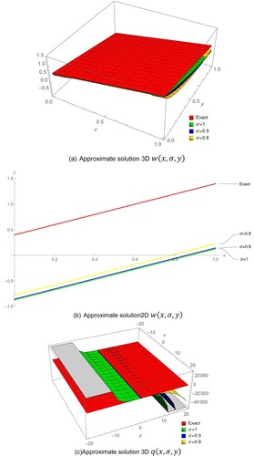
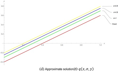
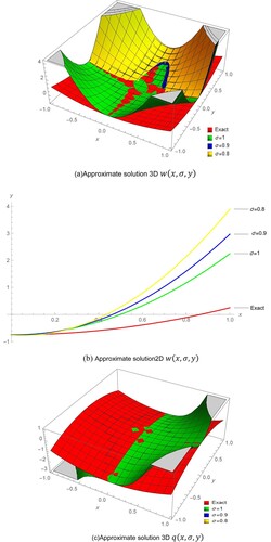
Figure 1. Comparison between Exact solution and approximate solution Example 1. (a) Approximate solution 3D $w\left(x,\sigma ,y\right)$. (b) Approximate solution2D $w\left(x,\sigma ,y\right)$. (c) Approximate solution 3D $q\left(x,\sigma ,y\right)$. (d) Approximate solution2D $q\left(x,\sigma ,y\right).$

The initial condition (9) $v\left(x,0\right)=g\left(x\right).$(9) On both sides, apply the Elzaki transform of Equation (8), we get [33] (10) $\begin{array}{rl}& E\left[J^{\alpha }w\left(x,y\right)\right]+E\left[Mw\left(x,y\right)\right]+E\left[Zw\left(x,y\right)\right]=E\left[q\left(x,y\right)\right],\\ & \frac{w\left(x,\delta \right)}{{\delta }^{\alpha }}-{\delta }^{2-\alpha }w\left(x,0\right)+E\left[Mw\left(x,y\right)\right]+E\left[Zw\left(x,y\right)\right]\\ & =E\left[q\left(x,y\right)\right],\\ & w\left(x,\delta \right)={\delta }^{2}w\left(x,0\right)-{\delta }^{\alpha }E\left[Mw\right(x,y)\\ & +Zw\left(x,y\right)+q\left(x,y\right)],\\ & w\left(x,\delta \right)={\delta }^{2}g\left(x\right)-{\delta }^{\alpha }E\left[Mw\left(x,y\right)+Zw\left(x,y\right)+q\left(x,y\right)\right].\end{array}$(10) The ADM is a method that $Zw\left(x,y\right)=\sum _{i=0}^{\mathrm{\infty }}{w}_i\left(x,y\right).$The problem’s nonlinear term is written as (11) $Zw\left(x,y\right)=\sum _{i=0}^{\mathrm{\infty }}{B}_i.$(11) Where (12) $B_i=\frac{1}{i!}{\left[\frac{d^i}{d{\gamma }^i}\left[Z\sum _{i=0}^{\mathrm{\infty }}\left({\gamma }^i{w}_i\right)\right]\right]}_{\gamma =0},i=0,1,2,\dots$(12) This say Adomain polynomials. (13) $\begin{array}{rl}E\left[\sum _{i=0}^{\mathrm{\infty }}w\left(x,\delta \right)\right]& ={\delta }^{2}g\left(x\right)-{\delta }^{\alpha }E[M\left(\sum _{i=0}^{\mathrm{\infty }}w\left(x,y\right)\right)\\ & +\sum _{i=0}^{\mathrm{\infty }}{B}_i+q\left(x,y\right)],\end{array}$(13) $\begin{array}{rl}w\left(x,y\right)& =g\left(x\right)-E^{-1}[{\delta }^{\alpha }E[M\left(\sum _{i=0}^{\mathrm{\infty }}w\left(x,y\right)\right)\\ & +\sum _{i=0}^{\mathrm{\infty }}{B}_i+q\left(x,y\right)]].\end{array}$ (14) $\begin{array}{rl}{w}_0\left(x,y\right)& =g\left(x\right),\end{array}$(14) (15) $\begin{array}{rl}{w}_{i+1}\left(x,y\right)& =-E^{-1}\left[{\delta }^{\alpha }E\left(Mw\left(x,y\right)\right)+B_i\right].\end{array}$(15)

4. Illustrative

Example 1

The fractional order of the system PDEs [42] (16) $\begin{array}{rl}& \frac{{\mathrm{\partial }}^{\alpha }w}{\mathrm{\partial }{y}^{\alpha }}-q\frac{\mathrm{\partial }w}{\mathrm{\partial }x}-\frac{\mathrm{\partial }q}{\mathrm{\partial }y}\frac{\mathrm{\partial }w}{\mathrm{\partial }\sigma }=1-x+\sigma +y,\end{array}$(16) (17) $\begin{array}{rl}& \frac{{\mathrm{\partial }}^{\alpha }q}{\mathrm{\partial }{y}^{\alpha }}-w\frac{\mathrm{\partial }q}{\mathrm{\partial }x}+\frac{\mathrm{\partial }w}{\mathrm{\partial }y}\frac{\mathrm{\partial }q}{\mathrm{\partial }\sigma }=1-x-\sigma -y,0<\alpha \le 1,\end{array}$(17) And initial condition (18) $\begin{array}{r}w\left(x,\sigma ,0\right)=x+\sigma -1,q\left(x,\sigma ,0\right)=x-\sigma +1.\end{array}$(18)

Taking the Elzaki of Equations (16) and (17), we have (19) $\begin{array}{rl}& E\left[\frac{{\mathrm{\partial }}^{\alpha }w}{\mathrm{\partial }{y}^{\alpha }}\right]=E\left[q\frac{\mathrm{\partial }w}{\mathrm{\partial }x}+\frac{\mathrm{\partial }q}{\mathrm{\partial }y}\frac{\mathrm{\partial }w}{\mathrm{\partial }\sigma }+1-x+\sigma +y\right],\end{array}$(19) (20) $\begin{array}{rl}& E\left[\frac{{\mathrm{\partial }}^{\alpha }q}{\mathrm{\partial }{y}^{\alpha }}\right]=E\left[w\frac{\mathrm{\partial }q}{\mathrm{\partial }x}-\frac{\mathrm{\partial }w}{\mathrm{\partial }y}\frac{\mathrm{\partial }q}{\mathrm{\partial }\sigma }+1-x-\sigma -y\right].\end{array}$(20) $\begin{array}{rl}& \frac{E\left[w\left(x,\sigma ,y\right)\right]}{{\delta }^{\alpha }}-{\delta }^2\left[w\left(x,\sigma ,y\right)\right]\\ & =E\left[q\frac{\mathrm{\partial }w}{\mathrm{\partial }x}+\frac{\mathrm{\partial }q}{\mathrm{\partial }x}\frac{\mathrm{\partial }w}{\mathrm{\partial }\sigma }+1-x+\sigma +y\right],\end{array}$ $\begin{array}{rl}& \frac{E\left[q\left(x,\sigma ,y\right)\right]}{{\delta }^{\alpha }}-{\delta }^2\left[q\left(x,\sigma ,y\right)\right]\\ & =E\left[w\frac{\mathrm{\partial }q}{\mathrm{\partial }x}-\frac{\mathrm{\partial }w}{\mathrm{\partial }y}\frac{\mathrm{\partial }q}{\mathrm{\partial }\sigma }+1-x-\sigma -y\right].\end{array}$Using the inverse transformation, we get $\begin{array}{rl}w\left(x,\sigma ,y\right)& =E^{-1}\left[{\delta }^{\alpha +2}w\right(x,\sigma ,y)+{\delta }^{\alpha }E[q\frac{\mathrm{\partial }w}{\mathrm{\partial }x}+\frac{\mathrm{\partial }q}{\mathrm{\partial }x}\frac{\mathrm{\partial }w}{\mathrm{\partial }\sigma }\\ & +1-x+\sigma +y]],\end{array}$ $\begin{array}{rl}q\left(x,\sigma ,y\right)& =E^{-1}\left[{\delta }^{\alpha +2}q\right(x,\sigma ,y)\\ & +{\delta }^{\alpha }E\left[w\frac{\mathrm{\partial }q}{\mathrm{\partial }x}-\frac{\mathrm{\partial }w}{\mathrm{\partial }y}\frac{\mathrm{\partial }q}{\mathrm{\partial }\sigma }+1-x-\sigma -y\right]].\end{array}$ (21) $\begin{array}{rl}w\left(x,\sigma ,y\right)& =x+\sigma -1+E^{-1}[{\delta }^{\alpha }E[q\frac{\mathrm{\partial }w}{\mathrm{\partial }x}+\frac{\mathrm{\partial }q}{\mathrm{\partial }x}\frac{\mathrm{\partial }w}{\mathrm{\partial }\sigma }\\ & +1-x+\sigma +y]],\end{array}$(21) (22) $\begin{array}{rl}q\left(x,\sigma ,y\right)& =x-\sigma +1+E^{-1}[{\delta }^{\alpha }E[q\frac{\mathrm{\partial }w}{\mathrm{\partial }x}+\frac{\mathrm{\partial }q}{\mathrm{\partial }x}\frac{\mathrm{\partial }w}{\mathrm{\partial }\sigma }\\ & +1-x+\sigma +y]].\end{array}$(22) We obtain the following results using the ADM technique. (23) $\begin{array}{rl}\sum _{i=0}^{\mathrm{\infty }}{w}_i\left(x,\sigma ,y\right)& =x+\sigma -1+E^{-1}[{\delta }^{\alpha }E[\sum _{i=0}^{\mathrm{\infty }}{B}_i(q,w)\\ & +\sum _{i=1}^{\mathrm{\infty }}{C}_i\left(q,w\right)+1-x+\sigma +y]],\end{array}$(23) (24) $\begin{array}{rl}\sum _{i=0}^{\mathrm{\infty }}{q}_i\left(x,\sigma ,y\right)& =x-\sigma +1+E^{-1}[{\delta }^{\alpha }E[\sum _{i=0}^{\mathrm{\infty }}{D}_i(w,q)\\ & +\sum _{i=1}^{\mathrm{\infty }}{F}_i\left(w,q\right)+1-x-\sigma -y]],\end{array}$(24) where Adomian polynomial components $B_i\left(q,w\right)$,$C_i\left(q,w\right),D_i\left(w,q\right),$ and $D_i\left(w,q\right)$ are given as follows: $B_0\left(q,w\right)=q_0\frac{\mathrm{\partial }{w}_0}{\mathrm{\partial }x},$ $B_1\left(q,w\right)=q_0\frac{\mathrm{\partial }{w}_1}{\mathrm{\partial }x}+q_1\frac{\mathrm{\partial }{w}_0}{\mathrm{\partial }x},$ (25) $B_2\left(q,w\right)=q_0\frac{\mathrm{\partial }{w}_2}{\mathrm{\partial }x}+q_1\frac{\mathrm{\partial }{w}_1}{\mathrm{\partial }x}+q_2\frac{\mathrm{\partial }{w}_0}{\mathrm{\partial }x},$(25) $C_0\left(q,w\right)=\frac{\mathrm{\partial }{q}_0}{\mathrm{\partial }y}\frac{\mathrm{\partial }{w}_0}{\mathrm{\partial }\sigma },$ $C_1\left(q,w\right)=\frac{\mathrm{\partial }{q}_0}{\mathrm{\partial }y}\frac{\mathrm{\partial }{w}_1}{\mathrm{\partial }\sigma }+\frac{\mathrm{\partial }{q}_1}{\mathrm{\partial }y}\frac{\mathrm{\partial }{w}_0}{\mathrm{\partial }\sigma },$ (26) $C_2\left(q,w\right)=\frac{\mathrm{\partial }{q}_0}{\mathrm{\partial }y}\frac{\mathrm{\partial }{w}_2}{\mathrm{\partial }\sigma }+\frac{\mathrm{\partial }{q}_1}{\mathrm{\partial }y}\frac{\mathrm{\partial }{w}_1}{\mathrm{\partial }\sigma }+\frac{\mathrm{\partial }{q}_2}{\mathrm{\partial }y}\frac{\mathrm{\partial }{w}_0}{\mathrm{\partial }\sigma },$(26) $D_0\left(w,q\right)=w_0\frac{\mathrm{\partial }{q}_0}{\mathrm{\partial }x},$ $D_1\left(w,q\right)=w_0\frac{\mathrm{\partial }{q}_1}{\mathrm{\partial }x}+w_1\frac{\mathrm{\partial }{q}_0}{\mathrm{\partial }x},$ (27) $D_2\left(w,q\right)=w_0\frac{\mathrm{\partial }{q}_2}{\mathrm{\partial }x}+w_1\frac{\mathrm{\partial }{q}_1}{\mathrm{\partial }x}+w_2\frac{\mathrm{\partial }{q}_0}{\mathrm{\partial }x},$(27) $F_0\left(w,q\right)=\frac{\mathrm{\partial }q{w}_0}{\mathrm{\partial }y}\frac{\mathrm{\partial }{q}_0}{\mathrm{\partial }\sigma },$ $F_1\left(w,q\right)=\frac{\mathrm{\partial }{w}_0}{\mathrm{\partial }y}\frac{\mathrm{\partial }{q}_1}{\mathrm{\partial }\sigma }+\frac{\mathrm{\partial }{w}_1}{\mathrm{\partial }y}\frac{\mathrm{\partial }{q}_0}{\mathrm{\partial }\sigma },$ (28) $\begin{array}{rl}& F_2\left(w,q\right)=\frac{\mathrm{\partial }{w}_0}{\mathrm{\partial }y}\frac{\mathrm{\partial }{q}_2}{\mathrm{\partial }\sigma }+\frac{\mathrm{\partial }{w}_1}{\mathrm{\partial }y}\frac{\mathrm{\partial }{q}_1}{\mathrm{\partial }\sigma }+\frac{\mathrm{\partial }{w}_2}{\mathrm{\partial }y}\frac{\mathrm{\partial }{q}_0}{\mathrm{\partial }\sigma },\end{array}$(28) (29) $\begin{array}{rl}& w_0\left(x,\sigma ,y\right)=x+\sigma -1,\end{array}$(29) (30) $\begin{array}{rl}& q_0\left(x,\sigma ,y\right)=x-\sigma +1.\end{array}$(30) (31) $\begin{array}{rl}& \sum _{i=0}^{\mathrm{\infty }}{w}_{i+1}\left(x,\sigma ,y\right)=E^{-1}[{\delta }^{\alpha }E[\sum _{i=0}^{\mathrm{\infty }}{B}_i(q,w)\\ & +\sum _{i=1}^{\mathrm{\infty }}{C}_i\left(q,w\right)+1-x+\sigma +y]],\end{array}$(31) (32) $\begin{array}{rl}& \sum _{i=0}^{\mathrm{\infty }}{q}_{i+1}\left(x,\sigma ,y\right)=E^{-1}[{\delta }^{\alpha }E[\sum _{i=0}^{\mathrm{\infty }}{D}_i(w,q)\\ & -\sum _{i=1}^{\mathrm{\infty }}{F}_i\left(w,q\right)+1-x-\sigma -y]],\end{array}$(32) For $i=0,1,2,\dots$ $\begin{array}{rl}{w}_1\left(x,\sigma ,y\right)& =E^{-1}[{\delta }^{\alpha }E[q_0\frac{\mathrm{\partial }{w}_0}{\mathrm{\partial }x}+\frac{\mathrm{\partial }{q}_0}{\mathrm{\partial }y}\frac{\mathrm{\partial }{w}_0}{\mathrm{\partial }x}\\ & +1-x+\sigma +y\phantom{\frac{\mathrm{\partial }{w}_0}{\mathrm{\partial }x}}]],\end{array}$ (33) $\begin{array}{rl}{w}_1\left(x,\sigma ,y\right)& =E^{-1}\left[2{\delta }^{\alpha +2}+{\delta }^{\alpha +3}\right]\\ & =\frac{2y^{\alpha }}{\mathrm{\Gamma }\left(\alpha +1\right)}+\frac{y^{\alpha +1}}{\mathrm{\Gamma }\left(\alpha +2\right)}.\end{array}$(33) $\begin{array}{rl}{q}_1& =E^{-1}[{\delta }^{\alpha }E[w_0\frac{\mathrm{\partial }{q}_0}{\mathrm{\partial }x}-\frac{\mathrm{\partial }{w}_0}{\mathrm{\partial }y}\frac{\mathrm{\partial }{q}_0}{\mathrm{\partial }\sigma }\\ & +1-x-\sigma -y]],\end{array}$ (34) $q_1=E^{-1}\left[-{\delta }^{\alpha +3}\right]=\frac{-y^{\alpha +1}}{\mathrm{\Gamma }\left(\alpha +2\right)}.$(34) The subsequent terms are $\begin{array}{rl}{w}_2\left(x,\sigma ,y\right)& =E^{-1}[{\delta }^{\alpha }E[q_0\frac{\mathrm{\partial }{w}_1}{\mathrm{\partial }x}+q_1\frac{\mathrm{\partial }{w}_0}{\mathrm{\partial }x}\\ & +\frac{\mathrm{\partial }{q}_0}{\mathrm{\partial }y}\frac{\mathrm{\partial }{w}_1}{\mathrm{\partial }\sigma }+\frac{\mathrm{\partial }{q}_1}{\mathrm{\partial }y}\frac{\mathrm{\partial }{w}_0}{\mathrm{\partial }\sigma }]]\\ & =\frac{-y^{2\alpha +1}}{\mathrm{\Gamma }\left(2\alpha +2\right)}-\frac{y^{2\alpha }}{\mathrm{\Gamma }\left(\alpha +2\right)},\\ q_2\left(x,\sigma ,y\right)& =E^{-1}[{\delta }^{\alpha }E[w_0\frac{\mathrm{\partial }{q}_1}{\mathrm{\partial }x}+w_1\frac{\mathrm{\partial }{q}_0}{\mathrm{\partial }x}-\frac{\mathrm{\partial }{w}_0}{\mathrm{\partial }y}\frac{\mathrm{\partial }{q}_1}{\mathrm{\partial }\sigma }\\ & -\frac{\mathrm{\partial }{w}_1}{\mathrm{\partial }y}\frac{\mathrm{\partial }{q}_0}{\mathrm{\partial }\sigma }]],\\ & =\left(\frac{2\mathrm{\Gamma }\left(\alpha +2\right)-\left(\alpha +1\right)\mathrm{\Gamma }\left(\alpha +1\right)}{\mathrm{\Gamma }\left(2\alpha +1\right)\mathrm{\Gamma }\left(\alpha +2\right)}\right)y^{2\alpha }\\ & +\frac{y^{2\alpha +1}}{\mathrm{\Gamma }\left(2\alpha +2\right)}-\frac{2\alpha \mathrm{\Gamma }\left(\alpha \right)y^{2\alpha -1}}{\mathrm{\Gamma }\left(\alpha +1\right)\mathrm{\Gamma }\left(2\alpha \right)},\end{array}$ $\begin{array}{rl}{w}_3\left(x,\sigma ,y\right)& =E^{-1}[{\delta }^{\alpha }E[q_0\frac{\mathrm{\partial }{w}_2}{\mathrm{\partial }x}+q_1\frac{\mathrm{\partial }{w}_1}{\mathrm{\partial }x}+q_2\frac{\mathrm{\partial }{w}_0}{\mathrm{\partial }x}\\ & +\frac{\mathrm{\partial }{q}_0}{\mathrm{\partial }y}\frac{\mathrm{\partial }{w}_2}{\mathrm{\partial }\sigma }+\frac{\mathrm{\partial }{q}_1}{\mathrm{\partial }y}\frac{\mathrm{\partial }{w}_1}{\mathrm{\partial }\sigma }+\frac{\mathrm{\partial }{q}_2}{\mathrm{\partial }y}\frac{\mathrm{\partial }{w}_0}{\mathrm{\partial }\sigma }]],\\ & =\frac{y^{3\alpha +1}}{\mathrm{\Gamma }\left(3\alpha +2\right)}\\ & +\left(\frac{2\mathrm{\Gamma }\left(\alpha +2\right)-\left(\alpha +1\right)\mathrm{\Gamma }\left(\alpha +1\right)}{\mathrm{\Gamma }\left(3\alpha +1\right)\mathrm{\Gamma }\left(\alpha +2\right)}\right)y^{3\alpha }\\ & +\frac{y^{3\alpha }}{\mathrm{\Gamma }\left(2\alpha +2\right)}\\ & -\frac{2\alpha \mathrm{\Gamma }\left(\alpha \right)y^{3\alpha -1}}{\mathrm{\Gamma }\left(\alpha +1\right)\mathrm{\Gamma }\left(3\alpha \right)}\\ & +\left(\frac{\begin{array}{c}\left(2\mathrm{\Gamma }\right(\alpha +2)-(\alpha +1)\\ \mathrm{\Gamma }\left(\alpha +1\right)\left)2\alpha \mathrm{\Gamma }\right(\alpha )\end{array}}{\mathrm{\Gamma }\left(3\alpha \right)\mathrm{\Gamma }\left(2\alpha +1\right)\mathrm{\Gamma }\left(\alpha +1\right)}\right)y^{3\alpha -1}\\ & -\left(\frac{2\alpha \mathrm{\Gamma }\left(\alpha \right)}{\mathrm{\Gamma }\left(2\alpha \right)\mathrm{\Gamma }\left(\alpha +1\right)}\right)y^{3\alpha -2},\end{array}$ $\begin{array}{rl}{q}_3\left(x,\sigma ,y\right)& =E^{-1}[{\delta }^{\alpha }E[w_0\frac{\mathrm{\partial }{q}_2}{\mathrm{\partial }x}+w_1\frac{\mathrm{\partial }{q}_1}{\mathrm{\partial }x}\\ & +w_2\frac{\mathrm{\partial }{q}_0}{\mathrm{\partial }x}-\frac{\mathrm{\partial }{w}_0}{\mathrm{\partial }y}\frac{\mathrm{\partial }{q}_2}{\mathrm{\partial }\sigma }\\ & -\frac{\mathrm{\partial }{w}_1}{\mathrm{\partial }y}\frac{\mathrm{\partial }{q}_1}{\mathrm{\partial }\sigma }-\frac{\mathrm{\partial }{w}_2}{\mathrm{\partial }y}\frac{\mathrm{\partial }{q}_0}{\mathrm{\partial }\sigma }]],\\ & =\frac{-y^{3\alpha +1}}{\mathrm{\Gamma }\left(3\alpha +2\right)}\\ & +\left(\frac{\left(\alpha +1\right)\mathrm{\Gamma }\left(\alpha +1\right)2\alpha \mathrm{\Gamma }\left(2\alpha \right)}{\mathrm{\Gamma }\left(3\alpha \right)\mathrm{\Gamma }\left(\alpha +2\right)\mathrm{\Gamma }\left(\alpha +2\right)}\right)y^{3\alpha -1},\end{array}$The EADM solution for Example 1 is $\begin{array}{rl}w\left(x,\sigma ,y\right)& =w_0\left(x,\sigma ,y\right)+w_1\left(x,\sigma ,y\right)+w_2\left(x,\sigma ,y\right)\\ & +w_3\left(x,\sigma ,y\right)+\dots \end{array}$ $\begin{array}{rl}q\left(x,\sigma ,y\right)& =q_0\left(x,\sigma ,y\right)+q_1\left(x,\sigma ,y\right)+q_2\left(x,\sigma ,y\right)\\ & +q_3\left(x,\sigma ,y\right)+\dots \end{array}$ (35) $\begin{array}{rl}w\left(x,\sigma ,y\right)& =x+\sigma -1+\frac{2y^{\alpha }}{\mathrm{\Gamma }\left(\alpha +1\right)}+\frac{y^{\alpha +1}}{\mathrm{\Gamma }\left(\alpha +2\right)}\\ & -\frac{y^{2\alpha +1}}{\mathrm{\Gamma }\left(2\alpha +2\right)}-\frac{y^{2\alpha }}{\mathrm{\Gamma }\left(2\alpha +1\right)}+\frac{y^{3\alpha +1}}{\mathrm{\Gamma }\left(3\alpha +2\right)}\\ & +\left(\frac{2\mathrm{\Gamma }\left(\alpha +2\right)-\left(\alpha +1\right)\mathrm{\Gamma }\left(\alpha +1\right)}{\mathrm{\Gamma }\left(3\alpha +1\right)\mathrm{\Gamma }\left(\alpha +2\right)}\right)y^{3\alpha }\\ & +\frac{y^{3\alpha }}{\mathrm{\Gamma }\left(2\alpha +2\right)}-\frac{2\alpha \mathrm{\Gamma }\left(\alpha \right){\text{y}}^{3\alpha -1}}{\mathrm{\Gamma }\left(\alpha +1\right)\mathrm{\Gamma }\left(3\alpha \right)}\\ & +\left(\frac{\begin{array}{c}\left(2\mathrm{\Gamma }\right(\alpha +2)-(\alpha +1)\\ \mathrm{\Gamma }\left(\alpha +1\right)\left)2\alpha \mathrm{\Gamma }\right(\alpha )\end{array}}{\mathrm{\Gamma }\left(3\alpha \right)\mathrm{\Gamma }\left(2\alpha +1\right)\mathrm{\Gamma }\left(\alpha +2\right)}\right)y^{3\alpha -1}\\ & -\left(\frac{2\alpha \mathrm{\Gamma }\left(\alpha \right)}{\mathrm{\Gamma }\left(2\alpha \right)\mathrm{\Gamma }\left(\alpha +1\right)}\right)y^{3\alpha -2}+\dots \end{array}$(35) (36) $\begin{array}{rl}q\left(x,\sigma ,y\right)& =x-\sigma +1-\frac{y^{\alpha +1}}{\mathrm{\Gamma }\left(\alpha +2\right)}\\ & +\left(\frac{2\mathrm{\Gamma }\left(\alpha +2\right)-\left(\alpha +1\right)\mathrm{\Gamma }\left(\alpha +1\right)}{\mathrm{\Gamma }\left(2\alpha +1\right)\mathrm{\Gamma }\left(\alpha +2\right)}\right)y^{2\alpha }\\ & +\frac{y^{2\alpha +1}}{\mathrm{\Gamma }\left(2\alpha +2\right)}-\frac{2\alpha \mathrm{\Gamma }\left(\alpha \right)y^{2\alpha -1}}{\mathrm{\Gamma }\left(\alpha +1\right)\mathrm{\Gamma }\left(2\alpha \right)}\\ & -\frac{y^{3\alpha +1}}{\mathrm{\Gamma }\left(3\alpha +2\right)}\\ & +\left(\frac{\left(\alpha +1\right)\mathrm{\Gamma }\left(\alpha +1\right)2\alpha \mathrm{\Gamma }\left(2\alpha \right)}{\mathrm{\Gamma }\left(3\alpha \right)\mathrm{\Gamma }\left(\alpha +2\right)\mathrm{\Gamma }\left(\alpha +2\right)}\right)y^{3\alpha -1}+\dots \end{array}$(36) When $\alpha =1,$ then EADM solution is (Figure 1) (37) $\begin{array}{rl}w\left(x,\sigma ,y\right)& =x+\sigma +y-1,\end{array}$(37) (38) $\begin{array}{rl}q\left(x,\sigma ,y\right)& =x-\sigma -y+1.\end{array}$(38)

Example 2

The fractional order PDEs system in [42] (39) $\begin{array}{rl}& \frac{{\mathrm{\partial }}^{\alpha }w}{\mathrm{\partial }{x}^{\alpha }}-q\frac{\mathrm{\partial }w}{\mathrm{\partial }y}+w\frac{\mathrm{\partial }q}{\mathrm{\partial }y}=-1+e^x\sin y,\end{array}$(39) (40) $\begin{array}{rl}& \frac{{\mathrm{\partial }}^{\alpha }q}{\mathrm{\partial }{x}^{\alpha }}+\frac{\mathrm{\partial }w}{\mathrm{\partial }y}\frac{\mathrm{\partial }q}{\mathrm{\partial }x}-\frac{\mathrm{\partial }q}{\mathrm{\partial }y}\frac{\mathrm{\partial }w}{\mathrm{\partial }x}=-1-e^{-x}\cos \text{y},0<\alpha \le 1,\end{array}$(40) With the initial conditions (41) $\begin{array}{r}w\left(0,y\right)=\sin y,q\left(0,y\right)=\cos y.\end{array}$(41)

By using Elzaki transform of (4.24) and (4.25) we have $E\left[\frac{{\mathrm{\partial }}^{\alpha }w}{\mathrm{\partial }{x}^{\alpha }}\right]=E\left[q\frac{\mathrm{\partial }w}{\mathrm{\partial }y}-w\frac{\mathrm{\partial }q}{\mathrm{\partial }y}-1+e^x\sin y\right],$ $E\left[\frac{{\mathrm{\partial }}^{\alpha }q}{\mathrm{\partial }{x}^{\alpha }}\right]=E\left[-\frac{\mathrm{\partial }w}{\mathrm{\partial }y}\frac{\mathrm{\partial }q}{\mathrm{\partial }x}-\frac{\mathrm{\partial }q}{\mathrm{\partial }y}\frac{\mathrm{\partial }w}{\mathrm{\partial }x}-1-e^{-x}\cos y\right],$ $\begin{array}{rl}& \frac{E\left[w\left(x,y\right)\right]}{{\delta }^{\alpha }}-{\delta }^2\left[w\left(0,y\right)\right]\\ & =E\left[q\frac{\mathrm{\partial }w}{\mathrm{\partial }y}-w\frac{\mathrm{\partial }q}{\mathrm{\partial }y}-1+e^x\sin y\right],\end{array}$ $\begin{array}{rl}& \frac{E\left[q\left(x,y\right)\right]}{{\delta }^{\alpha }}-{\delta }^2\left[q\left(0,y\right)\right]\\ & =E\left[-\frac{\mathrm{\partial }w}{\mathrm{\partial }y}\frac{\mathrm{\partial }q}{\mathrm{\partial }x}-\frac{\mathrm{\partial }q}{\mathrm{\partial }y}\frac{\mathrm{\partial }w}{\mathrm{\partial }x}-1-e^{-x}\cos y\right],\end{array}$We get the result by applying the inverse transformation. (42) $\begin{array}{rl}w\left(x,y\right)& =E^{-1}\left[{\delta }^{\alpha +2}w\right(0,y)\\ & +{\delta }^{\alpha }E\left[q\frac{\mathrm{\partial }w}{\mathrm{\partial }y}-w\frac{\mathrm{\partial }q}{\mathrm{\partial }y}-1+e^x\sin y\right]],\end{array}$(42) (43) $\begin{array}{rl}q\left(x,y\right)& =E^{-1}\left[{\delta }^{\alpha +2}q\right(0,y)+{\delta }^{\alpha }E[-\frac{\mathrm{\partial }w}{\mathrm{\partial }y}\frac{\mathrm{\partial }q}{\mathrm{\partial }x}\\ & -\frac{\mathrm{\partial }q}{\mathrm{\partial }y}\frac{\mathrm{\partial }w}{\mathrm{\partial }x}-1-e^{-x}\cos y]],\end{array}$(43) Using the ADM procedure, we have (44) $\begin{array}{rl}{w}_0\left(x,y\right)& =E^{-1}\left[{\delta }^{\alpha +2}w\left(0,y\right)\right]=E^{-1}\left[{\delta }^{\alpha +2}\sin y\right]=\sin y,\end{array}$(44) (45) $\begin{array}{rl}{q}_0\left(x,y\right)& =E^{-1}\left[{\delta }^{\alpha +2}q\left(0,y\right)\right]\\ & =E^{-1}\left[{\delta }^{\alpha +2}\cos y\right]=\cos y,\end{array}$(45) (46) $\begin{array}{rl}{w}_{i+1}\left(x,y\right)& =E^{-1}[{\delta }^{\alpha }E[q_i\frac{\mathrm{\partial }{w}_i}{\mathrm{\partial }y}-w_i\frac{\mathrm{\partial }{q}_i}{\mathrm{\partial }y}\\ & -1+e^x\sin y]].\end{array}$(46) (47) $\begin{array}{rl}{q}_{i+1}& =E^{-1}[{\delta }^{\alpha }E[-\frac{\mathrm{\partial }{w}_i}{\mathrm{\partial }y}\frac{\mathrm{\partial }{q}_i}{\mathrm{\partial }x}-\frac{\mathrm{\partial }{q}_i}{\mathrm{\partial }y}\frac{\mathrm{\partial }{w}_i}{\mathrm{\partial }x}\\ & -1-e^{-x}\cos y]],\end{array}$(47) $i=0,1,2,\dots$ $\text{for}i=0$ $\begin{array}{rl}{w}_1\left(x,y\right)& =E^{-1}[{\delta }^{\alpha }E[q_0\frac{\mathrm{\partial }{w}_0}{\mathrm{\partial }y}-w_0\frac{\mathrm{\partial }{q}_0}{\mathrm{\partial }y}\\ & -1+e^x\sin y\phantom{\frac{\mathrm{\partial }{q}_0}{\mathrm{\partial }y}}]],\end{array}$ $\begin{array}{rl}{w}_1\left(x,y\right)& =E^{-1}\left[\frac{\sin y{\delta }^{\alpha +2}}{1-\delta }\right]\\ & =\sin y{x}^{\alpha }\sum _{m=0}^{\mathrm{\infty }}\frac{x^m}{\mathrm{\Gamma }\left(m+\alpha +1\right)}\end{array}$ $\begin{array}{rl}{q}_1\left(x,y\right)& =E^{-1}[{\delta }^{\alpha }E[-\frac{\mathrm{\partial }{w}_0}{\mathrm{\partial }y}\frac{\mathrm{\partial }{q}_0}{\mathrm{\partial }x}-\frac{\mathrm{\partial }{q}_0}{\mathrm{\partial }y}\frac{\mathrm{\partial }{w}_0}{\mathrm{\partial }x}\\ & -1-e^{-x}\cos y\phantom{\frac{\mathrm{\partial }{q}_0}{\mathrm{\partial }y}}]],\end{array}$ $\begin{array}{rl}{q}_1\left(x,y\right)& =E^{-1}\left[-{\delta }^{\alpha +2}-\cos y\frac{{\delta }^{\alpha +2}}{1+\delta }\right]\\ & =\frac{y^{\alpha }}{\mathrm{\Gamma }\left(\alpha +1\right)}-\cos y{x}^{\alpha }\sum _{m=0}^{\mathrm{\infty }}\frac{-x^m}{\mathrm{\Gamma }\left(m+\alpha +1\right)},\end{array}$ $\begin{array}{rl}{w}_2\left(x,y\right)& =E^{-1}[{\delta }^{\alpha }E[q_0\frac{\mathrm{\partial }{w}_1}{\mathrm{\partial }y}+q_1\frac{\mathrm{\partial }{w}_0}{\mathrm{\partial }y}\\ & -w_0\frac{\mathrm{\partial }{q}_1}{\mathrm{\partial }y}-w_1\frac{\mathrm{\partial }{q}_0}{\mathrm{\partial }y}]]\\ & =\sum _{m=1}^{\mathrm{\infty }}\frac{x^{2\alpha +m}}{\mathrm{\Gamma }\left(2\alpha +m+1\right)}-\sum _{m=0}^{\mathrm{\infty }}\frac{{\left(-x\right)}^{2\alpha +m}}{\mathrm{\Gamma }\left(2\alpha +m+1\right)}\\ & -\cos y\frac{x^{2\alpha }}{\mathrm{\Gamma }\left(2\alpha +1\right)},\end{array}$ $\begin{array}{rl}{q}_2\left(x,y\right)& =E^{-1}[{\delta }^{\alpha }E[-\frac{\mathrm{\partial }{w}_0}{\mathrm{\partial }y}\frac{\mathrm{\partial }{q}_1}{\mathrm{\partial }x}-\frac{\mathrm{\partial }{w}_1}{\mathrm{\partial }y}\frac{\mathrm{\partial }{q}_0}{\mathrm{\partial }x}\\ & -\frac{\mathrm{\partial }{q}_0}{\mathrm{\partial }y}\frac{\mathrm{\partial }{w}_1}{\mathrm{\partial }x}-\frac{\mathrm{\partial }{q}_1}{\mathrm{\partial }y}\frac{\mathrm{\partial }{w}_0}{\mathrm{\partial }x}]],\\ & =\cos y\frac{x^{2\alpha -1}}{\mathrm{\Gamma }\left(2\alpha \right)}+{\cos }^{2}y\sum _{m=0}^{\mathrm{\infty }}\frac{{\left(-x\right)}^{2\alpha +m-1}}{\mathrm{\Gamma }\left(2\alpha +m\right)}\\ & -{\sin }^{2}y\sum _{m=0}^{\mathrm{\infty }}\frac{x^{2\alpha +m-1}}{\mathrm{\Gamma }\left(2\alpha +m\right)}.\end{array}$For example 2, the following is the outcome: $\begin{array}{rl}w\left(x,y\right)& =w_0\left(x,y\right)+w_1\left(x,y\right)+w_2\left(x,y\right)\\ & +w_3\left(x,y\right)+\dots \end{array}$ $q\left(x,y\right)=q_0\left(x,y\right)+q_1\left(x,y\right)+q_2\left(x,y\right)+q_3\left(x,y\right)+\dots$ (48) $\begin{array}{rl}w\left(x,y\right)& =\sin y+\sin y{x}^{\alpha }\sum _{m=0}^{\mathrm{\infty }}\frac{x^m}{\mathrm{\Gamma }\left(m+\alpha +1\right)}\\ & +\sum _{m=0}^{\mathrm{\infty }}\frac{x^{2\alpha +m}}{\mathrm{\Gamma }\left(2\alpha +m+1\right)}\\ & -\sum _{m=0}^{\mathrm{\infty }}\frac{{\left(-x\right)}^{2\alpha +m}}{\mathrm{\Gamma }\left(2\alpha +m+1\right)}-\cos y\frac{x^{2\alpha }}{\mathrm{\Gamma }\left(2\alpha +1\right)}\dots \end{array}$(48) (49) $\begin{array}{rl}q\left(x,y\right)& =\cos y-\frac{y^{\alpha }}{\mathrm{\Gamma }\left(\alpha +1\right)}\\ & -\cos y{x}^{\alpha }\sum _{m=0}^{\mathrm{\infty }}\frac{-x^m}{\mathrm{\Gamma }\left(m+\alpha +1\right)}+\cos y\frac{x^{2\alpha -1}}{\mathrm{\Gamma }\left(2\alpha \right)}\\ & +{\cos }^{2}y\sum _{m=0}^{\mathrm{\infty }}\frac{{\left(-x\right)}^{2\alpha +m-1}}{\mathrm{\Gamma }\left(2\alpha +m\right)}\\ & +{\sin }^{2}y\sum _{m=0}^{\mathrm{\infty }}\frac{x^{2\alpha +m-1}}{\mathrm{\Gamma }\left(2\alpha +m\right)}+\dots \end{array}$(49) When $\alpha =1$, then LADM solution is (Figure 2) (50) $\begin{array}{rl}w\left(x,y\right)& =e^x\sin y,\end{array}$(50) (51) $\begin{array}{rl}q\left(x,y\right)& =e^{-x}\cos y.\end{array}$(51)

Example 3

the system of inhomogeneous fractional-order nonlinear PDEs in [42] (52) $\begin{array}{rl}& \frac{{\mathrm{\partial }}^{\alpha }w}{\mathrm{\partial }{y}^{\alpha }}-\frac{\mathrm{\partial }v}{\mathrm{\partial }x}\frac{\mathrm{\partial }q}{\mathrm{\partial }y}-\frac{1}{2}\frac{\mathrm{\partial }v}{\mathrm{\partial }y}\frac{{\mathrm{\partial }}^{2}w}{\mathrm{\partial }{x}^2}=-4xy,\end{array}$(52) (53) $\begin{array}{rl}& \frac{{\mathrm{\partial }}^{\alpha }q}{\mathrm{\partial }{y}^{\alpha }}-\frac{\mathrm{\partial }v}{\mathrm{\partial }y}\frac{{\mathrm{\partial }}^{2}q}{\mathrm{\partial }{x}^2}=6y,\end{array}$(53) (54) $\begin{array}{rl}& \frac{{\mathrm{\partial }}^{\alpha }v}{\mathrm{\partial }{y}^{\alpha }}-\frac{{\mathrm{\partial }}^{2}w}{\mathrm{\partial }{x}^2}-\frac{\mathrm{\partial }q}{\mathrm{\partial }x}\frac{\mathrm{\partial }v}{\mathrm{\partial }y}=4x-2y-2,0<\alpha \le 1.\end{array}$(54)

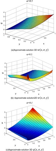
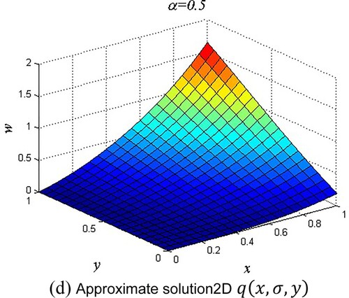
Figure 2. Comparison between Exact solution and approximate solution Example 2. (a) Approximate solution 3D $w\left(x,\sigma ,y\right)$. (b) Approximate solution2D $w\left(x,\sigma ,y\right)$. (c)Approximate solution 3D $q\left(x,\sigma ,y\right)$. (d) Approximate solution2D $q\left(x,\sigma ,y\right).$

With the initial conditions (55) $w\left(x,0\right)=x^2+1,q\left(x,0\right)=x^2-1,v\left(x,0\right)=x^2-1.$(55) Using the Elzaki transform of (4.37), (4.38) and (4.39) we get (56) $\begin{array}{rl}& E\left[\frac{{\mathrm{\partial }}^{\alpha }w}{\mathrm{\partial }{y}^{\alpha }}\right]=E\left[\frac{\mathrm{\partial }v}{\mathrm{\partial }x}\frac{\mathrm{\partial }q}{\mathrm{\partial }y}+\frac{1}{2}\frac{\mathrm{\partial }v}{\mathrm{\partial }y}\frac{{\mathrm{\partial }}^{2}w}{\mathrm{\partial }{x}^2}-4xy\right],\end{array}$(56) (57) $\begin{array}{rl}& E\left[\frac{{\mathrm{\partial }}^{\alpha }q}{\mathrm{\partial }{y}^{\alpha }}\right]=E\left[\frac{\mathrm{\partial }v}{\mathrm{\partial }y}\frac{{\mathrm{\partial }}^{2}w}{\mathrm{\partial }{x}^2}+6y\right],\end{array}$(57) (58) $\begin{array}{rl}& E\left[\frac{{\mathrm{\partial }}^{\alpha }v}{\mathrm{\partial }{y}^{\alpha }}\right]=E\left[\frac{{\mathrm{\partial }}^{2}w}{\mathrm{\partial }{x}^2}+\frac{\mathrm{\partial }q}{\mathrm{\partial }x}\frac{\mathrm{\partial }v}{\mathrm{\partial }y}+4xy-2y-2\right],\end{array}$(58) $\begin{array}{rl}& \frac{E\left[w\left(x,y\right)\right]}{{\delta }^{\alpha }}-{\delta }^2\left[w\left(x,0\right)\right]\\ & =E\left[\frac{\mathrm{\partial }v}{\mathrm{\partial }x}\frac{\mathrm{\partial }q}{\mathrm{\partial }y}+\frac{1}{2}\frac{\mathrm{\partial }v}{\mathrm{\partial }y}\frac{{\mathrm{\partial }}^{2}w}{\mathrm{\partial }{x}^2}-4xy\right],\end{array}$ $\frac{E\left[q\left(x,y\right)\right]}{{\delta }^{\alpha }}-{\delta }^2\left[q\left(x,0\right)\right]=E\left[\frac{\mathrm{\partial }v}{\mathrm{\partial }y}\frac{{\mathrm{\partial }}^{2}w}{\mathrm{\partial }{x}^2}+6y\right],$ $\begin{array}{rl}& \frac{E\left[v\left(x,y\right)\right]}{{\delta }^{\alpha }}-{\delta }^2\left[v\left(x,0\right)\right]\\ & =E\left[\frac{\mathrm{\partial }v}{\mathrm{\partial }x}\frac{\mathrm{\partial }q}{\mathrm{\partial }y}+\frac{1}{2}\frac{\mathrm{\partial }v}{\mathrm{\partial }y}\frac{{\mathrm{\partial }}^{2}w}{\mathrm{\partial }{x}^2}-4xy\right],\end{array}$We get the result by applying the inverse transformation. (59) $\begin{array}{rl}w\left(x,y\right)& =E^{-1}\left[{\delta }^{\alpha +2}w\right(x,0)+{\delta }^{\alpha }E[\frac{\mathrm{\partial }v}{\mathrm{\partial }x}\frac{\mathrm{\partial }q}{\mathrm{\partial }y}\\ & +\frac{1}{2}\frac{\mathrm{\partial }v}{\mathrm{\partial }y}\frac{{\mathrm{\partial }}^{2}w}{\mathrm{\partial }{x}^2}-4xy]],\end{array}$(59) (60) $\begin{array}{rl}q\left(x,y\right)& =E^{-1}\left[{\delta }^{\alpha +2}q\left(x,0\right)+{\delta }^{\alpha }E\left[\frac{\mathrm{\partial }v}{\mathrm{\partial }y}\frac{{\mathrm{\partial }}^{2}w}{\mathrm{\partial }{x}^2}+6y\right]\right],\end{array}$(60) (61) $\begin{array}{rl}v\left(x,y\right)& =E^{-1}\left[{\delta }^{\alpha +2}v\right(x,0)\\ & +{\delta }^{\alpha }E\left[\frac{{\mathrm{\partial }}^{2}w}{\mathrm{\partial }{x}^2}+\frac{\mathrm{\partial }q}{\mathrm{\partial }x}\frac{\mathrm{\partial }v}{\mathrm{\partial }y}+4xy-2y-2\right]].\end{array}$(61) Using the ADM procedure, we have $\begin{array}{rl}{w}_0\left(x,y\right)& =E^{-1}\left[{\delta }^{\alpha +2}w\left(x,0\right)\right]\\ & =E^{-1}\left[{\delta }^{\alpha +2}{x}^2+1\right]=x^2+1,\end{array}$ $\begin{array}{rl}{q}_0\left(x,y\right)& =E^{-1}\left[{\delta }^{\alpha +2}q\left(x,0\right)\right]\\ & =E^{-1}\left[{\delta }^{\alpha +2}{x}^2-1\right]=x^2-1,\end{array}$ $\begin{array}{rl}{v}_0\left(x,y\right)& =E^{-1}\left[{\delta }^{\alpha +2}v\left(x,0\right)\right]\\ & =E^{-1}\left[{\delta }^{\alpha +2}{x}^2-1\right]=x^2-1,\end{array}$ (62) $w_{i+1}\left(x,y\right)=E^{-1}\left[{\delta }^{\alpha }E\left[\frac{\mathrm{\partial }v}{\mathrm{\partial }x}\frac{\mathrm{\partial }q}{\mathrm{\partial }y}+\frac{1}{2}\frac{\mathrm{\partial }v}{\mathrm{\partial }y}\frac{{\mathrm{\partial }}^{2}w}{\mathrm{\partial }{x}^2}-4xy\right]\right],$(62) (63) $q_{i+1}\left(\text{x},\text{y}\right)=E^{-1}\left[{\delta }^{\alpha }E\left[\frac{\mathrm{\partial }v}{\mathrm{\partial }y}\frac{{\mathrm{\partial }}^{2}w}{\mathrm{\partial }{x}^2}+6y\right]\right],$(63) (64) $\begin{array}{rl}& {\text{v}}_{\text{i}+1}\left(\text{x},\text{y}\right)\\ & ={\text{E}}^{-1}\left[{\delta }^{\alpha }\text{E}\left[\frac{{\mathrm{\partial }}^2\text{w}}{\mathrm{\partial }{\text{x}}^2}+\frac{\mathrm{\partial }\text{q}}{\mathrm{\partial }\text{x}}\frac{\mathrm{\partial }\text{v}}{\mathrm{\partial }\text{y}}+4\text{xy}-2\text{y}-2\right]\right],\end{array}$(64) $i=0,1,2,\dots$ $\text{for}i=0$ $\begin{array}{r}{w}_1\left(x,y\right)=E^{-1}\left[{\delta }^{\alpha }E\left[\frac{\mathrm{\partial }{v}_0}{\mathrm{\partial }x}\frac{\mathrm{\partial }{q}_0}{\mathrm{\partial }y}+\frac{1}{2}\frac{\mathrm{\partial }{v}_0}{\mathrm{\partial }y}\frac{{\mathrm{\partial }}^2{w}_0}{\mathrm{\partial }{x}^2}-4xy\right]\right],\end{array}$ $\begin{array}{r}{w}_1\left(x,y\right)=E^{-1}\left[-4x{\delta }^{\alpha +3}\right]=\frac{-4x{y}^{\alpha +1}}{\mathrm{\Gamma }\left(\alpha +2\right)},\end{array}$ $\begin{array}{r}{q}_1\left(x,y\right)=E^{-1}\left[{\delta }^{\alpha }E\left[\frac{\mathrm{\partial }{v}_0}{\mathrm{\partial }y}\frac{{\mathrm{\partial }}^2{w}_0}{\mathrm{\partial }{x}^2}+6y\right]\right],\end{array}$ $\begin{array}{r}{q}_1\left(x,y\right)=E^{-1}\left[6{\delta }^{\alpha +3}\right]=\frac{6y^{\alpha +1}}{\mathrm{\Gamma }\left(\alpha +2\right)},\end{array}$ $\begin{array}{rl}{v}_1\left(x,y\right)& =E^{-1}[{\delta }^{\alpha }E[\frac{{\mathrm{\partial }}^2{w}_0}{\mathrm{\partial }{x}^2}+\frac{\mathrm{\partial }{q}_0}{\mathrm{\partial }x}\frac{\mathrm{\partial }{v}_0}{\mathrm{\partial }y}\\ & +4xy-2y-2\phantom{\frac{\mathrm{\partial }{q}_0}{\mathrm{\partial }y}}]],\end{array}$ $\begin{array}{rl}{v}_1\left(x,y\right)& =E^{-1}\left[4x{\delta }^{\alpha +3}-2{\delta }^{\alpha +3}\right]\\ & =\frac{4x{y}^{\alpha +1}}{\mathrm{\Gamma }\left(\alpha +2\right)}-\frac{2y^{\alpha +1}}{\mathrm{\Gamma }\left(\alpha +2\right)},\end{array}$The words that follow are: $\begin{array}{rl}{w}_2\left(x,y\right)& =E^{-1}[{\delta }^{\alpha }E[\frac{\mathrm{\partial }{v}_0}{\mathrm{\partial }x}\frac{\mathrm{\partial }{q}_1}{\mathrm{\partial }y}+\frac{\mathrm{\partial }{v}_1}{\mathrm{\partial }x}\frac{\mathrm{\partial }{q}_0}{\mathrm{\partial }y}+\frac{1}{2}\frac{\mathrm{\partial }{v}_0}{\mathrm{\partial }y}\frac{{\mathrm{\partial }}^2{w}_1}{\mathrm{\partial }{x}^2}\\ & +\frac{1}{2}\frac{\mathrm{\partial }{v}_1}{\mathrm{\partial }y}\frac{{\mathrm{\partial }}^2{w}_0}{\mathrm{\partial }{x}^2}]],\\ & =\frac{16x{y}^{2\alpha }}{\mathrm{\Gamma }\left(\alpha +2\right)}-\frac{2y^{\alpha }}{\mathrm{\Gamma }\left(\alpha +2\right)}\end{array}$ $\begin{array}{rl}{q}_2\left(x,y\right)& =E^{-1}\left[{\delta }^{\alpha }E\left[\frac{\mathrm{\partial }{v}_0}{\mathrm{\partial }x}\frac{{\mathrm{\partial }}^2{w}_1}{\mathrm{\partial }{x}^2}+\frac{1}{2}\frac{\mathrm{\partial }{v}_1}{\mathrm{\partial }y}\frac{{\mathrm{\partial }}^2{w}_0}{\mathrm{\partial }{x}^2}\right]\right],\\ & =\frac{8x{y}^{2\alpha }}{\mathrm{\Gamma }\left(\alpha +2\right)}-\frac{4y^{2\alpha }}{\mathrm{\Gamma }\left(\alpha +2\right)}\end{array}$ $\begin{array}{rl}{v}_2\left(x,y\right)& =E^{-1}\left[{\delta }^{\alpha }E\left[\frac{{\mathrm{\partial }}^2{w}_1}{\mathrm{\partial }{x}^2}+\frac{\mathrm{\partial }{q}_0}{\mathrm{\partial }x}\frac{\mathrm{\partial }{v}_1}{\mathrm{\partial }y}+\frac{\mathrm{\partial }{q}_1}{\mathrm{\partial }x}\frac{\mathrm{\partial }{v}_0}{\mathrm{\partial }y}\right]\right],\\ & =\frac{8x^2{y}^{2\alpha }}{\mathrm{\Gamma }\left(\alpha +2\right)}-\frac{4x{y}^{2\alpha }}{\mathrm{\Gamma }\left(\alpha +2\right)}\end{array}$ $\begin{array}{rl}{w}_3\left(x,y\right)& =E^{-1}\left[{\delta }^{\alpha }E\left[\frac{\mathrm{\partial }{v}_0}{\mathrm{\partial }x}\frac{\mathrm{\partial }{q}_2}{\mathrm{\partial }y}+\frac{\mathrm{\partial }{v}_1}{\mathrm{\partial }x}\frac{\mathrm{\partial }{q}_1}{\mathrm{\partial }y}+\frac{\mathrm{\partial }{v}_2}{\mathrm{\partial }x}\frac{\mathrm{\partial }{q}_0}{\mathrm{\partial }y}\right]\right],\\ & =E^{-1}[{\delta }^{\alpha }E[\frac{1}{2}\frac{\mathrm{\partial }{v}_0}{\mathrm{\partial }x}\frac{{\mathrm{\partial }}^2{w}_2}{\mathrm{\partial }{x}^2}+\frac{1}{2}\frac{\mathrm{\partial }{v}_1}{\mathrm{\partial }x}\frac{{\mathrm{\partial }}^2{w}_1}{\mathrm{\partial }{x}^2}\\ & +\frac{1}{2}\frac{\mathrm{\partial }{v}_2}{\mathrm{\partial }x}\frac{{\mathrm{\partial }}^2{w}_0}{\mathrm{\partial }{x}^2}]],\\ & =\left(\frac{4\left(\alpha +1\right)\mathrm{\Gamma }\left(2\alpha +2\right)}{\mathrm{\Gamma }\left(\alpha +2\right)\mathrm{\Gamma }\left(\alpha +2\right)\mathrm{\Gamma }\left(3\alpha +2\right)}\right)y^{3\alpha +1}\\ & +\left(\frac{48x^2\left(\alpha \right)\mathrm{\Gamma }\left(2\alpha \right)}{\mathrm{\Gamma }\left(\alpha +2\right)\mathrm{\Gamma }\left(3\alpha \right)}\right)y^{3\alpha -1}\\ & -\left(\frac{24x\left(\alpha \right)\mathrm{\Gamma }\left(2\alpha \right)}{\mathrm{\Gamma }\left(\alpha +2\right)\mathrm{\Gamma }\left(3\alpha \right)}\right)y^{3\alpha -1},\end{array}$ $\begin{array}{rl}{q}_3\left(x,y\right)& =E^{-1}[{\delta }^{\alpha }E[\frac{\mathrm{\partial }{v}_0}{\mathrm{\partial }x}\frac{{\mathrm{\partial }}^2{w}_2}{\mathrm{\partial }{x}^2}+\frac{\mathrm{\partial }{v}_1}{\mathrm{\partial }x}\frac{{\mathrm{\partial }}^2{w}_1}{\mathrm{\partial }{x}^2}\\ & +\frac{\mathrm{\partial }{v}_2}{\mathrm{\partial }x}\frac{{\mathrm{\partial }}^2{w}_0}{\mathrm{\partial }{x}^2}]],\\ & =\left(\frac{32x^2\alpha \mathrm{\Gamma }\left(2\alpha \right)}{\mathrm{\Gamma }\left(\alpha +2\right)\mathrm{\Gamma }\left(3\alpha \right)}\right)y^{3\alpha -1}\\ & -\left(\frac{16x\alpha \mathrm{\Gamma }\left(2\alpha \right)}{\mathrm{\Gamma }\left(\alpha +2\right)\mathrm{\Gamma }\left(3\alpha \right)}\right)y^{3\alpha -1},\end{array}$ $\begin{array}{rl}{v}_3\left(x,y\right)& =E^{-1}[{\delta }^{\alpha }E[\frac{{\mathrm{\partial }}^2{w}_2}{\mathrm{\partial }{x}^2}+\frac{\mathrm{\partial }{q}_0}{\mathrm{\partial }x}\frac{\mathrm{\partial }{v}_2}{\mathrm{\partial }y}\\ & +\frac{\mathrm{\partial }{q}_1}{\mathrm{\partial }x}\frac{\mathrm{\partial }{v}_1}{\mathrm{\partial }y}+\frac{\mathrm{\partial }{q}_2}{\mathrm{\partial }x}\frac{\mathrm{\partial }{v}_0}{\mathrm{\partial }y}]],\\ & =\left(\frac{32x^3\alpha \mathrm{\Gamma }\left(2\alpha \right)}{\mathrm{\Gamma }\left(\alpha +2\right)\mathrm{\Gamma }\left(3\alpha \right)}\right)y^{3\alpha -1}\\ & -\left(\frac{16x^2\alpha \mathrm{\Gamma }\left(2\alpha \right)}{\mathrm{\Gamma }\left(\alpha +2\right)\mathrm{\Gamma }\left(3\alpha \right)}\right)y^{3\alpha -1}.\end{array}$The obtained result for example 3 $\begin{array}{rl}w\left(x,y\right)& =w_0\left(x,y\right)+w_1\left(x,y\right)+w_2\left(x,y\right)\\ & +w_3\left(x,y\right)+\dots \end{array}$ $q\left(x,y\right)=q_0\left(x,y\right)+q_1\left(x,y\right)+q_2\left(x,y\right)+q_3\left(x,y\right)+\dots$ $v\left(x,y\right)=v_0\left(x,y\right)+v_1\left(x,y\right)+v_2\left(x,y\right)+v_3\left(x,y\right)+\dots$ (65) $\begin{array}{rl}w\left(x,y\right)& =x^2+1-\frac{4x{y}^{\alpha +1}}{\text{Gamma}\left[\alpha +2\right]}+\frac{16x{y}^{2\alpha }}{\text{Gamma}\left[\alpha +2\right]}\\ & -\frac{2y^{\alpha }}{\text{Gamma}\left[\alpha +2\right]}\\ & +\left(\frac{4\left(\alpha +1\right)\mathrm{\Gamma }\left(2\alpha +2\right)}{\begin{array}{c}\text{Gamma}\left[\alpha +2\right]\text{Gamma}\left[\alpha +2\right]\\ \text{Gamma}\left[3\alpha +2\right]\end{array}}\right)y^{3\alpha +1}\\ & +\left(\frac{48x^2\left(\alpha \right)\text{Gamma}\left[2\alpha \right]}{\text{Gamma}\left[\alpha +2\right]\text{Gamma}\left[3\alpha \right]}\right)y^{3\alpha -1}\\ & -\left(\frac{24x\left(\alpha \right)\text{Gamma}\left[2\alpha \right]}{\text{Gamma}\left[\alpha +2\right]\text{Gamma}\left[3\alpha \right]}\right)y^{3\alpha -1}+\dots \end{array}$(65) (66) $\begin{array}{rl}q\left(x,y\right)& =x^2-1+\frac{6y^{\alpha +1}}{\mathrm{\Gamma }\left(\alpha +2\right)}+\frac{8x{y}^{2\alpha }}{\mathrm{\Gamma }\left(\alpha +2\right)}-\frac{4y^{2\alpha }}{\mathrm{\Gamma }\left(\alpha +2\right)}\\ & +\left(\frac{32x^2\alpha \mathrm{\Gamma }\left(2\alpha \right)}{\mathrm{\Gamma }\left(\alpha +2\right)\mathrm{\Gamma }\left(3\alpha \right)}\right)y^{3\alpha -1}\\ & -\left(\frac{16x\alpha \mathrm{\Gamma }\left(2\alpha \right)}{\mathrm{\Gamma }\left(\alpha +2\right)\mathrm{\Gamma }\left(3\alpha \right)}\right)y^{3\alpha -1}+\dots \end{array}$(66) (67) $\begin{array}{rl}v\left(x,y\right)& =x^2-1+\frac{4x{y}^{\alpha +1}}{\mathrm{\Gamma }\left(\alpha +2\right)}-\frac{2y^{\alpha +1}}{\mathrm{\Gamma }\left(\alpha +2\right)}\\ & +\frac{8x^2{y}^{2\alpha }}{\mathrm{\Gamma }\left(\alpha +2\right)}-\frac{4x{y}^{2\alpha }}{\mathrm{\Gamma }\left(\alpha +2\right)}\\ & +\left(\frac{32x^3\alpha \mathrm{\Gamma }\left(2\alpha \right)}{\mathrm{\Gamma }\left(\alpha +2\right)\mathrm{\Gamma }\left(3\alpha \right)}\right)y^{3\alpha -1}\\ & -\left(\frac{16x^2\alpha \mathrm{\Gamma }\left(2\alpha \right)}{\mathrm{\Gamma }\left(\alpha +2\right)\mathrm{\Gamma }\left(3\alpha \right)}\right)y^{3\alpha -1}+\dots \end{array}$(67) When $\alpha =1$, then LADM solution is (Figure 3) (68) $\begin{array}{rl}w\left(x,y\right)& =x^2-y^2+1,\end{array}$(68) (69) $\begin{array}{rl}q\left(x,y\right)& =x^2+y^2-1,\end{array}$(69) (70) $\begin{array}{rl}v\left(x,y\right)& =x^2-y^2-1.\end{array}$(70)

5. Conclusion

In this study, a potent analytical method known as EADM is used to solve a significant system of fractional-order partial differential equations. The findings that were obtained are intriguing and also quite close to the correct answers. By using certain numerical examples, the effectiveness and behaviour of the current methodology are examined. When compared to previous approaches in the literature, the EADM procedure and results have demonstrated that the current method is more accurate. From the graphs in the study, it is possible to see how fractional-order solutions are convergent towards integer-order solutions.

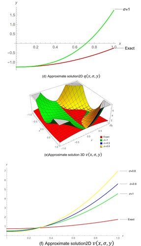
Figure 3. Comparison between Exact solution and approximate solution Example 3. (a) Approximate solution 3D $w\left(x,\sigma ,y\right)$. (b) Approximate solution2D $w\left(x,\sigma ,y\right)$. (c) Approximate solution 3D $q\left(x,\sigma ,y\right)$. (d) Approximate solution2D $q\left(x,\sigma ,y\right)$. (e)Approximate solution 3D $v\left(x,\sigma ,y\right)$. (f) Approximate solution2D $v\left(x,\sigma ,y\right).$

Table

Full names	Abbreviation
Elzaki Adomian decomposition method.	(EADM)
Fractional-order partial differential equations.	(FODEs)
Fractional partial differential equations.	(FDEs)
Homotopy perturbation methodology.	(HPM)
Laplace Adomian decomposition method.	(LADM)
Adomian decomposition method.	(ADM)

Availability of data and material

On request for supporting data, the authors will provide the study’s findings.

Authors’ contributions

We all looked at the document and came to an agreement on the final version.

Acknowledgements

We’d like to thank the Department of Mathematics for their assistance.

Disclosure statement

No potential conflict of interest was reported by the author(s).

References

- Subramanian M, Manigandan M, Tunç C, et al. On system of nonlinear coupled differential equations and inclusions involving Caputo-type sequential derivatives of fractional order. Journal of Taibah University for Science. 2022;16(1):1–23.
- Talib I, Raza A, Atangana A, et al. Numerical study of multi- order fractional differential equations with constant and variable coefficients. Journal of Taibah University for Science. 2022;16(1):608–620.
- Jothimani K, Kaliraj K, Hammouch Z, et al. New results on controllability in the framework of fractional integro differential equations with nondense domain. Eur Phys J Plus. 2019;134(9):441.
- Khan H, Shah R, Kumam P, et al. Analytical solutions of fractional-order heat and wave equations by the natural transform decomposition method. Entropy. 2019;21:597.
- Cherif MH, Ziane D, Belghaba K. Fractional natural decomposition method for solving fractional system of nonlinear equations of unsteady flow of a polytropic gas. Nonlinear Stud. 2018;25:753–764.
- Mohamed MZ, Hamza AE, Sedeeg AKH. An efficient approximate solutions of the fractional coupled Burger’s equation by conformable double Sumudu transforms. Ain Shams Journal. 2022;16:101–879.
- Mohamed MZ, Elzaki TM. Applications of new integral transform for linear and nonlinear fractional partial differential equations. Journal of King Saud University Science. 2020;32(1):544–549.
- Ahmed SA, Elzaki TM, Elbadri M, et al. Solution of partial differential equations by new double integral transform (Laplace – Sumudu transform). Ain Shams Eng J. 2021;12(4):4045–4049.
- Jagdev S, Devendra K, Dutt PS, et al. An efficient numerical approach for fractional multi-dimensional diffusion equations with exponential memory. Numer Methods Partial Diff Eqs. 2021;37(2):1631–1651.
- Mollahasani N, Moghadam MMM, Afrooz K. A new treatment based on hybrid functions to the solution of telegraph equations of fractional order. Appl Math Model. 2016;40:2804–2814.
- Khan H, Shah R, Kumam P, et al. Analytical solutions of fractional-order heat and wave equations by the natural transform decomposition method. Entropy. 2019;21(6):597.
- Shah R, Khan H, Mustafa S, et al. Analytical solutions of fractional-order diffusion equations by natural transform decomposition method. Entropy. 2019;21(6):557.
- Mohammed OH, Wadi Q. A modified method for solving delay differential equations of fractional order. IOSR J Math. 2016;12(3):15–21.
- Darzi R, Agheli B. Analytical approach to solving fractional partial differential equation by optimal q-homotopy analysis method. Numer Anal Appl. 2018;11(2):134–145.
- Al-Sabbagh AA, Hanan IK, Mohammed OH. Some numerical methods for solving fractional parabolic partial differential equations. Eng Technol J. 2010;28(12):2480–2485.
- Khan Y, Vazquez-Leal H, Faraz N. An auxiliary parameter method using Adomian polynomials and Laplace transformation for nonlinear differential equations. Appl Math Model. 2013;37(5):2702–2708.
- Nofal TA. Simple equation method for nonlinear partial differential equations and its applications. J Egypt Math Soc. 2016;24(2):204–209.
- Jafari H, Nazari M, Baleanu D, et al. A new approach for solving a system of fractional partial differential equations. Comput Math Appl. 2013;66(5):838–843.
- Sirisubtawee S, Koonprasert S. Exact traveling wave solutions of certain nonlinear partial differential equations using the-expansion method. Adv Math Phys. 2018.
- Chu Y-M, Khan MF, Ullah S, et al. Mathematical assessment of a fractional-order vector–host disease model with the Caputo–Fabrizio derivative. Math Meth Appl Sci. 2022.
- Rubbab Q, Nazeer M, Ahmad F, et al. Numerical simulation of advection–diffusion equation with caputo-fabrizio time fractional derivative in cylindrical domains: applications of pseudo-spectral collocation method. Alexandria Eng J. 2021;60(1):1731–1738.
- Jin F, Qian Z-S, Chu Y-M, et al. On nonlinear evolution model for drinking behavior under caputo-fabrizio derivative. J Appl Anal Comput. 2022;12(2):790–806.
- Vanani SK, Aminataei A. Tau approximate solution of fractional partial differential equations. Comput Math Appl. 2011;62(3):1075–1083.
- Ozpınar F. Applying discrete homotopy analysis method for solving fractional partial differential equations. Entropy. 2018;20(5):332.
- Shah R, Khan H, Kumam P, et al. An analytical technique to solve the system of nonlinear fractional partial differential equations. Mathematics. 2019;7(6):505.
- Khan H, Shah R, Kumam P, et al. An efficient analytical technique, for the solution of fractional-order telegraph equations. Mathematics. 2019;7(5):426.
- Almusawa H, Jhangeer A. Nonlinear self-adjointness, conserved quantities and Lie symmetry of dust size distribution on a shock wave in quantum dusty plasma. Commun Nonlinear Sci Numer Simul. 2022;114:1007–5704.
- Samina S, Jhangeer A, Chen Z. A study of phase portraits, multistability and velocity profile of magneto-hydrodynamic Jeffery–Hamel flow nanofluid. Chin J Phys. 2022: 0577–9073.
- Riaz MB, Jhangeer A, Atangana A, et al. Supernonlinear wave, associated analytical solitons, and sensitivity analysis in a two-component Maxwellian plasma. Journal of King Saud University – Science. 2022;34(5):1018–3647.
- Jhangeer A, Hussain A, Junaid-U-Rehman M, et al. Quasi-periodic, chaotic and travelling wave structures of modified Gardner equation. Chaos, Solitons Fractals. 2021;143:110578.
- Jafari HK, Nazari CM. Application of the Laplace decomposition method for solving linear and nonlinear fractional diffusion-wave equations. Appl Math Lett. 2011;24(11):1799–1805.
- Mohamed MZ, Elzaki TM. Comparison between the Laplace decomposition method and Adomian decomposition in time-space fractional nonlinear fractional differential equations. Appl Math. 2018;09(04):448.
- Gaxiola OG. The Laplace–Adomian decomposition method applied to the Kundu–Eckhaus equation. Int J Math Appl. 2017;5(1):1–12.
- Al-Zurigat M. Solving nonlinear fractional differential equation using a multi-step Laplace Adomian decomposition method. An Univ Craiova Ser Mat Inform. 2012;39(2):200–210.
- Ohammed OH, Salim HA. Computational methods based Laplace decomposition for solving nonlinear system of fractional order differential equations. Alex Eng J. 2018;57(4):3549–3557.
- Shah HF, ur Rahman K, Shahzad M G. Numerical solution of fractional order smoking model via Laplace Adomian decomposition method. Alex Eng J. 2018;57(2):1061–1069.
- Mahmood S, Shah R, Arif M. Laplace Adomian decomposition method for multi dimensional time fractional model of Navier–Stokes equation. Symmetry (Basel). 2019;11(2):149.
- Shah R, Khan H, Arif M, et al. Application of Laplace–Adomian decomposition method for the analytical solution of third-order dispersive fractional partial differential equations. Entropy . 2019;21(4):335.
- Miller KS, Ross B. An introduction to the fractional calculus and fractional differential equations; 1993.
- Tayyaba A, Muhammad A, Bilal RM, et al. An efficient numerical technique for solving time fractional Burgers equation. Alexandria Eng J. 2020;59:2201–2220.
- Sene N. Second-grade fluid with Newtonian heating under Caputo fractional derivative: analytical investigations via Laplace transforms. Mathematical Modelling and Numerical Simulation with Applications. 2022;2(1):13–25.
- Khan H, Shah R, Kumam P, et al. Laplace decomposition for solving nonlinear system of fractional order partial different equations. Adv Differ Equ. 2020: 2020–2375.