The q-homotopy analysis method for a solution of the Cahn–Hilliard equation in the presence of advection and reaction terms

Abstract

In this paper, we provide a solution to the Cahn–Hilliard equation using the q-homotopy analysis method (q-HAM). The q-HAM is a more general, simple and widely used method for solving stiff nonlinear partial differential equations. The Cahn–Hilliard equation is a classical model in material sciences that describe spinodal decomposition and phase separation in two-phase flows. Using the q-HAM, the effect of various parameters of physical interest such as diffusive parameter, thickness parameter, advection and reaction terms on concentration is studied. The comparison of the computed solution with the exact solution is presented for some fixed parameter values to validate the solution obtained using the q-HAM.

KEYWORDS:

• The Cahn–Hilliard equation
• the q-homotopy analysis method
• advection and reaction terms
• thickness of transition layer
• diffusion parameter

1. Introduction

Many natural and physical phenomena can be described by reaction, diffusion and advection to describe a variety of physical and chemical processes arising in various fields of sciences and engineering, such as the flow of heat, wave propagation on shallow water, movement of electricity in conductors, the flow of fluids, plasma physics, chemical reactions and quantum mechanical systems. The mathematical modelling of such problems leads to nonlinear partial differential equations (PDEs). These models play a vital role in studying the physical behaviour of such types of natural phenomena. Numerous mathematical models and their solutions have been discussed in the literature, such as Wazwaz–Benjamin–Bona–Mahony equation, Schrödinger equation, diffusion equation, geophysical Korteweg–de Vries equation, Regularized Long Wave equations, Ablowitz-Kaup-Newell-Segur water wave dynamical equation, etc. [1–12]. These models introduce new ideas about the relations of diffusion, reaction, advection and nonlinearity.

The Cahn–Hilliard (CH) equation was introduced by American mathematicians and scientists Cahn and Hilliard [13]. It is an important mathematical model of mathematical physics that describes phase separation processes like spinodal decomposition in multi-phase systems. The nonlinear nature of the CH equation makes it difficult to find its exact solution. It becomes more complicated when it contains diffusion parameters, advection parameters, interface thickness parameters and reaction terms. An essential and important characteristic of the CH equation is the interface thickness between two phases that has a finite thickness. In the literature, researchers and scientists explore and analyse various forms of the CH equation with its applications in different fields of engineering and sciences [14–22]. Bouhassoun and Cherif [23] analyse the fractional form of the CH equation using the homotopy perturbation method. Tripathi et al. [24] discuss the solution of the time-fractional CH equation with reaction term using the homotopy analysis method. Zhu et al. [25] reported the solution of the CH equation with variable mobility. Barrett et al. [26] studied the solution behaviour of the CH equation with degenerate mobility. Berti and Bochiccchio [27] discussed generalized CH equation including thermal and mixing effects. Colby et al. [28] used the adaptive neural networks approach for solving the Allen Cahn and the CH equations numerically. A. Shah and A. A Siddiqui [29] used the variational iteration method to solve the viscous CH equation. S. Hussain and A. Shah [30] applied the homotopy perturbation method and variational iteration method to solve the CH equation. It is known that the exact analytical solution of the CH equation is difficult to obtain due to the sharp interface width and jump discontinuity at the interface. The literature review reveals that the CH equation with parameters of physical interest is not studied extensively due to its complicated nature. Therefore, we propose a series solution to the CH equation using the q-HAM. We also explore the effect of different parameters on concentration. To validate the computed results, we compare the solution with the existing one [31] for some fixed value of the parameters. The graphical illustrations of the results are also given.

2. Mathematical model

The generalized form of the CH equation [25–27] is (1) $\frac{\mathrm{\partial }u}{\mathrm{\partial }t}=\mathrm{\Gamma }\frac{{\mathrm{\partial }}^2}{\mathrm{\partial }{x}^2}\left(u^3-u-\gamma \frac{{\mathrm{\partial }}^{2}u}{\mathrm{\partial }{x}^2}\right)+\beta \frac{\mathrm{\partial }u}{\mathrm{\partial }x}+ku(1-u)\text{.}$(1) In Equation (1), $\mathrm{\Gamma }$ is the diffusion parameter, $\gamma$ is the thickness of the transition region, $\beta$ is the coefficient of the advection term and $k$ is the coefficient of the reaction term.

3. The q-HAM

In 2012, Tawil and Huseen [32] introduced the modified version of the Homotopy Analysis Method known as q-HAM for solving several nonlinear PDEs. They proved that HAM is a special case of q-HAM [33]. However, q-HAM is fast convergent with a large convergence region including other advantages over HAM. It also provides a more appropriate approach to tackle the region of convergence.

3.1. Basic idea of q-HAM

To understand the key idea of q-HAM, consider the nonlinear equation of the following form (2) $\mathrm{N}[\mathrm{\Psi }(x,t)]-v(x,t)=0\text{,}$(2) where $\mathrm{N}$ is a nonlinear operator, “$v$” is a known function and “$\mathrm{\Psi }$” is an unknown function with x and t as independent variables. Let us make the zeroth-order deformation equation as follows (3) $\begin{array}{rl}& (1-mq)L[\mathrm{\Psi }(x,t;q)-{\mathrm{\Psi }}_0(x,t)]\\ & =q\hslash \mathrm{H}(x,t)(\mathrm{N}[\mathrm{\Psi }(x,t;q)]-v(x,t))=0.\end{array}$(3) where $\hslash$ is a non-zero auxiliary parameter, $q\in [0,\frac{1}{m}]$ is the embedding parameter, $\mathrm{H}(x,t)$ is the auxiliary function, ${\mathrm{\Psi }}_0(x,t)$ is the initial solution of $\mathrm{\Psi }(x,t)$ and $L$ is a linear operator. When $v(x,t)=0$ and $q=0$ and $q=\frac{1}{m}$, Equation (3) gives, $\mathrm{\Psi }(x,t;0)={\mathrm{\Psi }}_0(x,t)$ and $\mathrm{\Psi }\left(x,t;\frac{1}{m}\right)=\mathrm{\Psi }(x,t)$, respectively.

Now expanding $\mathrm{\Psi }(x,t;q)$ with respect to $q$ using the Taylor series, we have (4) $\mathrm{\Psi }(x,t;q)={\mathrm{\Psi }}_0(x,t)+\sum _{n=1}^{\mathrm{\infty }}{\mathrm{\Psi }}_n(x,t)q^n\text{,}$(4) where (5) ${\mathrm{\Psi }}_n(x,t)={\frac{1}{n!}\frac{{\mathrm{\partial }}^n\mathrm{\Psi }(x,t)}{\mathrm{\partial }{q}^n}|}_{q=0}\text{.}$(5) If one chooses the linear operator $L$, auxiliary parameter $\hslash$, auxiliary function $\mathrm{H}(x,t)$ and initial approximation ${\mathrm{\Psi }}_0(x,t)$ properly, the series in Equation (4) converges, then we get (6) $\mathrm{\Psi }(x,t)={\mathrm{\Psi }}_0(x,t)+\sum _{n=1}^{\mathrm{\infty }}{\mathrm{\Psi }}_n(x,t){\left(\frac{1}{m}\right)}^n\text{.}$(6) Define the vector (7) $\overrightarrow{\mathrm{\Psi }}(x,t)=\{{\mathrm{\Psi }}_0(x,t),{\mathrm{\Psi }}_1(x,t),{\mathrm{\Psi }}_2(x,t),\dots ,{\mathrm{\Psi }}_n(x,t)\}\text{,}$(7) then $n^{th}$ order deformation equation obtained using Equation (3) is given by (8) $L[{\mathrm{\Psi }}_n(x,t)-{\lambda }_n{\mathrm{\Psi }}_{n-1}]=\hslash \mathrm{H}(x,t)\{R_n[{\overrightarrow{\mathrm{\Psi }}}_{n-1}(x,t)]\}\text{.}$(8) where (9) $R_n[{\overrightarrow{\mathrm{\Psi }}}_{n-1}(x,t)]=\frac{1}{(n-1)!}\frac{{\mathrm{\partial }}^{n-1}\mathrm{N}[\mathrm{\Psi }(x,t;q)]}{\mathrm{\partial }{q}^{n-1}}\text{,}$(9) and (10) ${\lambda }_n=\{\begin{array}{l}0\text{when}n=1,\\ 1\text{when}n>1.\end{array}$(10) Applying $L^{-1}$ on both sides of Equation (8) and after simplification, we get (11) ${\mathrm{\Psi }}_n(x,t)=\hslash L^{-1}[\mathrm{H}(x,t)\{R_n[{\overrightarrow{\mathrm{\Psi }}}_{n-1}(x,t)]\}]+{\lambda }_n{\mathrm{\Psi }}_{n-1}\text{.}$(11) Using Equation (11) one can approximate the analytical solution $\mathrm{\Psi }(x,t)$ of the following form (12) $\mathrm{\Psi }(x,t)=\sum _{n=0}^N{\mathrm{\Psi }}_n(x,t){\left(\frac{1}{m}\right)}^n\text{.}$(12) Due to the presence of a factor ${\left(\frac{1}{m}\right)}^n$, q-HAM converges faster than HAM.

4. Numerical experiments

In this section, we solve the CH equation with the given initial conditions.

4.1. Example

Consider the CH equation of the following form [24] (13) $u_t-\mathrm{\Gamma }(u^3-u-\gamma u_{xx}{)}_{xx}-\beta u_x-k(u-u^2)=0,$(13) with the initial condition (14) $u(x,0)=x\text{.}$(14) By considering the initial condition as an initial guess, we have (15) $u_0(x,t)=x\text{.}$(15) Using Equations (13) and (14) in Equations (9) and (11), we get the first approximation as (16) $u_1(x,t)=-h\text{t(}-k{x}^2\text{ + 6}\mathrm{\Gamma }x\text{ + }kx\text{ + }\beta \text{)}\text{.}$(16)

Similarly, the second and third iterations are (17) $\begin{array}{rl}& u_2(x,t)=54ht\\ & \left[\begin{array}{l}\left(\begin{array}{l}\frac{k^{\text{2}}t{x}^3}{\text{54}}+\left(-\frac{\text{4}\mathrm{\Gamma }k\text{t}}{\text{9}}-\frac{k^{\text{2}}t}{\text{36}}\text{ + }\frac{k}{\text{54}}\right)x^2\\ +\left(\frac{k^{2}t}{108}+\left(-\frac{1}{54}+\left(\frac{2\mathrm{\Gamma }}{9}-\frac{\beta }{27}\right)t\right)k+{\mathrm{\Gamma }}^{2}t-\frac{\mathrm{\Gamma }}{9}\right)x\\ +\frac{t(\mathrm{\Gamma }+\beta )k}{54}+\frac{\mathrm{\Gamma }t\beta }{9}-\frac{\beta }{54}\end{array}\right)h\\ -\frac{n}{9}\left(-\frac{k{x}^2}{6}+\left(\mathrm{\Gamma }+\frac{k}{6}\right)x+\frac{\beta }{6}\right)\end{array}\right]\text{,}\end{array}$(17) (18) $\begin{array}{rl}& u_3(x,t)=-540ht\\ & [\left(\begin{array}{c}\left(\begin{array}{c}-\frac{1}{540}(x-1)\left(x^2-x+\frac{1}{6}\right)x{k}^3\\ +\left(\begin{array}{c}\frac{\mathrm{\Gamma }{x}^3}{9}+\left(-\frac{31\mathrm{\Gamma }}{270}+\frac{\beta }{180}\right)x^2+\left(\frac{31\mathrm{\Gamma }}{1620}-\frac{\beta }{180}\right)x\\ +\frac{\mathrm{\Gamma }}{405}+\frac{\beta }{1080}\end{array}\right)k^2\\ +\left(-\frac{8{\mathrm{\Gamma }}^2{x}^2}{9}+\frac{3\mathrm{\Gamma }}{10}\left(-\frac{8\beta }{27}+\mathrm{\Gamma }\right)x+\frac{{\mathrm{\Gamma }}^2}{30}-\frac{{\beta }^2}{540}+\frac{\mathrm{\Gamma }\beta }{45}\right)k\\ +{\mathrm{\Gamma }}^2\left(\mathrm{\Gamma }x+\frac{\beta }{10}\right)\end{array}\right)t^2\\ +\left(\begin{array}{c}-\frac{1}{270}(x-1)\left(x-\frac{1}{2}\right)x{k}^2+\left(\begin{array}{c}\frac{4\mathrm{\Gamma }{x}^2}{45}+\left(-\frac{2\mathrm{\Gamma }}{45}+\frac{\beta }{135}\right)x\\ -\frac{\beta }{270}-\frac{\mathrm{\Gamma }}{270}\end{array}\right)k\\ -\frac{\mathrm{\Gamma }}{5}\left(\mathrm{\Gamma }x+\frac{\beta }{9}\right)\end{array}\right)\\ t-\frac{kx}{540}(x-1)+\frac{\beta }{540}+\frac{\mathrm{\Gamma }x}{90}\end{array}\right)\\ & h^2+\dots +\frac{n^2}{90}\left(\begin{array}{c}\left(-\frac{x^2}{6}+\frac{x}{6}\right)k\\ +\frac{\beta }{6}+Dx\end{array}\right)\phantom{\left(\begin{array}{c}\left(\begin{array}{c}-\frac{1}{540}(x-1)\left(x^2-x+\frac{1}{6}\right)x{k}^3\\ +\left(\begin{array}{c}\frac{\mathrm{\Gamma }{x}^3}{9}+\left(-\frac{31\mathrm{\Gamma }}{270}+\frac{\beta }{180}\right)x^2+\left(\frac{31\mathrm{\Gamma }}{1620}-\frac{\beta }{180}\right)x\\ +\frac{\mathrm{\Gamma }}{405}+\frac{\beta }{1080}\end{array}\right)k^2\\ +\left(-\frac{8{\mathrm{\Gamma }}^2{x}^2}{9}+\frac{3\mathrm{\Gamma }}{10}\left(-\frac{8\beta }{27}+\mathrm{\Gamma }\right)x+\frac{{\mathrm{\Gamma }}^2}{30}-\frac{{\beta }^2}{540}+\frac{\mathrm{\Gamma }\beta }{45}\right)k\\ +{\mathrm{\Gamma }}^2\left(\mathrm{\Gamma }x+\frac{\beta }{10}\right)\end{array}\right)t^2\\ +\left(\begin{array}{c}-\frac{1}{270}(x-1)\left(x-\frac{1}{2}\right)x{k}^2+\left(\begin{array}{c}\frac{4\mathrm{\Gamma }{x}^2}{45}+\left(-\frac{2\mathrm{\Gamma }}{45}+\frac{\beta }{135}\right)x\\ -\frac{\beta }{270}-\frac{\mathrm{\Gamma }}{270}\end{array}\right)k\\ -\frac{\mathrm{\Gamma }}{5}\left(\mathrm{\Gamma }x+\frac{\beta }{9}\right)\end{array}\right)\\ t-\frac{kx}{540}(x-1)+\frac{\beta }{540}+\frac{\mathrm{\Gamma }x}{90}\end{array}\right)}]\text{.}\end{array}$(18) Continuing in the same line, we can find $u_4,u_5,\dots$ up to the required number of iterations.

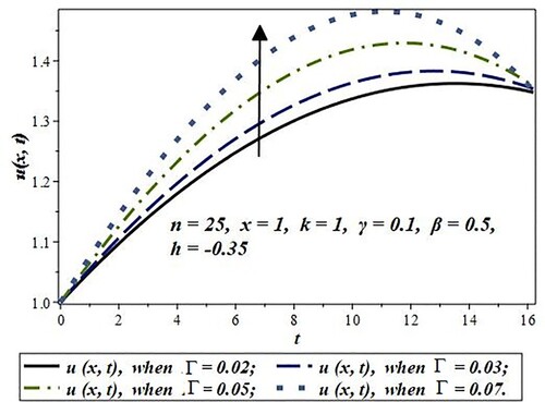
4.1.1. Effect of diffusion on concentration

In Figure 1, the effect of diffusion parameter “$\mathrm{\Gamma }$” on concentration has been studied for different values. It is clear from the figure that the concentration increases with the increase of diffusion.

Figure 1. Effect of the diffusion parameter “$\mathrm{\Gamma }$” on concentration $u(x,t)$ for $\mathrm{\Gamma }$=  0.02, 0.03, 0.05 and 0.07.

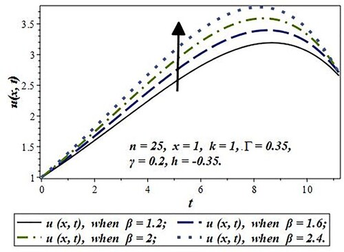
4.1.2. Effect of thickness on concentration

In Figure 2, the effect of the thickness parameter “$\gamma$” on concentration is depicted by taking various values of the thickness parameter. From Figure 2, one can conclude that the thickness parameter is directly proportional to the concentration.

Figure 2. Effect of the thickness parameter “$\gamma$” on concentration $u(x,t)$ for $\gamma =0.01,0.5,1.5,2.5$.

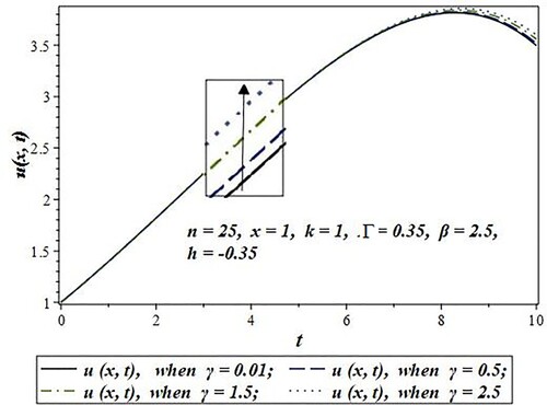
4.1.3. Effect of advection on concentration

In Figure 3, the effect of the advection parameter “$\beta$” on concentration is represented by taking various values of the advection parameter. From Figure 3 we can observe that the concentration upsurges with the increase of advection.

Figure 3. Effect of the advection parameter “$\beta$” on concentration $u(x,t)$ for $\beta =1.2,1.6,2,2.4$.

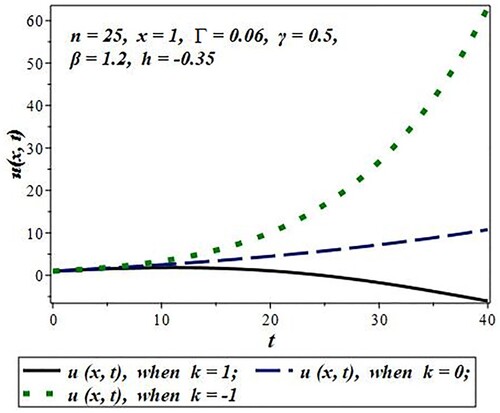
4.1.4. Effect of reaction term on concentration

In Figure 4, the effect of the reaction parameter “$k$” on concentration is validated by taking various values of “k”. It is observed that the concentration enhances in the presence of the source term i.e. $k=1$. Whereas, the concentration decreases in the presence of sink term i.e. $k=-1$, while a very small increase in concentration is observed in the absence of source and sink term i.e. $k=0$.

Figure 4. Effect of the reaction parameter “$k$” on concentration $u(x,t)$ for $k=1,0,-1$.

4.1.5. Convergence analysis

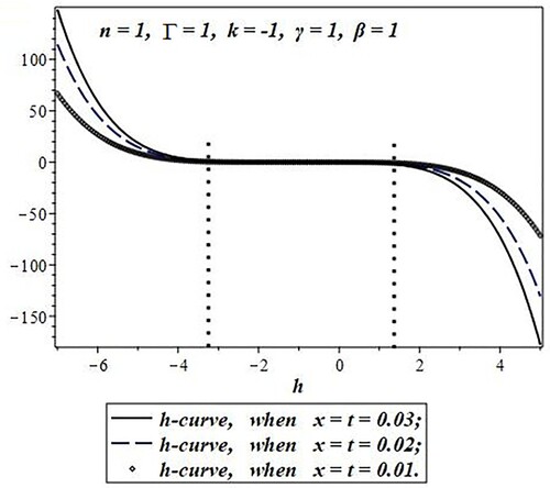
In order to calculate the effective region of “h”, the h-curves are plotted for different values of independent variables “x” and “t”. From Figures 6–8, it can be observed that q-HAM provides a large convergence region as compared to the classical HAM, as shown in Figure 5.

Figure 5. h-curve for the HAM (q-HAM, when n = 1) approximate solution after the sum of the first five iterations $u_0+u_1+\cdots +u_5$.

From Figures 5–8, it can be observed that the convergence region of parameter “h” increases with the increase of “n”. Table 1 states the convergence region of parameter “h” with the increase of “n”.

Figure 6. h-curve for the q-HAM (when n = 5) approximate solution after the sum of the first five iterations $u_0+u_1+\cdots +u_5$.

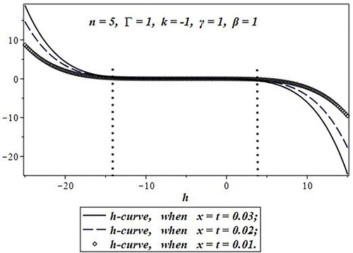
Figure 7. h-curve for the q-HAM (when n = 10) approximate solution after the sum of the first five iterations $u_0+u_1+\cdots +u_5$.

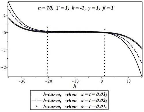
Figure 8. h-curve for the q-HAM (when n = 20) approximate solution after the sum of the first five iterations $u_0+u_1+\cdots +u_5$.

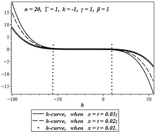
Table 1. Convergence region of “h” for different values of “n”.

n	h
1(HAM)	$-3.257\le h\le 1.317$
5	$-14.076\le h\le 3.908$
10	$-20.242\le h\le 1.344$
20	$-55.302\le h\le 9.943$

4.2. Numerical comparison

In this section, we compare computed results with the results obtained in [31] through absolute error analysis taking $\mathrm{\Gamma }=1,\beta =1,\gamma =1\text{and}k=0$ in Equation (13). (19) $u_t-(u^3-u-u_{xx}{)}_{xx}-u_x=0.$(19) The exact solution of Equation (19) is given as [31] (20) $u(x,t)=\tanh \left(\frac{x+t}{\sqrt{2}}\right)\text{.}$(20) To implement q-HAM, consider $u(x,0)=u_0(x,t)$ as an initial guess (21) $u_0(x,t)=\tanh \left(\frac{x}{\sqrt{2}}\right)\text{.}$(21) Using Equations (20) and (21) in Equations (9) and (11), we get the first approximation as (22) $u_1(x,t)=-\frac{ht\sqrt{2}}{2{\cosh }^2\left(\frac{x\sqrt{2}}{2}\right)}\text{.}$(22) Similarly, the second and third iterations are (23) $\begin{array}{rl}{u}_2(x,t)& =-\frac{ht}{2{\cosh }^3\left(\frac{x\sqrt{2}}{2}\right)}[\sqrt{2}(h+n)\cosh \left(\frac{x\sqrt{2}}{2}\right)\\ & +ht\sinh \left(\frac{x\sqrt{2}}{2}\right)]\text{,}\end{array}$(23) (24) $\begin{array}{rl}& u_3(x,t)=-\frac{ht}{6{\cosh }^4\left(\frac{x\sqrt{2}}{2}\right)}\\ & \left[\begin{array}{c}\sqrt{2}((t^2+3)h^2+6hn+3n^2){\cosh }^2\left(\frac{x\sqrt{2}}{2}\right)\\ +6ht\sinh \left(\frac{x\sqrt{2}}{2}\right)(h+n)\cosh \left(\frac{x\sqrt{2}}{2}\right)-\frac{3\sqrt{2}{h}^2{t}^2}{2}\end{array}\right]\text{.}\end{array}$(24) Proceeding in the same manner we can calculate $u_4,u_5,\dots$.

4.2.1. Convergence analysis

The valid region for convergence parameter “h” is studied for different values of “n”. It is observed that the convergence region increases with the increase in “n”. The results are elaborated in Table 2.

Table 2. Convergence region of h-curve for $x=t=0.1,0.2,0.3$.

n	h
1 (HAM)	$-3.987\le h\le 2.439$
5	$-13.383\le h\le 5.215$
10	$-40.878\le h\le 14.646$
20	$-84.505\le h\le 43.245$
30	$-164.179\le h\le 108.313$
40	$-166.097\le h\le 120.213$
50	$-236.359\le h\le 154.553$

4.2.2. Error analysis

In Table 3, the absolute error is calculated for different values of “x” and “t”. The table illustrates the convergence of the approximate solution obtained using the q-HAM.

Table 3. Absolute between exact solution [31] and approximate solution by q-HAM for $n=10$ and $h=-10.223$.

	t
x	0.01	0.02	0.03	0.04	0.05
0.1	$1\times {10}^{-11}$	$6\times {10}^{-11}$	$6\times {10}^{-11}$	$6.1\times {10}^{-10}$	$7.8\times {10}^{-9}$
0.2	$6\times {10}^{-10}$	$2\times {10}^{-10}$	$7\times {10}^{-10}$	$7\times {10}^{-10}$	$2.6\times {10}^{-9}$
0.3	$2\times {10}^{-10}$	$5\times {10}^{-10}$	$4\times {10}^{-10}$	$2.7\times {10}^{-9}$	$1.49\times {10}^{-8}$
0.4	$3\times {10}^{-10}$	$8\times {10}^{-10}$	$1.6\times {10}^{-9}$	$8.6\times {10}^{-9}$	$2.1\times {10}^{-9}$
0.5	$1\times {10}^{-10}$	$9\times {10}^{-10}$	$2.4\times {10}^{-9}$	$1.05\times {10}^{-8}$	$2\times {10}^{-9}$

5. Conclusion

In this work, the effect of various parameters of practical interest on the concentration of the multi-phase system described by the CH equation is investigated. The effect of each parameter is illustrated in Figures 1–4. The q-HAM is used to obtain the series solution of the CH equation. The convergence of the h-curve is also studied through Figures 5–8 and Table 1 for increasing values of “n”. Table 2 gives the range of solution controlling parameter “h” for higher “n”. It is clear from Tables 1 and 2 that the q-HAM provides a large range of “h” as compared to HAM. It also suggests that HAM is a special case of q-HAM when n = 1. The comparison of exact and approximate solutions is also provided using the absolute error. Table 3 validates the application of q-HAM for solving the CH equation involving various parameters of physical importance. The following key observations are made in the light of obtained solutions.

• It is observed that concentration increases with the increase of diffusion.

• Concentration increases the increase of thickness parameter.

• Concentration is directly proportional to the advection parameter.

• The results of the reaction term reveal that concentration upsurges in the presence of source term i.e. $k=1$. Concentration decreases in the presence of sink term i.e. $k=-1$. While a very small increase in concentration is observed in the absence of source and sink term i.e. $k=0$.

In future work, we will use some numerical techniques such as finite difference schemes and finite element techniques to simulate and study the effect of above-stated parameters.

Disclosure statement

No potential conflict of interest was reported by the author(s).

References

- Akram U, Aly RS, Rizvi STR, et al. Traveling wave solutions for the fractional Wazwaz–Benjamin–Bona–Mahony model in arising shallow water waves. Results Phys. 2021;20:103725. doi:10.1016/j.rinp.2020.103725.
- Rizvi ST, Seadawy AR, Ashraf F, et al. Lump and interaction solutions of a geophysical Korteweg–de Vries equation. Results Phys. 2020;19:Article 103661. doi:10.1016/j.rinp.2020.103661.
- Younas U, Younis M, Aly RS, et al. Diverse exact solutions for modified nonlinear Schrödinger equation with conformable fractional derivative. Results Phys. 2021;20(8):Article 103766. doi:10.1016/j.rinp.2020.103766.
- Younis M, Ali S, Rizvi STR, et al. Investigation of solitons and mixed lump wave solutions with (3 + 1)-dimensional potential-YTSF equation. Commun Nonlinear Sci Numer Simul. 2021;94:Article 105544. doi:10.1016/j.cnsns.2020.105544.
- Ali A, Seadawy AR, Lu D. Soliton solutions of the nonlinear Schrödinger equation with the dual power law nonlinearity and resonant nonlinear schrödinger equation and their modulation instability analysis. Optik (Stuttg). 2017;145:79–88. doi:10.1016/j.ijleo.2017.07.016.
- Aly RS, Younis M, Baber MZ, et al. Diverse acoustic wave propagation to confirmable time–space fractional KP equation arising in dusty plasma. Commun Theor Phys. 2021;73(11):Article 115004.
- Younis M, Nadia C, Mahmood AS, et al. A variety of exact solutions to (2 + 1)-dimensional schrödinger equation. Waves Random Complex Media. 2018;30:1–10. doi:10.1080/17455030.2018.1532131.
- Asghar A, Seadawy AR, Dianchen L. Computational methods and traveling wave solutions for the fourth-order nonlinear Ablowitz-Kaup-Newell-Segur water wave dynamical equation via two methods and its applications. Open Physics. 2018;16(1):219–226. DOI: 10.1515/phys-2018-0032.
- Dianchen L, Seadawy AR, Asghar A. Applications of exact traveling wave solutions of modified Liouville and the symmetric regularized long wave equations via two new techniques. Results Phys. 2018;9:1403–1410. doi:10.1016/j.rinp.2018.04.039.
- Asghar A, Seadawy AR, Dianchen L. Dispersive solitary wave soliton solutions of (2 + 1)-dimensional Boussinesq dynamical equation via extended simple equation method. J King Saud Univ Sci. 2019;31(4):653–658. doi:10.1016/j.jksus.2017.12.015.
- Alruwaili AD, Seadawy AR, Asghar A, et al. Novel analytical approach for the space-time fractional (2 + 1)-dimensional breaking soliton equation via mathematical methods. Mathematics. 2021;9:3253. doi:10.3390/math9243253.
- Alruwaili AD, Seadawy AR, Ali A, et al. Soliton solutions of Calogero– Degasperis–Fokas dynamical equation via modified mathematical methods. Open Physics. 2022;20:174–187. DOI: 10.1515/phys-2022-0016.
- Cahn JW, Hilliard J. Free energy of a nonuniform system. I. interfacial free energy. J Chem Phys. 1958;28:258–267.
- Bertozzi AL, Esedoglu S, Gillette A. Inpainting of binary images using the Cahn-Hilliard equation. IEEE Trans Image Process. 2007;16(1):285–291. doi:10.1109/TIP.2006.887728.
- Junseok K, Seunggyu L, Yongho C, et al. Basic principles and practical applications of the Cahn–Hilliard equation. Math Probl Eng. 2016: 11. Article ID 9532608. doi:10.1155/2016/9532608.
- Miranville A, Piétrus A, Rakotoson J. Dynamical aspect of a generalized Cahn–Hilliard equation based on a microforce balance. Asymptotic Anal. 1998;16:315–345. Corpus ID:118719560.
- Nicolaenko B, Scheurer B, Temam R. Some global dynamical properties of a class of pattern formation equations. Commun Partial Differ Equ. 1989;14(2):245–297. doi:10.1080/03605308908820597.
- Novick-Cohen A, Segel LA. Nonlinear aspects of the Cahn-Hilliard equation. Physica D. 1984;10:277–298. doi:10.1016/0167-2789(84)90180-5.
- Gurtin M. Generalised Ginzburg-Landau and Cahn-Hilliard equations based on a microforce balance. Physica D. 1996;92:178–192. doi:10.1016/0167-2789(95)00173-5.
- Choksi R, Peletier MA, Williams JF. On the phase diagram for microphase separation of diblock copolymers: an approach via a nonlocal Cahn–Hilliard functional. SIAM J Appl Math. 2009;69:1712–1738. Doi:10.1137/080728809.
- Tang P, Qiu F, Zhang H, et al. Phase separation patterns for diblock copolymers on spherical surfaces: a finite volume method. Phys Rev E Stat Nonlin Soft Matter Phys. 2005;72:016710. doi:10.1103/PhysRevE.72.016710.
- Hu SY, Chen LQ. A phase-field model for evolving microstructures with strong elastic inhomogeneity. Acta Mater. 2001;49:1879–1890. doi:10.1016/S1359-6454(01)00118-5.
- Bouhassoun A, Cherif H. Homotopy perturbation method For solving The fractional Cahn-Hilliard equation. J Interdiscip Math. 2015;18:513–524. doi:10.1080/10288457.2013.867627.
- Tripathi NK, Das S, Ong SH, et al. Solution of time-fractional Cahn–Hilliard equation with reaction term using homotopy analysis method. Adv Mech Eng. 2017;9:168781401774077. doi:10.1177/1687814017740773.
- Zhu J, Long-Qing C, Shen J, et al. Coarsening kinetics from a variable-mobility Cahn-Hilliard equation: application of a semi-implicit Fourier spectral method. Phys Rev E Stat Phys Plasmas Fluids Relat Interdiscip Topics. 1999;60:3564–3572. doi:10.1103/PhysRevE.60.3564.
- Barrett J, Blowey J, Garcke H. Finite element approximation of the Cahn-Hilliard equation with degenerate mobility. SIAM J Numer Anal. 2000;37. doi:10.1137/S0036142997331669.
- Berti A, Bochicchio I. A mathematical model for phase separation: a generalized Cahn- Hilliard equation. Math Method Appl Sci. 2011;34:1193–1203. doi:10.1002/mma.1432.
- Wight CL, Zhao J. Solving Allen-Cahn and Cahn-Hilliard equations using the adaptive physics informed neural networks. Commun Comput Phys. 2021;29:930–954. doi:10.4208/cicp.OA-2020-0086.
- Shah A, Siddiqui AA. Variational iteration method for the solution of viscous Cahn-Hilliard equation. World Appl Sci J. 2010;11(7):813–818. Corpus ID: 16027042.
- Hussain S, Shah A. An analysis of two iterative techniques for solution of Cahn-Hilliard equation. Int J Nonlinear Sci. 2011;12(1):42–47.
- Ugurlu Y, Kaya D. Solutions of the Cahn–Hilliard equation. Comput Math Appl. 2008;56:3038–3045. doi:10.1016/j.camwa.2008.07.007.
- El-Tawil MA, Huseen S. The q-homotopy analysis method (q-HAM). Int J Appl Math Mech. 2012;8:51–75. Corpus ID:124341343.
- Liao SJ. Beyond perturbation: introduction to the homotopy analysis method. Boca Raton (FL): CRC Press, Chapman & Hall; 2003.