A novel scheme for the hyperbolic partial differential equation through Fibonacci wavelets

ABSTRACT

In this study, we generated the operational matrices of integration based on the Fibonacci wavelets through the concept of linear algebra and developed the novel technique known as the Fibonacci wavelet collocation method (FWCM). The proposed approach extracts the numerical solution of linear hyperbolic partial differential equations (HPDEs). This technique is an efficient and emerging numerical algorithm that converts the considered problem into a system of equations of algebraic type. We obtained desired numerical results in solving this system of algebraic equations with the help of the Newton–Raphson technique. We solved the five problems concerning a minimum level of resolution to strengthen our results. The obtained outcome is compared with the exact and other numerical solutions available in the literature through tables and graphs. The tables and graphical representations clarify the accuracy and efficiency of the proposed technique. Convergence analysis for the proposed method is drawn in terms of the theorems.

KEYWORDS:

• Hyperbolic partial differential equations
• Collocation method
• Operational matrix of integration
• Fibonacci wavelets
• Newton–Raphson technique

2010 MATHEMATICS SUBJECT CLASSIFICATIONS:

• 35L02
• 65M70
• 65T60

1. Introduction

A Partial differential equation (PDE) is the mathematical model of real-world physical, chemical, and biological problems and describes many physical phenomena in nature. In recent years, PDE has become a language of many fields such as thermodynamics, electrostatics, electrodynamics, elasticity, general relativity, quantum mechanics, sound, heat, traffic flow [1], electroshock therapy [2], medicine [3], waste-water treatment [4], chemical [5], fluid mechanics [6-8], engineering [9], and biology [10,11]. In the classification of PDEs, we considered three sorts of PDEs such as parabolic, hyperbolic, and elliptic. Out of these, the Hyperbolic type gets much more attention from researchers due to its tremendous applications in industry, atomic physics, biology, aerospace, and engineering problems such as vibrations of structures, beams, and buildings. The term “hyperbolic” was typically used to refer to a certain class of nth-order equations in the nomenclature of classical partial differential equations.

Consider an equation $a{U}_{xx}+b{U}_{xt}+c{U}_{tt}=0$, the coefficients $a,b,c$ depend on the values of $x$, the equation will be hyperbolic in a region if $b^2-4ac>0$. HPDEs are built as mathematical models that describe wave phenomena with more applications in various fields such as optical devices, earth sciences (oil exploration), electromagnetic radiation [12], fluid mechanics [13,14], and geosciences [15], applied mathematics, physics, and engineering. HPDEs come in various forms, such as the wave equation and the telegraph equation, etc. The wave equation describes waves like sound, water, and seismic waves that occur in classical physics. The solutions of these equations based on continuum mechanics are usually singular, including discontinuity, shock discontinuity, etc. For such models, anticipating the exact solution always is not possible. So, numerical techniques are employed to study those problems. To solve such equations, we need to pay a high computational cost and increased CPU burden, and it is complicated to solve engineering physics problems with a certain scale. In recent years researchers have been paying close attention to HPDEs’ solutions. To solve these hyperbolic equations, a variety of numerical techniques were offered, including semi-analytical methods, finite difference techniques, spectral methods, and finite element processes. Because of the above analysis and the special properties of HPDEs, people began to seek an efficient technique called the wavelet method to avoid these singular extreme points. Here wavelet techniques are very simple and minimises the computational cost. Due to this, we considered HPDE problems through the wavelet technique.

Consider the general form of the first-order linear hyperbolic equation (1) $\begin{array}{rl}& {\displaystyle \frac{\mathrm{\partial }S\left(x,t\right)}{\mathrm{\partial }t}}+{\displaystyle \frac{\mathrm{\partial }S\left(x,t\right)}{\mathrm{\partial }x}}+S\left(x,t\right)\\ & =f\left(x,t\right),0\le x\le 1,0\le t\le 1\end{array}$(1) subject to the conditions: (2) $\begin{array}{rl}& S\left(x,0\right)=p\left(x\right),S\left(0,t\right)=q\left(t\right),\\ & S\left(a,t\right)=r\left(t\right),0\le x\le 1,0\le t\le 1\end{array}$(2) This type of HPDE is solved through various methods [16-20]. We solve these hyperbolic equations by the Fibonacci wavelet collocation method.

Wavelet analysis is a new and emerging field in applied and computational numerical exploration. The subject of wavelet analysis has recently attracted a lot of interest from mathematicians across the world. Wavelets are mathematical functions that aid in dividing data into distinct recurrence sections and urge the exploration of each data segment with a goal proportional to its scale. Wavelets outperform traditional Fourier techniques when analyzing physical situations with discontinuities and strong spikes. The wavelet transform is a new mathematical approach for decomposing a signal into many lower-resolution levels by adjusting a single wavelet function's scaling and shifting parameters. The wavelets are classified as discrete and continuous. The wavelet approach gives better results than other methods. Comparatively, continuous wavelets are quite better than discrete wavelets. Some of the literatures related to wavelet methods are: Laguerre wavelet method [21-23], Gegenbauer-wavelet collocation method [22], Taylor-wavelet collocation method [22,24], Gaussian wavelet-based method [25], Legendre wavelet-based numerical approach [26], Hermite Wavelet Method [27-29], Génie Rural à 6 paramètres Journalier (GR6J)-wavelet-based-genetic algorithm [30], Wavelet-based decomposition electro-hysterogram signals [31], wavelet-based Granger causality approach [32], Haar wavelets hybrid collocation technique [33], Genocchi collocation technique [34], Implicit wavelet collocation method [35]. In the applied and computational sciences, Fibonacci wavelets have become an emerging tool for finding efficient numerical solutions. Fibonacci wavelets are continuous wavelets. They have been used in various fields, including data compression, signal analysis, and many more. The Fibonacci wavelet is a function defined in different scales, and it has tremendous applications due to its properties like orthogonality, compactly supported and vanishing moment, etc. The projected method is most suitable for studying solutions with discontinuity and sharp edges. We make a window for the function (at the point of discontinuity and sharp edges) then we apply this method to get information about such function. Presently, we have not found any numerical techniques like our proposed new method. Moreover, this paper says that the wavelet theory will be a tool for studying numerical problems. Also, this method can apply to higher-order equations with slight modifications. Due to these advantages, Fibonacci wavelets gathered the attention of many researchers towards it. In our literature survey, we found the following treasure related to the Fibonacci wavelet approach: two classes of time-varying delay problems [36], time-fractional telegraph equations with Dirichlet boundary conditions [37], nonlinear Stratonovich Volterra integral equations [38], Pennes bioheat transfer equation [39], fractional optimal control problems with bibliometric analysis [40], high-order linear Fredholm integro-differential-difference equations [41], class of systems of nonlinear differential equations [42], nonlinear Volterra integral equations [43], time-fractional bioheat transfer model [44]. No one considered the HPDEs through the Fibonacci wavelet. This impetus us to propose the Fibonacci wavelet method for HPDEs.

The organization of the article is as follows. In section 2, the Preliminaries of the Fibonacci wavelets and their operational matrix of integration are discussed. The convergence analysis is presented in section 3. Section 4 contains the method of solution and applications of the proposed method implemented in section 5. Finally, conclusions are drawn in section 6.

2. Fibonacci wavelet and its operational matrix of integration

2.1. Fibonacci wavelets

To build a family of functions, the mother wavelets dilate and translate themselves. We coined the term wavelets to describe them. The family's wavelets are as follows: (3) ${\mathrm{\Psi }}_{p,q}\left(t\right)=|p{|}^{-{\displaystyle \frac{1}{2}}}\mathrm{\Psi }\left({\displaystyle \frac{t-q}{p}}\right),p,q\in R,p\ne 0$(3) The dilation and translation parameters are indicated by the letters $p$ and $q$, respectively. Furthermore, $q$ varies continuously.

If we choose $p=p_0^{-k},q=n{p}_0^{-k}{q}_0,p_0>1,q_0>1,$ and $n$ and $k$ are positive integers, the discrete wavelet family is introduced as, (4) ${\mathrm{\Psi }}_{k,n}\left(t\right)=|p_0{|}^{\frac{k}{2}}\mathrm{\Psi }\left(p_0^{k}t-n{q}_0\right),$(4) where ${\mathrm{\Psi }}_{k,n}\left(t\right)$ is the wavelet basis in $L^2\left(\mathbb{R}\right)$. Fibonacci wavelets ${\mathrm{\Psi }}_{n,m}\left(t\right)=\mathrm{\Psi }\left(k,\hat{n},m,t\right)$ have four arguments; $\hat{n}=n-1,n=1,2,3,\dots ,2^{k-1},k$ is a positive integer, $m$ is the degree of Fibonacci polynomials, and $t$ is the normalized time. On the interval $\left[0,1\right]$, these wavelets are defined as [36-38], (5) ${\mathrm{\Psi }}_{n,m}\left(t\right)=\{\begin{array}{ll}{\displaystyle \frac{2{}^{\frac{k-1}{2}}}{\sqrt{w_m}}}{P}_m\left(2^{k-1}t-\hat{n}\right),& {\displaystyle \frac{\hat{n}}{2^{k-1}}}\le t<{\displaystyle \frac{\hat{n}+1}{2^{k-1}}},\\ 0,& \text{Otherwise},\end{array}$(5) with (6) $w_m={\int }_0^1(P_m\left(t\right){)}^{2}dt,$(6) where $P_m\left(t\right)$ is the Fibonacci polynomial of degree $m=0,1,\dots ,M-1$, $k$ denotes the level of resolution $k=1,2,\dots$ and translation parameter $n=1,2,\dots ,2^{k-1}$, respectively. The coefficient ${\displaystyle \frac{1}{\sqrt{w_m}}}$ is a normalization factor.

The Fibonacci polynomials are defined as follows in terms of the recurrence relation for every $t\in {\mathbb{R}}^{+}$: (7) $P_{m+2}\left(t\right)=t{P}_{m+1}\left(t\right)+P_m\left(t\right),\mathrm{\forall }m\ge 0,$(7) with initial conditions $P_0\left(t\right)=1,P_1\left(t\right)=t$. They can be defined similarly using the following general formula: (8) $P_m\left(t\right)=\{\begin{array}{ll}1,& m=0,\\ t,& m=1,\\ t{P}_{m-1}\left(t\right)+P_{m-2}\left(t\right),& m>1,\end{array}$(8) and the closed-form formula: (9) $P_{m-1}\left(t\right)={\displaystyle \frac{{\text{β}}^m-{\gamma }^m}{\text{β}-\gamma }},\mathrm{\forall }m\ge 1,$(9) where $\text{β}$ and $\gamma$ are the roots of the companion polynomial $\left(x^2-tx-1\right)$ of the recursion. Furthermore, the Fibonacci polynomials’ power-form representation is as follows [38]: (10) $P_m\left(t\right)=\sum _{i=0}^{\frac{m}{2}}\left(\begin{array}{c}m-i\\ i\end{array}\right)t^{m-2i},\mathrm{\forall }m\ge 0,$(10) where, $[\cdot ]$ is a well-known floor function. Now, we fairly accurate the function $y\left(x\right)$ under the Fibonacci wavelet as follows: (11) $y\left(x\right)=\sum _{n=1}^{\mathrm{\infty }}\sum _{m=0}^{\mathrm{\infty }}{C}_{n,m}{\mathrm{\Psi }}_{n,m}\left(x\right),$(11) where ${\mathrm{\Psi }}_{n,m}\left(x\right)$ is the Fibonacci wavelet. By truncating the series as follows; (12) $y\left(x\right)\approx \sum _{n=1}^{2^{k-1}}\sum _{m=0}^{M-1}{C}_{n,m}{\mathrm{\Psi }}_{n,m}\left(x\right)=A^T\mathrm{\Psi }\left(x\right),$(12) where $A$ and $\mathrm{\Psi }\left(x\right)$ are $2^{k-1}M\times 1$ matrix, (13) $\begin{array}{rl}{A}^T& =[C_{1,0},\dots ,C_{1,M-1},C_{2,0},\dots ,C_{2,M-1},\\ & \dots ,C_{2^{k-1},0},\dots C_{2^{k-1},M-1}],\end{array}$(13) (14) $\begin{array}{rl}\mathrm{\Psi }\left(x\right)& =[{\mathrm{\Psi }}_{1,0},\dots ,{\mathrm{\Psi }}_{1,M-1},{\mathrm{\Psi }}_{2,0},\\ & \dots {\mathrm{\Psi }}_{2,M-1},\dots {\mathrm{\Psi }}_{2^{k-1},0},\dots {\mathrm{\Psi }}_{2^{k-1},M-1}{]}^T.\end{array}$(14) Let $\left\{{\mathrm{\Psi }}_{i,j}\right\}$ be the sequence of Fibonacci wavelets, $m=0,1,\dots ,M-1$ and $n=1,2,\dots 2^{k-1}$. For every fixed $n$, there is a Fibonacci space spanned by the elements of the sequence $\left\{{\mathrm{\Psi }}_{i,j}\right\}$. That is, $L\left(\left\{{\mathrm{\Psi }}_{i,j}\right\}\right)=L^2\left[0,1\right]$ is Banach space.

2.2. Integration operational matrix

The Fibonacci wavelet basis is tackled at $k=1$: $\begin{array}{rl}& {\mathrm{\Psi }}_{1,0}\left(t\right)=1,\end{array}$ $\begin{array}{rl}& {\mathrm{\Psi }}_{1,1}\left(t\right)=\sqrt{3}t,\end{array}$ $\begin{array}{rl}& {\mathrm{\Psi }}_{1,2}\left(t\right)={\displaystyle \frac{1}{2}}\sqrt{{\displaystyle \frac{15}{7}}}\left(1+t^2\right),\end{array}$ $\begin{array}{rl}& {\mathrm{\Psi }}_{1,3}\left(t\right)=\sqrt{{\displaystyle \frac{105}{239}}}t\left(2+t^2\right),\end{array}$ $\begin{array}{rl}& {\mathrm{\Psi }}_{1,4}\left(t\right)=3\sqrt{{\displaystyle \frac{35}{1943}}}\left(1+3t^2+t^4\right),\end{array}$ $\begin{array}{rl}& {\mathrm{\Psi }}_{1,5}\left(t\right)={\displaystyle \frac{3}{4}}\sqrt{{\displaystyle \frac{385}{2582}}}t\left(3+4t^2+t^4\right),\end{array}$ $\begin{array}{rl}& {\mathrm{\Psi }}_{1,6}\left(t\right)=3\sqrt{{\displaystyle \frac{5005}{1268209}}}\left(1+6t^2+5t^4+t^6\right),\end{array}$ $\begin{array}{rl}& {\mathrm{\Psi }}_{1,7}\left(t\right)=3\sqrt{{\displaystyle \frac{5005}{2827883}}}t\left(4+10t^2+6t^4+t^6\right),\end{array}$ $\begin{array}{rl}& {\mathrm{\Psi }}_{1,8}\left(t\right)={\displaystyle \frac{3}{2}}\sqrt{{\displaystyle \frac{85085}{28195421}}}\left(1+10t^2+15t^4+7t^6+t^8\right),\end{array}$ $\begin{array}{rl}& {\mathrm{\Psi }}_{1,9}\left(t\right)\\ & =3\sqrt{{\displaystyle \frac{1616615}{5016284989}}}t\left(5+20t^2+21t^4+8t^6+t^8\right),\end{array}$ $\begin{array}{rl}& {\mathrm{\Psi }}_{1,10}\left(t\right)\\ & =3\sqrt{{\displaystyle \frac{1616615}{11941544471}}}\\ & (1+15t^2+35t^4+28t^6+9t^8+t^{10}),\end{array}$where, $\begin{array}{rl}{\mathrm{\Psi }}_{10}\left(t\right)& =\left[{\mathrm{\Psi }}_{1,0}\right(t),{\mathrm{\Psi }}_{1,1}(t),{\mathrm{\Psi }}_{1,2}(t),{\mathrm{\Psi }}_{1,3}(t),{\mathrm{\Psi }}_{1,4}(t),\\ & {\mathrm{\Psi }}_{1,5}\left(t\right),{\mathrm{\Psi }}_{1,6}\left(t\right),{\mathrm{\Psi }}_{1,7}\left(t\right),{\mathrm{\Psi }}_{1,8}\left(t\right),{\mathrm{\Psi }}_{1,9}\left(t\right){]}^T.\end{array}$ Now integrate the above first ten bases concerning $t$ limit from $0$ to $t$, then express as a linear combination of Fibonacci wavelet basis as; $\begin{array}{rl}& {\int }_0^t{\mathrm{\Psi }}_{1,0}\left(t\right)dt\\ & =\left[\begin{array}{cccccccccc}0& {\displaystyle \frac{1}{\sqrt{3}}}& 0& 0& 0& 0& 0& 0& 0& 0\end{array}\right]{\mathrm{\Psi }}_{10}\left(t\right),\end{array}$ $\begin{array}{rl}& {\int }_0^t{\mathrm{\Psi }}_{1,1}\left(t\right)dt\\ & =\left[\begin{array}{cccccccccc}-{\displaystyle \frac{\sqrt{3}}{2}}& 0& \sqrt{{\displaystyle \frac{7}{5}}}& 0& 0& 0& 0& 0& 0& 0\end{array}\right]{\mathrm{\Psi }}_{10}\left(t\right),\end{array}$ $\begin{array}{rl}& {\int }_0^t{\mathrm{\Psi }}_{1,2}\left(t\right)dt\\ & =\left[\begin{array}{cccccccccc}0& {\displaystyle \frac{\sqrt{5}}{6\sqrt{7}}}& 0& {\displaystyle \frac{\sqrt{239}}{42}}& 0& 0& 0& 0& 0& 0\end{array}\right]\\ & \times {\mathrm{\Psi }}_{10}\left(t\right),\end{array}$ $\begin{array}{rl}& {\int }_0^t{\mathrm{\Psi }}_{1,3}\left(t\right)dt=\left[\begin{array}{cccccccccc}-{\displaystyle \frac{\sqrt{105}}{2\sqrt{239}}}& 0& {\displaystyle \frac{7}{2\sqrt{239}}}& 0& {\displaystyle \frac{\sqrt{1943}}{4\sqrt{717}}}& 0& 0& 0& 0& 0\end{array}\right]{\mathrm{\Psi }}_{10}\left(t\right),\end{array}$ $\begin{array}{rl}& {\int }_0^t{\mathrm{\Psi }}_{1,4}\left(t\right)dt=\left[\begin{array}{cccccccccc}0& 0& 0& {\displaystyle \frac{\sqrt{717}}{5\sqrt{1943}}}& 0& {\displaystyle \frac{4\sqrt{2582}}{5\sqrt{21373}}}& 0& 0& 0& 0\end{array}\right]{\mathrm{\Psi }}_{10}\left(t\right),\end{array}$ $\begin{array}{rl}& {\int }_0^t{\mathrm{\Psi }}_{1,5}\left(t\right)dt=\left[\begin{array}{cccccccccc}-{\displaystyle \frac{\sqrt{385}}{4\sqrt{2582}}}& 0& 0& 0& {\displaystyle \frac{\sqrt{21373}}{24\sqrt{2582}}}& 0& {\displaystyle \frac{\sqrt{1268209}}{24\sqrt{33566}}}& 0& 0& 0\end{array}\right]{\mathrm{\Psi }}_{10}\left(t\right),\end{array}$ $\begin{array}{rl}& {\int }_0^t{\mathrm{\Psi }}_{1,6}\left(t\right)dt=\left[\begin{array}{cccccccccc}0& 0& 0& 0& 0& {\displaystyle \frac{4\sqrt{33566}}{7\sqrt{1268209}}}& 0& {\displaystyle \frac{\sqrt{2827883}}{7\sqrt{1268209}}}& 0& 0\end{array}\right]{\mathrm{\Psi }}_{10}\left(t\right),\end{array}$ $\begin{array}{rl}& {\int }_0^t{\mathrm{\Psi }}_{1,7}\left(t\right)dt=\left[\begin{array}{cccccccccc}-{\displaystyle \frac{3\sqrt{5005}}{4\sqrt{2827883}}}& 0& 0& 0& 0& 0& {\displaystyle \frac{\sqrt{1268209}}{8\sqrt{2827883}}}& 0& {\displaystyle \frac{\sqrt{28195421}}{4\sqrt{48074011}}}& 0\end{array}\right]{\mathrm{\Psi }}_{10}\left(t\right),\end{array}$ $\begin{array}{rl}& {\int }_0^t{\mathrm{\Psi }}_{1,8}\left(t\right)dt=\left[\begin{array}{cccccccccc}0& 0& 0& 0& 0& 0& 0& {\displaystyle \frac{\sqrt{48074011}}{18\sqrt{28195421}}}& 0& {\displaystyle \frac{\sqrt{5016284989}}{18\sqrt{535712999}}}\end{array}\right]{\mathrm{\Psi }}_{10}\left(t\right),\end{array}$

Hence, ${\int }_0^t\mathrm{\Psi }\left(t\right)dt=B_{10\times 10}{\mathrm{\Psi }}_{10}\left(t\right)+\overline{{\mathrm{\Psi }}_{10}\left(t\right)},$ where, $\begin{array}{rl}& B_{10\times 10}\\ & =[\begin{array}{ccccc}0& {\displaystyle \frac{1}{\sqrt{3}}}& 0& 0& 0\\ -{\displaystyle \frac{\sqrt{3}}{2}}& 0& \sqrt{{\displaystyle \frac{7}{5}}}& 0& 0\\ 0& {\displaystyle \frac{\sqrt{5}}{6\sqrt{7}}}& 0& {\displaystyle \frac{\sqrt{239}}{42}}& 0\\ -{\displaystyle \frac{\sqrt{105}}{2\sqrt{239}}}& 0& {\displaystyle \frac{7}{2\sqrt{239}}}& 0& {\displaystyle \frac{\sqrt{1943}}{4\sqrt{717}}}\\ 0& 0& 0& {\displaystyle \frac{\sqrt{717}}{5\sqrt{1943}}}& 0\\ -{\displaystyle \frac{\sqrt{385}}{4\sqrt{2582}}}& 0& 0& 0& {\displaystyle \frac{\sqrt{21373}}{24\sqrt{2582}}}\\ 0& 0& 0& 0& 0\\ -{\displaystyle \frac{3\sqrt{5005}}{4\sqrt{2827883}}}& 0& 0& 0& 0\\ 0& 0& 0& 0& 0\\ -3\sqrt{{\displaystyle \frac{323323}{25081424945}}}& 0& 0& 0& 0\end{array}\\ & \begin{array}{ccccc}0& 0& 0& 0& 0\\ 0& 0& 0& 0& 0\\ 0& 0& 0& 0& 0\\ 0& 0& 0& 0& 0\\ {\displaystyle \frac{4\sqrt{2582}}{5\sqrt{21373}}}& 0& 0& 0& 0\\ 0& {\displaystyle \frac{\sqrt{1268209}}{24\sqrt{33566}}}& 0& 0& 0\\ {\displaystyle \frac{4\sqrt{33566}}{7\sqrt{1268209}}}& 0& {\displaystyle \frac{\sqrt{2827883}}{7\sqrt{1268209}}}& 0& 0\\ 0& {\displaystyle \frac{\sqrt{1268209}}{8\sqrt{2827883}}}& 0& {\displaystyle \frac{\sqrt{28195421}}{4\sqrt{48074011}}}& 0\\ 0& 0& {\displaystyle \frac{\sqrt{48074011}}{18\sqrt{28195421}}}& 0& {\displaystyle \frac{\sqrt{5016284989}}{18\sqrt{535712999}}}\\ 0& 0& 0& {\displaystyle \frac{\sqrt{535712999}}{5\sqrt{5016284989}}}& 0\end{array}]\end{array}$and $\overline{{\mathrm{\Psi }}_{10}\left(t\right)}=\left[\begin{array}{c}\begin{array}{c}0\\ 0\\ 0\\ 0\\ 0\\ 0\\ 0\\ 0\\ 0\\ {\displaystyle \frac{\sqrt{11941544471}}{10\sqrt{5016284989}}}{\mathrm{\Psi }}_{1,10}\left(t\right)\end{array}\end{array}\right].$

Next, twice integration of the above ten bases, we get; $\begin{array}{rl}& {\int }_0^t{\int }_0^t{\mathrm{\Psi }}_{1,0}\left(t\right)dtdt=\left[\begin{array}{cccccccccc}-{\displaystyle \frac{1}{2}}& 0& \sqrt{{\displaystyle \frac{7}{15}}}& 0& 0& 0& 0& 0& 0& 0\end{array}\right]{\mathrm{\Psi }}_{10}\left(t\right),\end{array}$ $\begin{array}{rl}& {\int }_0^t{\int }_0^t{\mathrm{\Psi }}_{1,1}\left(t\right)dtdt=\left[\begin{array}{cccccccccc}0& -{\displaystyle \frac{1}{3}}& 0& {\displaystyle \frac{\sqrt{239}}{6\sqrt{35}}}& 0& 0& 0& 0& 0& 0\end{array}\right]{\mathrm{\Psi }}_{10}\left(t\right),\end{array}$ $\begin{array}{rl}& {\int }_0^t{\int }_0^t{\mathrm{\Psi }}_{1,2}\left(t\right)dtdt=\left[\begin{array}{cccccccccc}-{\displaystyle \frac{\sqrt{5}}{2\sqrt{21}}}& 0& {\displaystyle \frac{1}{4}}& 0& {\displaystyle \frac{\sqrt{1943}}{168\sqrt{3}}}& 0& 0& 0& 0& 0\end{array}\right]{\mathrm{\Psi }}_{10}\left(t\right),\end{array}$ $\begin{array}{rl}& {\int }_0^t{\int }_0^t{\mathrm{\Psi }}_{1,3}\left(t\right)dtdt=\left[\begin{array}{cccccccccc}0& -{\displaystyle \frac{5\sqrt{35}}{12\sqrt{239}}}& 0& {\displaystyle \frac{2}{15}}& 0& {\displaystyle \frac{\sqrt{2582}}{5\sqrt{7887}}}& 0& 0& 0& 0\end{array}\right]{\mathrm{\Psi }}_{10}\left(t\right),\end{array}$ $\begin{array}{rl}& {\int }_0^t{\int }_0^t{\mathrm{\Psi }}_{1,4}\left(t\right)dtdt=\left[\begin{array}{cccccccccc}-{\displaystyle \frac{\sqrt{35}}{2\sqrt{1943}}}& 0& {\displaystyle \frac{7\sqrt{3}}{10\sqrt{1943}}}& 0& {\displaystyle \frac{1}{12}}& 0& {\displaystyle \frac{\sqrt{1268209}}{30\sqrt{277849}}}& 0& 0& 0\end{array}\right]{\mathrm{\Psi }}_{10}\left(t\right),\end{array}$ $\begin{array}{rl}& {\int }_0^t{\int }_0^t{\mathrm{\Psi }}_{1,5}\left(t\right)dtdt=\left[\begin{array}{cccccccccc}0& -{\displaystyle \frac{\sqrt{385}}{4\sqrt{7746}}}& 0& {\displaystyle \frac{\sqrt{2629}}{40\sqrt{7746}}}& 0& {\displaystyle \frac{2}{35}}& 0& {\displaystyle \frac{\sqrt{2827883}}{168\sqrt{33566}}}& 0& 0\end{array}\right]{\mathrm{\Psi }}_{10}\left(t\right),\end{array}$ $\begin{array}{rl}& {\int }_0^t{\int }_0^t{\mathrm{\Psi }}_{1,6}\left(t\right)dtdt=\left[\begin{array}{cccccccccc}-{\displaystyle \frac{\sqrt{5005}}{4\sqrt{1268209}}}& 0& 0& 0& {\displaystyle \frac{\sqrt{277849}}{42\sqrt{1268209}}}& 0& {\displaystyle \frac{1}{24}}& 0& {\displaystyle \frac{\sqrt{28195421}}{28\sqrt{21559553}}}& 0\end{array}\right]{\mathrm{\Psi }}_{10}\left(t\right),\end{array}$ $\begin{array}{rl}& {\int }_0^t{\int }_0^t{\mathrm{\Psi }}_{1,7}\left(t\right)dtdt=\left[\begin{array}{cccccccccc}0& -{\displaystyle \frac{\sqrt{15015}}{4\sqrt{2827883}}}& 0& 0& 0& {\displaystyle \frac{\sqrt{16783}}{7\sqrt{5655766}}}& 0& {\displaystyle \frac{2}{63}}& 0& {\displaystyle \frac{\sqrt{5016284989}}{72\sqrt{913406209}}}\end{array}\right]{\mathrm{\Psi }}_{10}\left(t\right),\end{array}$ $\begin{array}{rl}& {\int }_0^t{\int }_0^t{\mathrm{\Psi }}_{1,8}\left(t\right)dtdt=\left[\begin{array}{cccccccccc}-{\displaystyle \frac{3\sqrt{17017}}{8\sqrt{140977105}}}& 0& 0& 0& 0& 0& {\displaystyle \frac{\sqrt{21559553}}{144\sqrt{28195421}}}& 0& {\displaystyle \frac{1}{40}}& 0\end{array}\right]\\ & \times {\mathrm{\Psi }}_{10}\left(t\right)+{\displaystyle \frac{\sqrt{11941544471}}{180\sqrt{535712999}}}{\mathrm{\Psi }}_{1,10}\left(t\right),\\ & {\int }_0^t{\int }_0^t{\mathrm{\Psi }}_{1,9}\left(t\right)dtdt=[0-\sqrt{{\displaystyle \frac{969969}{25081424945}}}00000{\displaystyle \frac{\sqrt{913406209}}{90\sqrt{5016284989}}}0{\displaystyle \frac{2}{9}}]{\mathrm{\Psi }}_{10}\left(t\right)\\ & +{\displaystyle \frac{4\sqrt{10276002038}}{55\sqrt{115374554747}}}{\mathrm{\Psi }}_{1,11}\left(t\right)\end{array}$ Hence, ${\int }_0^t{\int }_0^t\mathrm{\Psi }\left(t\right)dtdt=B_{10\times 10}^{\mathrm{\prime }}{\mathrm{\Psi }}_{10}\left(t\right)+{\overline{{\mathrm{\Psi }}_{10}\left(t\right)}}^{\mathrm{\prime }},$ where $\begin{array}{rl}{B}_{10\times 10}^{\mathrm{\prime }}& =[\begin{array}{cccccc}-{\displaystyle \frac{1}{2}}& 0& \sqrt{{\displaystyle \frac{7}{15}}}& 0& 0& 0\\ 0& -{\displaystyle \frac{1}{3}}& 0& {\displaystyle \frac{\sqrt{239}}{6\sqrt{35}}}& 0& 0\\ -{\displaystyle \frac{\sqrt{5}}{2\sqrt{21}}}& 0& {\displaystyle \frac{1}{4}}& 0& {\displaystyle \frac{\sqrt{1943}}{168\sqrt{3}}}& 0\\ 0& -{\displaystyle \frac{5\sqrt{35}}{12\sqrt{239}}}& 0& {\displaystyle \frac{2}{15}}& 0& {\displaystyle \frac{\sqrt{2582}}{5\sqrt{7887}}}\\ -{\displaystyle \frac{\sqrt{35}}{2\sqrt{1943}}}& 0& {\displaystyle \frac{7\sqrt{3}}{10\sqrt{1943}}}& 0& {\displaystyle \frac{1}{12}}& 0\\ 0& -{\displaystyle \frac{\sqrt{385}}{4\sqrt{7746}}}& 0& {\displaystyle \frac{\sqrt{2629}}{40\sqrt{7746}}}& 0& {\displaystyle \frac{2}{35}}\\ -{\displaystyle \frac{\sqrt{5005}}{4\sqrt{1268209}}}& 0& 0& 0& {\displaystyle \frac{\sqrt{277849}}{42\sqrt{1268209}}}& 0\\ 0& -{\displaystyle \frac{\sqrt{15015}}{4\sqrt{2827883}}}& 0& 0& 0& {\displaystyle \frac{\sqrt{16783}}{7\sqrt{5655766}}}\\ -{\displaystyle \frac{3\sqrt{17017}}{8\sqrt{140977105}}}& 0& 0& 0& 0& 0\\ 0& -\sqrt{{\displaystyle \frac{969969}{25081424945}}}& 0& 0& 0& 0\end{array}\\ & \begin{array}{cccc}0& 0& 0& 0\\ 0& 0& 0& 0\\ 0& 0& 0& 0\\ & 00& 0& 0\\ {\displaystyle \frac{\sqrt{1268209}}{30\sqrt{277849}}}& 0& 0& 0\\ 0& {\displaystyle \frac{\sqrt{2827883}}{168\sqrt{33566}}}& 0& 0\\ {\displaystyle \frac{1}{24}}& 0& {\displaystyle \frac{\sqrt{28195421}}{28\sqrt{21559553}}}& 0\\ 0& {\displaystyle \frac{2}{63}}& 0& {\displaystyle \frac{\sqrt{5016284989}}{72\sqrt{913406209}}}\\ {\displaystyle \frac{\sqrt{21559553}}{144\sqrt{28195421}}}& 0& {\displaystyle \frac{1}{40}}& 0\\ 0& {\displaystyle \frac{\sqrt{913406209}}{90\sqrt{5016284989}}}& 0& {\displaystyle \frac{2}{99}}\end{array}]\end{array}$ and ${\overline{{\mathrm{\Psi }}_{10}\left(t\right)}}^{\mathrm{\prime }}=\left[\begin{array}{c}\begin{array}{c}0\\ 0\\ 0\\ 0\\ 0\\ 0\\ 0\\ 0\\ {\displaystyle \frac{\sqrt{11941544471}}{180\sqrt{535712999}}}{\mathrm{\Psi }}_{1,10}\left(t\right)\\ {\displaystyle \frac{4\sqrt{10276002038}}{55\sqrt{115374554747}}}{\mathrm{\Psi }}_{1,11}\left(t\right)\end{array}\end{array}\right].$

In the same way, by varying both k and M, we can generate matrices for our handiness.

3. Main results of convergence analysis

The space of functions ${\mathit{L}}^2\left(\mathbb{R}\right)$: The set of all functions $f$ for which $|f\left(x\right){|}^2$ is integrable on the region $\mathbb{R}$.

Continuous Functions in ${\mathit{L}}_2\left(\mathbb{R}\right)$: Let $S\left(x,t\right)\in L_2\left(\mathbb{R}\right)$ with $t\in \left[a,b\right]$. Then $S\left(x,t\right)$ is continuous in $L_2\left(\mathbb{R}\right)$ in the variable $t$ on $\left[a,b\right]$ if $S\left(x,t^{\mathrm{\prime }}\right)\to S\left(x,t\right)$ in $L^2\left(\mathbb{R}\right)$ whenever $t^{\mathrm{\prime }}\to t\mathrm{\forall }t\in \left[a,b\right]$. This definition says that, if the function $S\left(x,t\right)$ is continuous in $t$ on $\left[a,b\right]$, then the $S\left(x,t\right)$ is continuous in $t$ on $\left[a,b\right]$.

Riesz Fischer theorem: If a sequence of functions $\{f_k{\}}_{k=1}^{\mathrm{\infty }}$ in $L_2\left(\mathbb{R}\right)$ converges itself in $L^2\left(\mathbb{R}\right)$ then there is a function $f\in L_2\left(\mathbb{R}\right)$ such that $f_k-f\to 0$ as $k\to \mathrm{\infty }$.

Theorem 1:

Let $S\left(x,t\right)$ in $L^2\left(\mathbb{R}\times \mathbb{R}\right)$ be a continuous bounded function defined on $\left[0,1\right]\times \left[0,1\right]$, then Fibonacci wavelet expansion of $S\left(x,t\right)$ is uniformly converges to it.

Proof:

Let $S\left(x,t\right)$ in $L^2\left(\mathbb{R}\times \mathbb{R}\right)$ be a continuous function defined on $\left[0,1\right]\times \left[0,1\right]$ and bounded by a real number $\mu$. The approximation of $S\left(x,t\right)$ is; $S\left(x,t\right)=\sum _{i=1}^{\mathrm{\infty }}\sum _{j=0}^{\mathrm{\infty }}{a}_{i,j}{\mathrm{\Psi }}_{i,j}\left(x\right){\mathrm{\Psi }}_{i,j}\left(t\right),$ where, $a_{i,j}=S\left(x,t\right),{\mathrm{\Psi }}_{i,j}\left(x\right){\mathrm{\Psi }}_{i,j}\left(t\right)$, and $,$ represents inner product. Since ${\mathrm{\Psi }}_{i,j}\left(x\right){\mathrm{\Psi }}_{i,j}\left(t\right)$ are orthogonal functions on $\left[0,1\right]$. Then, $\begin{array}{rl}{a}_{i,j}& ={\int }_0^1{\int }_0^{1}S\left(x,t\right){\mathrm{\Psi }}_{i,j}\left(x\right){\mathrm{\Psi }}_{i,j}\left(t\right)dxdt,\end{array}$ $\begin{array}{rl}{a}_{i,j}& ={\int }_0^1{\int }_I^{no}S\left(x,t\right){\displaystyle \frac{2^{\frac{k-1}{2}}}{\sqrt{w_m}}}{P}_m\left(2^{k-1}x-n+1\right)\\ & \times {\mathrm{\Psi }}_{i,j}\left(t\right)dxdt,\end{array}$ where $I=\left[{\displaystyle \frac{n-1}{2^{k-1}}},{\displaystyle \frac{n}{2^{k-1}}}\right]$. Put $2^{k-1}x-n+1=r$ then, $\begin{array}{rl}{a}_{i,j}& ={\displaystyle \frac{2^{\frac{k-1}{2}}}{\sqrt{w_m}}}{\int }_0^1{\int }_0^{1}S\left({\displaystyle \frac{r-1+n}{2{}^{k-1}}},t\right)P_m\left(r\right){\displaystyle \frac{dr}{2{}^{k-1}}}\\ & \times {\mathrm{\Psi }}_{i,j}\left(t\right)dt,\end{array}$ $\begin{array}{rl}{a}_{i,j}& ={\displaystyle \frac{2^{-\left({\displaystyle \frac{k-1}{2}}\right)}}{\sqrt{w_m}}}{\int }_0^1\left[{\int }_0^{1}S\left({\displaystyle \frac{r-1+n}{2^{k-1}}},t\right)P_m\left(r\right)dr\right]\\ & \times {\mathrm{\Psi }}_{i,j}\left(t\right)dt,\end{array}$ By generalized mean value theorem for integrals, $\begin{array}{rl}{a}_{i,j}& ={\displaystyle \frac{2^{-\left({\displaystyle \frac{k-1}{2}}\right)}}{\sqrt{w_m}}}{\int }_0^{1}S\left({\displaystyle \frac{\xi -1+n}{2^{k-1}}},t\right){\mathrm{\Psi }}_{i,j}\left(t\right)dt\\ & \times \left[{\int }_0^1{P}_m\left(r\right)dr\right],\end{array}$ where $\xi \in \left(0,1\right)$ and choose ${\int }_0^1{P}_m\left(r\right)dr=A$, $\begin{array}{rl}{a}_{i,j}& ={\displaystyle \frac{A{2}^{-\left({\displaystyle \frac{k-1}{2}}\right)}}{\sqrt{w_m}}}{\int }_{{\displaystyle \frac{n-1}{2^{k-1}}}}^{\frac{n}{2^{k-1}}}S\left({\displaystyle \frac{\xi -1+n}{2^{k-1}}},t\right)\\ & \times {\displaystyle \frac{2^{\frac{k-1}{2}}}{\sqrt{w_m}}}{P}_m\left(2^{k-1}t-n+1\right)dt,\end{array}$ Put $2^{k-1}t-n+1=r$ then, $\begin{array}{rl}{a}_{i,j}& ={\displaystyle \frac{A}{w_m}}{\int }_0^{1}S\left({\displaystyle \frac{\xi -1+n}{2^{k-1}}},{\displaystyle \frac{s-1+n}{2^{k-1}}}\right)P_m\left(\mathcal{s}\right){\displaystyle \frac{d\mathcal{s}}{2^{k-1}}},\end{array}$ $\begin{array}{rl}{a}_{i,j}& ={\displaystyle \frac{A{2}^{-k+1}}{w_m}}{\int }_0^{1}S\left({\displaystyle \frac{\xi -1+n}{2{}^{k-1}}},{\displaystyle \frac{s-1+n}{2{}^{k-1}}}\right)P_m\left(\mathcal{s}\right)d\mathcal{s},\end{array}$ By generalized mean value theorem for integrals, $a_{i,j}={\displaystyle \frac{A{2}^{-k+1}}{w_m}}S\left({\displaystyle \frac{\xi -1+n}{2^{k-1}}},{\displaystyle \frac{{\xi }_1-1+n}{2^{k-1}}}\right){\int }_0^1{P}_m\left(\mathcal{s}\right)d\mathcal{s},$ where, ${\xi }_1\in \left(0,1\right)$ and ${\int }_0^1{P}_m\left(\mathcal{s}\right)d\mathcal{s}=B$ then $\begin{array}{rl}{a}_{i,j}& ={\displaystyle \frac{AB{2}^{-k+1}}{w_m}}S\left({\displaystyle \frac{\xi -1+n}{2^{k-1}}},{\displaystyle \frac{{\xi }_1-1+n}{2^{k-1}}}\right),\\ & \mathrm{\forall }\xi ,{\xi }_1\in \left(0,1\right),\end{array}$

Therefore, $|a_{i,j}|=\left|{\displaystyle \frac{AB{2}^{-k+1}}{w_m}}\right|\left|S\left({\displaystyle \frac{\xi -1+n}{2^{k-1}}},{\displaystyle \frac{{\xi }_1-1+n}{2^{k-1}}}\right)\right|,$ Since $S$ is bounded by $\mu$, $|a_{i,j}|={\displaystyle \frac{|A||B||2^{-k+1}|\mu }{|w_m|}}.$ where $w_m={\int }_0^1(P_m\left(t\right){)}^{2}dt$. Therefore $\sum _{i=1}^{\mathrm{\infty }}\sum _{j=0}^{\mathrm{\infty }}{a}_{i,j}$ is convergent. Hence the Fibonacci wavelet expansion of $S\left(x,t\right)$ converges uniformly.

Theorem 2:

Let the Fibonacci wavelet sequence $\{{\mathrm{\Psi }}_{n,m}^k\left(x,t\right){\}}_{k=1}^{\mathrm{\infty }}$ which are continuous functions defined in $L^2\left(\mathbb{R}\right)$ in $t$ on $\left[a,b\right]$ converges to the function $S\left(x,t\right)$ in $L^2\left(\mathbb{R}\right)$ uniformly in $t$ on $\left[a,b\right]$. Then $S\left(x,t\right)$ is continuous in $L^2\left(\mathbb{R}\right)$ in $t$ on $\left[a,b\right]$.

Proof:

Since, the Fibonacci wavelet sequence $\{{\mathrm{\Psi }}_{n,m}^k\left(x,t\right){\}}_{k=1}^{\mathrm{\infty }}$ is uniformly converges to $S\left(x,t\right)$ in $L^2\left(\mathbb{R}\right)$. Therefore, for every $ϵ>0$, there exists a number $k=k_{ϵ}$ such that, (15) ${\mathrm{\Psi }}_{n,m}^k\left(x,t\right)-S\left(x,t\right)<{\displaystyle \frac{ϵ}{3}},\mathrm{\forall }t\in \left[a,b\right]$(15) Also, $\left\{{\mathrm{\Psi }}_{n,m}^k\left(x,t\right)\right\}$ is continuous in $L_2\left(\mathbb{R}\right)$ in $t\in \left[a,b\right]$. Then there exists a number $\delta ={\delta }_{ϵ}$ such that, (16) $\begin{array}{rl}& {\mathrm{\Psi }}_{n,m}^k\left(x,t^{\mathrm{\prime }}\right)-{\mathrm{\Psi }}_{n,m}^k\left(x,t\right)<{\displaystyle \frac{ϵ}{3}},\\ & \mathrm{w}\mathrm{h}\mathrm{e}\mathrm{n}\mathrm{e}\mathrm{v}\mathrm{e}\mathrm{r}{t}^{\mathrm{\prime }}-t<\delta \mathrm{\forall }{t}^{\mathrm{\prime }},t\in \left[a,b\right],\end{array}$(16) $\begin{array}{rl}& S\left(x,t^{\mathrm{\prime }}\right)-S\left(x,t\right)=S\left(x,t^{\mathrm{\prime }}\right)-{\mathrm{\Psi }}_{n,m}^k\left(x,t^{\mathrm{\prime }}\right)+{\mathrm{\Psi }}_{n,m}^k\left(x,t^{\mathrm{\prime }}\right)\\ & \phantom{S\left(x,t^{\mathrm{\prime }}\right)-S\left(x,t\right)=}-{\mathrm{\Psi }}_{n,m}^k\left(x,t\right)+{\mathrm{\Psi }}_{n,m}^k\left(x,t\right)-S\left(x,t\right),\\ & \le S(x,t^{\prime })-{\mathrm{\Psi }}_{m,n}^k(x,t^{\prime })+{\mathrm{\Psi }}_{m,n}^k(x,t^{\prime })-{\mathrm{\Psi }}_{m,n}^k(x,t)\\ & +{\mathrm{\Psi }}_{m,n}^k(x,t)-S(x,t),\end{array}$ $\begin{array}{rl}& <{\displaystyle \frac{ϵ}{3}}+{\displaystyle \frac{ϵ}{3}}+{\displaystyle \frac{ϵ}{3}}=ϵ,\end{array}$ $S\left(x,t^{\mathrm{\prime }}\right)-S\left(x,t\right)<ϵ$ for all $t-t^{\mathrm{\prime }}<\delta$ with $t,t^{\mathrm{\prime }}\in \left[a,b\right]$. Hence $S\left(x,t\right)$ is continuous in $L^2\left(\mathbb{R}\right)$ in $t$ on $\left[a,b\right]$.

Theorem 3:

Let the Fibonacci wavelet sequence $\{{\mathrm{\Psi }}_{n,m}^k\left(x,t\right){\}}_{k=1}^{\mathrm{\infty }}$ converges itself in $L_2\left(\mathbb{R}\right)$ uniformly in $t$ on $\left[a,b\right]$. Then there is a function $S\left(x,t\right)$ is continuous in $L_2\left(\mathbb{R}\right)$ in $t$ on $\left[a,b\right]$ and $\underset{k\to \mathrm{\infty }}{lim}{\mathrm{\Psi }}_{n,m}^k\left(x,t\right)={\mathrm{\Psi }}_{n,m}\left(x,t\right)\mathrm{\forall }t\in \left[a,b\right]$.

Proof:

By Riesz Fischer theorem, for each $t\in \left[a,b\right]$ there is a function $S\left(x,t\right)$ in $L^2\left(\mathbb{R}\right)$ such that (17) $\underset{k\to \mathrm{\infty }}{lim}{\mathrm{\Psi }}_{n,m}^k\left(x,t\right)=S\left(x,t\right),$(17) Consider the subsequence $\{{\mathrm{\Psi }}_{n,m}^{k_i}\left(x,t\right){\}}_{i=1}^{\mathrm{\infty }}$ such that, (18) ${\mathrm{\Psi }}_{n,m}^{k_{i+1}}\left(x,t\right)-{\mathrm{\Psi }}_{n,m}^{k_i}\left(x,t\right)<{\displaystyle \frac{1}{2^i}},\mathrm{\forall }t\in \left[a,b\right],$(18) from (17) $\begin{array}{rl}S\left(x,t\right)& =\underset{p\to \mathrm{\infty }}{lim}{\mathrm{\Psi }}_{n,m}^{k_p}\\ & ={\mathrm{\Psi }}_{n,m}^{k_i}+\left({\mathrm{\Psi }}_{n,m}^{k_{i+1}}-{\mathrm{\Psi }}_{n,m}^{k_i}\right)\\ & +\left({\mathrm{\Psi }}_{n,m}^{k_{i+2}}-{\mathrm{\Psi }}_{n,m}^{k_{i+1}}\right)+,\dots ,\end{array}$ from (18) $S\left(x,t\right)-{\mathrm{\Psi }}_{n,m}^{k_i}\le {\mathrm{\Psi }}_{n,m}^{k_{i+1}}-{\mathrm{\Psi }}_{n,m}^{k_i}+{\mathrm{\Psi }}_{n,m}^{k_{i+2}}-{\mathrm{\Psi }}_{n,m}^{k_{i+1}}+,\dots ,$ $\le {\displaystyle \frac{1}{2^i}}+{\displaystyle \frac{1}{2^{i+1}}}+,\dots ,={\displaystyle \frac{1}{2^{i-1}}},i=1,2,3,\dots ,$ This shows that the subsequence $\left\{{\mathrm{\Psi }}_{n,m}^{k_i}\left(x,t\right)\right\}$ converges to $S\left(x,t\right)$ in $L^2\left(\mathbb{R}\right)$ uniformly in $t$ on $\left[a,b\right]$. By theorem 2 the function $S\left(x,t\right)$ is continuous in $L_2\left(\mathbb{R}\right)$ in $t$ on $\left[a,b\right]$.

4. Method of solution

Consider the linear PDE is of the form: (19) $F\left(x,t,S,S_t,S_x,S_{xx},S_{xxt}\right)=0,$(19) where, $x,t$ are independent variables, $S$ is the dependent variable with the following physical conditions. (20) $S\left(x,0\right)=H_1\left(x\right),S\left(0,t\right)=H_2\left(t\right),S\left(a,t\right)=H_3\left(t\right),$(20) where, $a$ be any constant, $H_1\left(x\right),H_2\left(t\right),H_3\left(t\right)$ are continuous real-valued functions. Assume that, (21) ${\displaystyle \frac{{\mathrm{\partial }}^{3}S\left(x,t\right)}{\mathrm{\partial }{x}^2\mathrm{\partial }t}}\approx {\mathrm{\Psi }}^T\left(x\right)K\mathrm{\Psi }\left(t\right)$(21) where, ${\mathrm{\Psi }}^T\left(x\right)=\left[{\mathrm{\Psi }}_{1,0}\right(x),\dots ,{\mathrm{\Psi }}_{1,M-1}(x),\dots ,{\mathrm{\Psi }}_{2^{k-1},0}(x),\dots ,{\mathrm{\Psi }}_{2^{k-1},M-1}(x\left)\right],$

$K=\left[b_{i,j}\right]$ be $2^{k-1}M\times 2^{k-1}M$ unknown matrix such that $i,j=1,\dots ,2^{k-1}M$. $\begin{array}{rl}\mathrm{\Psi }\left(t\right)& =\left[{\mathrm{\Psi }}_{1,0}\right(t),\dots ,{\mathrm{\Psi }}_{1,M-1}(t),\dots ,\\ & {\mathrm{\Psi }}_{2^{k-1},0}\left(t\right),\dots ,{\mathrm{\Psi }}_{2^{k-1},M-1}\left(t\right){]}^T,\end{array}$ Integrate (21) concerning $t$ from limit 0 to $t$. (22) ${\displaystyle \frac{{\mathrm{\partial }}^{2}S\left(x,t\right)}{\mathrm{\partial }{x}^2}}={\displaystyle \frac{{\mathrm{\partial }}^{2}S\left(x,0\right)}{\mathrm{\partial }{x}^2}}+{\mathrm{\Psi }}^T\left(x\right)K\left[B\mathrm{\Psi }\left(t\right)+\overline{\mathrm{\Psi }\left(t\right)}\right],$(22) Now integrate (22) twice concerning $x$ from 0 to $x$. (23) $\begin{array}{rl}{\displaystyle \frac{\mathrm{\partial }S\left(x,t\right)}{\mathrm{\partial }x}}& ={\displaystyle \frac{\mathrm{\partial }S\left(0,t\right)}{\mathrm{\partial }x}}+{\displaystyle \frac{\mathrm{\partial }S\left(x,0\right)}{\mathrm{\partial }x}}-{\displaystyle \frac{\mathrm{\partial }S\left(0,0\right)}{\mathrm{\partial }x}}\\ & +[B\mathrm{\Psi }\left(x\right)+\overline{\mathrm{\Psi }\left(x\right)}{]}^{T}K\left[B\mathrm{\Psi }\left(t\right)+\overline{\mathrm{\Psi }\left(t\right)}\right],\end{array}$(23) (24) $\begin{array}{rl}S\left(x,t\right)& =S\left(0,t\right)+S\left(x,0\right)-S\left(0,0\right)\\ & +x\left[{\displaystyle \frac{\mathrm{\partial }S\left(0,t\right)}{\mathrm{\partial }x}}-{\displaystyle \frac{\mathrm{\partial }S\left(0,0\right)}{\mathrm{\partial }x}}\right]\\ & +[B^{\mathrm{\prime }}\mathrm{\Psi }\left(x\right)+{\overline{\mathrm{\Psi }\left(x\right)}}^{\mathrm{\prime }}{]}^{T}K\left[B\mathrm{\Psi }\left(t\right)+\overline{\mathrm{\Psi }\left(t\right)}\right],\end{array}$(24) Put $x=a$ on (24) along with the physical conditions given in (20). We get, $\begin{array}{rl}{H}_3\left(t\right)& =H_2\left(t\right)+H_1\left(a\right)-H_1\left(0\right)\\ & +a\left[{\displaystyle \frac{\mathrm{\partial }S\left(0,t\right)}{\mathrm{\partial }x}}-{\displaystyle \frac{\mathrm{\partial }S\left(0,0\right)}{\mathrm{\partial }x}}\right]\\ & +\underset{x\to a}{lim}[B^{\mathrm{\prime }}\mathrm{\Psi }\left(x\right)+{\overline{\mathrm{\Psi }\left(x\right)}}^{\mathrm{\prime }}{]}^{T}K\left[B\mathrm{\Psi }\left(t\right)+\overline{\mathrm{\Psi }\left(t\right)}\right],\end{array}$ (25) $\begin{array}{rl}& \left[{\displaystyle \frac{\mathrm{\partial }S\left(0,t\right)}{\mathrm{\partial }x}}-{\displaystyle \frac{\mathrm{\partial }S\left(0,0\right)}{\mathrm{\partial }x}}\right]\\ & ={\displaystyle \frac{1}{a}}\left[H_3\right(t)-H_2(t)-H_1(a)+H_1(0)\\ & -\underset{x\to a}{lim}{\left[B^{\mathrm{\prime }}\mathrm{\Psi }\left(x\right)+{\overline{\mathrm{\Psi }\left(x\right)}}^{\mathrm{\prime }}\right]}^{T}K\left[B\mathrm{\Psi }\left(t\right)+\overline{\mathrm{\Psi }\left(t\right)}\right]],\end{array}$(25) Substitute (25) in (23) and (24) (26) $\begin{array}{rl}{\displaystyle \frac{\mathrm{\partial }S\left(x,t\right)}{\mathrm{\partial }x}}& ={\displaystyle \frac{\mathrm{\partial }{H}_1\left(x\right)}{\mathrm{\partial }x}}+{\displaystyle \frac{1}{a}}\left[\phantom{\underset{x\to a}{lim}}{H}_3\right(t)-H_2(t)-H_1(a)+H_1(0)\\ & -\underset{x\to a}{lim}{\left[B^{\mathrm{\prime }}\mathrm{\Psi }\left(x\right)+{\overline{\mathrm{\Psi }\left(x\right)}}^{\mathrm{\prime }}\right]}^{T}K\left[B\mathrm{\Psi }\left(t\right)+\overline{\mathrm{\Psi }\left(t\right)}\right]]\\ & +[B\mathrm{\Psi }\left(x\right)+\overline{\mathrm{\Psi }\left(x\right)}{]}^{T}K\left[B\mathrm{\Psi }\left(t\right)+\overline{\mathrm{\Psi }\left(t\right)}\right],\end{array}$(26) (27) $\begin{array}{rl}S\left(x,t\right)& =H_2\left(t\right)+H_1\left(x\right)-H_1\left(0\right)\\ & +\phantom{\underset{x}{lim}}[B^{\mathrm{\prime }}\mathrm{\Psi }\left(x\right)+{\overline{\mathrm{\Psi }\left(x\right)}}^{\mathrm{\prime }}{]}^{T}K\left[B\mathrm{\Psi }\left(t\right)+\overline{\mathrm{\Psi }\left(t\right)}\right]\\ & +{\displaystyle \frac{x}{a}}\left[H_3\right(t)-H_2(t)-H_1(a)+H_1(0)\\ & -\underset{x\to a}{lim}{\left[B^{\mathrm{\prime }}\mathrm{\Psi }\left(x\right)+{\overline{\mathrm{\Psi }\left(x\right)}}^{\mathrm{\prime }}\right]}^{T}K\left[B\mathrm{\Psi }\left(t\right)+\overline{\mathrm{\Psi }\left(t\right)}\right]],\end{array}$(27) Now, differentiate (27) concerning $t$. We get, (28) $\begin{array}{rl}{\displaystyle \frac{\mathrm{\partial }S\left(x,t\right)}{\mathrm{\partial }t}}& ={H_2}^{\mathrm{\prime }}\left(t\right)+{\displaystyle \frac{x}{a}}{\displaystyle \frac{d}{dt}}\left[\phantom{\underset{x\to a}{lim}}{H}_3\right(t)-H_2(t)-H_1(a)\\ & +H_1\left(0\right)-\underset{x\to a}{lim}{\left[B^{\mathrm{\prime }}\mathrm{\Psi }\left(x\right)+{\overline{\mathrm{\Psi }\left(x\right)}}^{\mathrm{\prime }}\right]}^T\\ & \times K\left[B\mathrm{\Psi }\left(t\right)+\overline{\mathrm{\Psi }\left(t\right)}\right]]+{\displaystyle \frac{d}{dt}}[{\left[B^{\mathrm{\prime }}\mathrm{\Psi }\left(x\right)+{\overline{\mathrm{\Psi }\left(x\right)}}^{\mathrm{\prime }}\right]}^T\\ & \times K\left[B\mathrm{\Psi }\left(t\right)+\overline{\mathrm{\Psi }\left(t\right)}\right]],\end{array}$(28) Now, fit $S,S_t,S_x,S_{xx}$ and $S_{xxt}$ in (19) and discretize by following collocation points, (29) $x{}_i=t_i={\displaystyle \frac{2i-1}{2{\left[2{}^{k-1}M\right]}^2}},i=1,2,\dots ,[2^{k-1}M{]}^2$(29) To extract the values of unknown coefficients, we use the Newton–Raphson method. Finally, substitute obtained values of unknown coefficients in (27) yield the Fibonacci wavelet numerical solution of the given PDE.

5. Applications of the projected method

To discuss the error analysis we consider the following three types of errors:

${\mathit{L}}^2\text{error}=\sqrt{\sum _{i=1}^n{Y}_i^2}$, ${\mathit{L}}^{\mathrm{\infty }}\text{error}=\text{Max}\left(Y_i\right),1\le i\le n-1$, $\text{{RMS}}\text{error}=\sqrt{\sum _{i=1}^n{\displaystyle \frac{Y_i^2}{n}}}$, where, $Y_i=S_i\left(\text{exact solution}\right)-S_i\left(\text{approximate solution}\right).$

Example 1. Consider the linear hyperbolic equation of first-order [16], $\begin{array}{rl}& {\displaystyle \frac{\mathrm{\partial }S\left(x,t\right)}{\mathrm{\partial }t}}+{\displaystyle \frac{\mathrm{\partial }S\left(x,t\right)}{\mathrm{\partial }x}}+S\left(x,t\right)\\ & =(x-t{)}^2,0\le x\le 1,0\le t\le 1,\end{array}$ subject to the conditions: $S\left(x,0\right)=x^2,S\left(0,t\right)=t^2,0\le x\le 1,0\le t\le 1,$ The exact solution to the above problem is $S\left(x,t\right)=(x-t{)}^2$. Here, we solved example 1 by the FWCM. The obtained results are as follows; Figure 1 represents the time–space graph of the present method solution at $M=2,4$ and the exact solution along with its absolute error. Figure 2 reveals that the error of the FWCM is better than the errors of the Legendre wavelet collocation method, and Chebyshev wavelet collocation method. Table 1 compares the absolute errors obtained from the projected method, the Legendre wavelet collocation method [17], and the Chebyshev wavelet collocation method [17]. Figures 3 and 4 explain the graphical comparison of the FWCM solution with the exact solution at different values of x and t, respectively. For $M=2,4,6$, Table 2 compares the different error norms for numerical solutions achieved by the proposed method and other recognized methods in the literature [17]. On solving the above problem at $M=4$, we get the following set of algebraic equations,

Apply the Newton–Raphson technique that yields the values of unknown coefficients as follows: $\begin{array}{rl}{b}_{1,1}& =-2.0000,b_{1,2}=-9.7181\times {10}^{-13},\\ b_{1,3}& =1.7227\times {10}^{-13},b_{1,4}=2.4250\times {10}^{-12},\\ b_{2,1}& =b_{2,2}=b_{2,3}=0,b_{2,4}=-6.2001\times {10}^{-13},\\ b_{3,1}& =b_{3,2}=b_{3,3}=0,b_{3,4}=-1.5871\times {10}^{-12},\\ b_{4,1}& =b_{4,2}=b_{4,3}=0,b_{4,4}=7.5486\times {10}^{-13}\end{array}$ Then the FWCM solution is given by, $\begin{array}{rl}S\left(x,t\right)& =t^2-1.9999tx-4.2322\times {10}^{-15}{t}^{2}x\\ & +4.2030\times {10}^{-14}{t}^{3}x+2.0934\\ & \times {10}^{-13}{t}^{4}x+x^2-2.4267\times {10}^{-14}{t}^2{x}^2\\ & -6.0668\times {10}^{-15}{t}^4{x}^2-2.5666\times {10}^{-13}{t}^2{x}^3\\ & -6.4166\times {10}^{-14}{t}^4{x}^3+8.2908\times {10}^{-14}{t}^2{x}^4\\ & +2.0727\times {10}^{-14}{t}^4{x}^4.\end{array}$

Figure 1. Graphical illustration of the FWCM and Exact solution along with its absolute error, for example, 1.

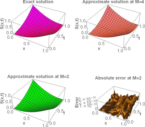
Figure 2. Absolute error graphical comparison of the present method solution, Legendre wavelet collocation method, and Chebyshev wavelet collocation method, for example, 1.

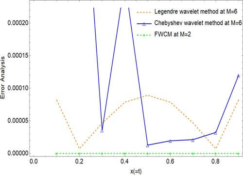
Figure 3. Graphical evaluation of the present method solution and the exact solution at different values of $x$, for example, 1.

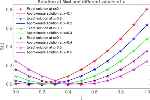
Figure 4. Graphical judgment between the proposed method solution and the exact solution at different values of $t$, for example, 1.

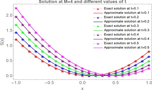
Table 1. Comparison of absolute errors by the FWCM, and different wavelet methods, for example, 1.

(x,t)	An absolute error by Legendre wavelet at $M=6$ [17]	An absolute error by the Chebyshev wavelet at $M=6$ [17]	An absolute error by FWCM at $M=2$	An absolute error by FWCM at $M=4$	An absolute error by FWCM at $M=6$
(0.1,0.1)	$8.20\times {10}^{-5}$	$4.16\times {10}^{-4}$	$3.46\times {10}^{-18}$	$5.48\times {10}^{-18}$	$1.92\times {10}^{-18}$
(0.2,0.2)	$7.10\times {10}^{-6}$	$5.37\times {10}^{-4}$	$1.38\times {10}^{-17}$	$1.50\times {10}^{-17}$	$1.19\times {10}^{-17}$
(0.3,0.3)	$4.65\times {10}^{-5}$	$3.55\times {10}^{-5}$	$2.77\times {10}^{-17}$	$1.36\times {10}^{-17}$	$3.22\times {10}^{-18}$
(0.4,0.4)	$7.86\times {10}^{-5}$	$2.65\times {10}^{-4}$	$5.55\times {10}^{-17}$	$2.68\times {10}^{-17}$	$3.74\times {10}^{-17}$
(0.5,0.5)	$8.93\times {10}^{-5}$	$1.27\times {10}^{-5}$	$5.55\times {10}^{-17}$	$4.19\times {10}^{-17}$	$1.02\times {10}^{-17}$
(0.6,0.6)	$7.86\times {10}^{-5}$	$1.93\times {10}^{-5}$	$1.11\times {10}^{-16}$	$3.86\times {10}^{-17}$	$6.61\times {10}^{-17}$
(0.7,0.7)	$4.65\times {10}^{-5}$	$2.11\times {10}^{-5}$	$1.11\times {10}^{-16}$	$4.87\times {10}^{-17}$	$1.36\times {10}^{-16}$
(0.8,0.8)	$7.10\times {10}^{-6}$	$3.22\times {10}^{-5}$	$2.22\times {10}^{-16}$	$1.64\times {10}^{-16}$	$1.53\times {10}^{-16}$
(0.9,0.9)	$8.22\times {10}^{-5}$	$1.20\times {10}^{-4}$	$2.22\times {10}^{-16}$	$1.36\times {10}^{-16}$	$7.99\times {10}^{-17}$

Table 2. Error norms comparison between the FWCM and other methods in the literature [17], for example, 1.

M	$L^2$ error via LW [17]	$L^2$ error via CW [17]	$L^{\mathrm{\infty }}$ error via LW [17]	$L^{\mathrm{\infty }}$ error via CW [17]	$L^2$ error via FWCM	$L^{\mathrm{\infty }}$ error via FWCM	RMS error via FWCM
2	$4.52\times {10}^{-1}$	$5.40\times {10}^{-1}$	$1.34\times {10}^{-1}$	$1.94\times {10}^{-1}$	$3.61\times {10}^{-16}$	$2.22\times {10}^{-16}$	$1.80\times {10}^{-16}$
4	$3.48\times {10}^{-4}$	$1.20\times {10}^{-3}$	$1.12\times {10}^{-4}$	$4.01\times {10}^{-4}$	$2.28\times {10}^{-16}$	$1.64\times {10}^{-16}$	$1.14\times {10}^{-16}$
6	$2.75\times {10}^{-4}$	$1.40\times {10}^{-3}$	$8.22\times {10}^{-4}$	$5.37\times {10}^{-4}$	$2.33\times {10}^{-16}$	$1.53\times {10}^{-16}$	$1.16\times {10}^{-16}$

Example 2. Consider another HPDE of first-order [16], $\begin{array}{rl}& {\displaystyle \frac{\mathrm{\partial }S\left(x,t\right)}{\mathrm{\partial }t}}+{\displaystyle \frac{\mathrm{\partial }S\left(x,t\right)}{\mathrm{\partial }x}}+S\left(x,t\right)\\ & =-2\sin \left(x+t\right)+\text{cos}\left(x+t\right),\\ & 0\le x\le 1,0\le t\le 1,\end{array}$ subject to the conditions: $\begin{array}{rl}S\left(x,0\right)& =\text{cos}\left(x\right),S\left(0,t\right)=\text{cos}\left(t\right),\\ & 0\le x\le 1,0\le t\le 1,\end{array}$

The exact solution is $S\left(x,t\right)=\text{cos}\left(x+t\right)$. This problem is solved by the projected technique. Figure 5 is a graphical representation of the current method solution at $M=3,6$ compared to the precise solution and its absolute error. Table 3 reveals that the absolute errors obtained from the proposed method are compared to those methods in the literature [16, 17, 20]. The absolute error graph of the present method and literature methods is drawn in Figure 6. From Tables 4 and 5 and Figures 6 and 7, we can see that the FWCM yields better results than the other literature methods [16, 18, 20]. Figures 8 and 9 reflect the graphical comparison of the FWCM solution with the exact solution at different values of $t$ and $x$, respectively.

Figure 5. Graphical illustration of FWCM and Exact solution along with its absolute error, for example, 2.

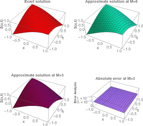
Figure 6. Graphical comparison of Shifted fifth-kind Chebyshev Galerkin method at $N=6$ (A1), Bernoulli matrix approach at $N=10$ (A2), Shifted Jacobi spectral-Galerkin method at $M=6$ (A3), present method at $M=3$ (A4), for example, 2.

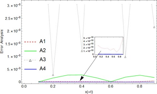
Figure 7. Graphical comparison of absolute errors of the present method and Shifted fifth-kind Chebyshev Galerkin method at $t=0.1$, for example, 2.

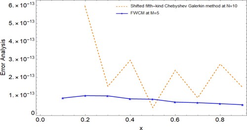
Figure 8. Graphical evaluation of the present method solution and the exact solution at different values of $t$, for example, 2.

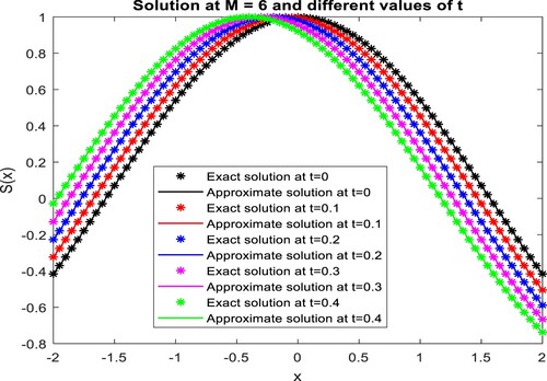
Figure 9. Graphical judgment of the present method solution and the exact solution at different values of $x$, for example, 2.

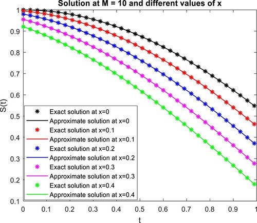
Table 3. Comparison of absolute errors by the projected method with the different literature methods, for example, 2.

(x,t)	An absolute error by Legendre wavelet at $M=6$ [17]	An absolute error by the Chebyshev wavelet at $M=6$ [17]	An absolute error by Shifted fifth-kind Chebyshev Galerkin method at $N=6$ [16]	An absolute error by the Bernoulli matrix approach at $N=10$ [20]	An absolute error by the Bernoulli matrix approach at $N=12$ [20]	An Absolute error by FWCM at $M=3$
(0.1,0.1)	$9.12\times {10}^{-5}$	$4.53\times {10}^{-4}$	$2.66\times {10}^{-10}$	$9.80\times {10}^{-11}$	$2.01\times {10}^{-11}$	$8.46\times {10}^{-12}$
(0.2,0.2)	$3.36\times {10}^{-5}$	$2.07\times {10}^{-4}$	$1.97\times {10}^{-10}$	$1.61\times {10}^{-9}$	$4.76\times {10}^{-12}$	$8.35\times {10}^{-12}$
(0.3,0.3)	$1.86\times {10}^{-5}$	$6.92\times {10}^{-5}$	$1.76\times {10}^{-10}$	$2.75\times {10}^{-9}$	$7.60\times {10}^{-11}$	$7.44\times {10}^{-12}$
(0.4,0.4)	$2.42\times {10}^{-5}$	$1.39\times {10}^{-4}$	$1.86\times {10}^{-10}$	$2.80\times {10}^{-9}$	$7.51\times {10}^{-11}$	$7.01\times {10}^{-12}$
(0.5,0.5)	$8.30\times {10}^{-5}$	$2.64\times {10}^{-5}$	$1.23\times {10}^{-10}$	$1.68\times {10}^{-9}$	$4.50\times {10}^{-11}$	$6.89\times {10}^{-12}$
(0.6,0.6)	$1.38\times {10}^{-4}$	$7.62\times {10}^{-5}$	$1.77\times {10}^{-10}$	$1.75\times {10}^{-10}$	$1.94\times {10}^{-12}$	$6.33\times {10}^{-12}$
(0.7,0.7)	$9.90\times {10}^{-5}$	$2.10\times {10}^{-5}$	$6.64\times {10}^{-11}$	$1.94\times {10}^{-9}$	$4.59\times {10}^{-11}$	$5.97\times {10}^{-12}$
(0.8,0.8)	$1.20\times {10}^{-6}$	$2.01\times {10}^{-5}$	$1.68\times {10}^{-10}$	$2.70\times {10}^{-9}$	$6.53\times {10}^{-11}$	$5.02\times {10}^{-12}$
(0.9,0.9)	$9.00\times {10}^{-5}$	$3.00\times {10}^{-4}$	$5.00\times {10}^{-10}$	$1.80\times {10}^{-9}$	$4.44\times {10}^{-11}$	$4.74\times {10}^{-12}$

Table 4. Comparison of absolute errors of the projected method and different literature methods, for example, 2.

	An absolute error by Shifted Jacobi spectral-Galerkin method at $M=6$ [18]
(x,t)	$\zeta =\eta =-{\displaystyle \frac{1}{2}}$	$\zeta =\eta =0$	$\zeta =\eta ={\displaystyle \frac{1}{2}}$	Absolute error at $M=3$ by FWCM
(0.1,0.1)	$5.51\times {10}^{-8}$	$8.41\times {10}^{-8}$	$1.03\times {10}^{-7}$	$8.46\times {10}^{-12}$
(0.2,0.2)	$5.33\times {10}^{-8}$	$2.84\times {10}^{-9}$	$4.98\times {10}^{-8}$	$8.35\times {10}^{-12}$
(0.3,0.3)	$1.05\times {10}^{-7}$	$6.39\times {10}^{-8}$	$2.41\times {10}^{-8}$	$7.44\times {10}^{-12}$
(0.4,0.4)	$3.62\times {10}^{-9}$	$1.22\times {10}^{-8}$	$2.85\times {10}^{-8}$	$7.01\times {10}^{-12}$
(0.5,0.5)	$1.30\times {10}^{-7}$	$1.10\times {10}^{-7}$	$1.04\times {10}^{-7}$	$6.89\times {10}^{-12}$
(0.6,0.6)	$1.28\times {10}^{-7}$	$9.93\times {10}^{-8}$	$8.85\times {10}^{-8}$	$6.33\times {10}^{-12}$
(0.7,0.7)	$3.53\times {10}^{-10}$	$9.84\times {10}^{-9}$	$4.72\times {10}^{-9}$	$5.97\times {10}^{-12}$
(0.8,0.8)	$1.02\times {10}^{-7}$	$7.22\times {10}^{-8}$	$3.72\times {10}^{-8}$	$5.02\times {10}^{-12}$
(0.9,0.9)	$3.75\times {10}^{-8}$	$2.16\times {10}^{-8}$	$6.65\times {10}^{-8}$	$4.74\times {10}^{-12}$

Table 5. Comparison of absolute errors of the projected method and method in literature at $t=0.1$, for example, 2.

x	An absolute error by Shifted fifth-kind Chebyshev Galerkin method at $N=10$ [16]	Absolute error at $M=5$ by FWCM
0.1	$1.10\times {10}^{-12}$	$8.46\times {10}^{-14}$
0.2	$5.87\times {10}^{-13}$	$9.81\times {10}^{-14}$
0.3	$1.50\times {10}^{-13}$	$9.66\times {10}^{-14}$
0.4	$2.95\times {10}^{-13}$	$8.01\times {10}^{-14}$
0.5	$3.13\times {10}^{-14}$	$7.81\times {10}^{-14}$
0.6	$2.39\times {10}^{-13}$	$6.20\times {10}^{-14}$
0.7	$8.62\times {10}^{-14}$	$5.87\times {10}^{-14}$
0.8	$2.74\times {10}^{-13}$	$5.32\times {10}^{-14}$
0.9	$1.43\times {10}^{-13}$	$4.72\times {10}^{-14}$

Example 3. Consider the linear HPDE of first-order [16], $\begin{array}{rl}& {\displaystyle \frac{\mathrm{\partial }S\left(x,t\right)}{\mathrm{\partial }t}}-{\displaystyle \frac{\mathrm{\partial }S\left(x,t\right)}{\mathrm{\partial }x}}-S\left(x,t\right)\\ & =-\sqrt{2}{e}^{-\sqrt{2}t-x},0\le x\le 1,0\le t\le 1,\end{array}$ subject to the conditions: $\begin{array}{rl}& S\left(x,0\right)=e^{-x},S\left(0,t\right)=e^{-\sqrt{2}t},\\ & 0\le x\le 1,0\le t\le 1,\end{array}$ The exact solution is $S\left(x,t\right)=e^{-\left(\sqrt{2}t+x\right)}$. We solved the above problem with the FWCM. Figure 10 is a surface plot of the FWCM at $M=6,9$ and the exact solution with its absolute error. Tables 6 and 7 show that the absolute error by the present method at $M=6andk=2$ is better than the methods in [16, 19]. Figures 11 and 12 show the graphical comparison of the current method solution at $M=6$ with the exact solution at different values of t and x, respectively.

Figure 10. Graphical illustration of FWCM and Exact solution along with the absolute error, for example, 3.

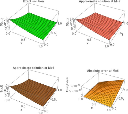
Figure 11. Graphical evaluation of the present method solution and the exact solution at different values of $x$, for example, 3.

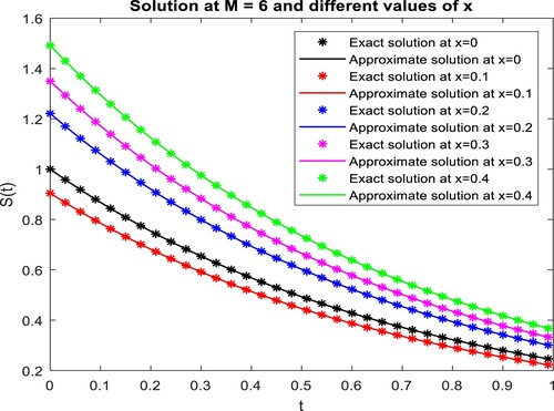
Figure 12. Graphical judgment of the present method solution and the exact solution at different values of $t,$ for example, 3.

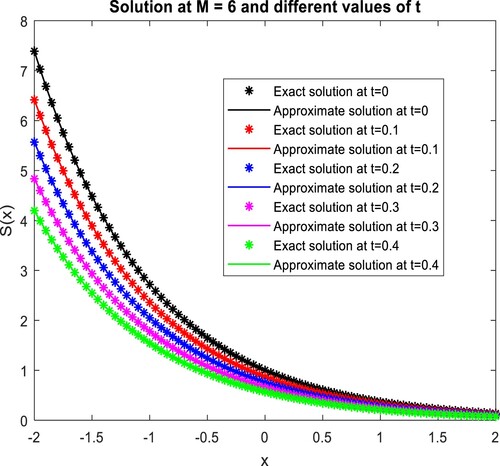
Table 6. Comparison of absolute errors of projected method and different collocation methods, for example, 3 at $t=0.1$.

x	An absolute error by Shifted fifth-kind Chebyshev Galerkin method at $N=10$ [16]	Generalized Laguerre-Gauss-Radau collocation scheme $N=M=16$ [19]	An absolute error by FWCM at $M=6$ and $k=2$
0.1	$3.52\times {10}^{-14}$	$2.84\times {10}^{-7}$	9.34$\times {10}^{-17}$
0.2	$9.87\times {10}^{-15}$	$8.79\times {10}^{-6}$	8.65$\times {10}^{-17}$
0.3	$5.89\times {10}^{-16}$	$1.20\times {10}^{-5}$	6.87$\times {10}^{-17}$
0.4	$2.24\times {10}^{-14}$	$1.12\times {10}^{-5}$	4.01$\times {10}^{-17}$
0.5	$1.70\times {10}^{-14}$	$7.95\times {10}^{-6}$	1.77$\times {10}^{-17}$
0.6	$2.85\times {10}^{-14}$	$3.29\times {10}^{-6}$	8.74$\times {10}^{-16}$
0.7	$1.23\times {10}^{-15}$	$1.78\times {10}^{-6}$	6.55$\times {10}^{-16}$
0.8	$6.58\times {10}^{-14}$	$6.53\times {10}^{-6}$	4.32$\times {10}^{-16}$
0.9	$2.23\times {10}^{-12}$	$1.04\times {10}^{-5}$	7.25$\times {10}^{-15}$

Table 7. Comparison of absolute errors of projected method and different collocation methods, for example, 3 at $t=0.5$.

x	An absolute error by Shifted fifth-kind Chebyshev Galerkin method at $N=10$ [16]	Generalized Laguerre-Gauss-Radau collocation scheme $N=M=16$ [19]	An absolute error by FWCM at $M=6$ and $k=2$
0.1	$2.59\times {10}^{-14}$	$8.95\times {10}^{-6}$	8.56$\times {10}^{-17}$
0.2	$4.25\times {10}^{-14}$	$4.10\times {10}^{-6}$	7.33$\times {10}^{-17}$
0.3	$1.55\times {10}^{-15}$	$1.39\times {10}^{-5}$	5.46$\times {10}^{-17}$
0.4	$9.83\times {10}^{-14}$	$2.07\times {10}^{-5}$	3.21$\times {10}^{-17}$
0.5	$3.33\times {10}^{-12}$	$2.47\times {10}^{-5}$	2.27$\times {10}^{-17}$
0.6	$5.37\times {10}^{-11}$	$2.62\times {10}^{-5}$	9.03$\times {10}^{-16}$
0.7	$3.71\times {10}^{-10}$	$2.55\times {10}^{-5}$	$7.65\times {10}^{-16}$
0.8	$1.72\times {10}^{-9}$	$2.31\times {10}^{-5}$	$5.11\times {10}^{-16}$
0.9	$6.26\times {10}^{-9}$	$1.93\times {10}^{-5}$	$3.49\times {10}^{-15}$

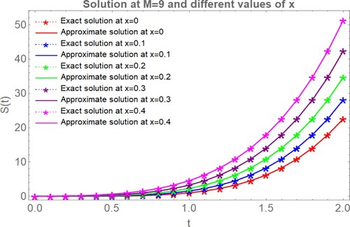
Example 4. Consider one more HPDE of first-order [16], $\begin{array}{rl}& {\displaystyle \frac{\mathrm{\partial }S\left(x,t\right)}{\mathrm{\partial }t}}-{\displaystyle \frac{\mathrm{\partial }S\left(x,t\right)}{\mathrm{\partial }x}}-S\left(x,t\right)\\ & =e^{-t-x}\left(\cos \left(t\right)-sin\left(t\right)\right),0\le x\le 1,0\le t\le 1,\end{array}$ subject to the conditions: $S\left(x,0\right)=0,S\left(0,t\right)=e^{-t}sin\left(t\right),0\le x\le 1,0\le t\le 1,$

The exact solution is $S\left(x,t\right)=e^{-\left(t+x\right)}sin\left(t\right)$. The graphical presentation of the current technique solution compared with the exact solution in Figure 13. Figures 14 and 15 explain the graphical evaluation of the FWCM solution at $M=9$ with the exact solution at different values of x and t, respectively. Tables 8 and 9 represent that for the small value of M and k, we obtained a higher accuracy in the solution than the method in [18]. Also, k and M values are directly proportional to the closeness of the solution.

Figure 13. Graphical illustration of FWCM and Exact solution along with the absolute error, for example, 4.

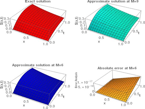
Figure 14. Graphical evaluation of the present method solution and the exact solution at different values of $t,$ for example, 4.

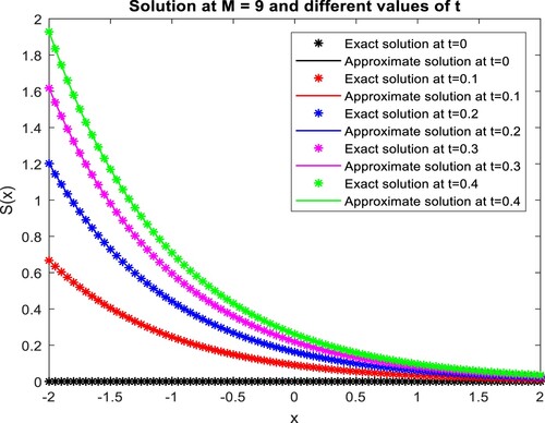
Figure 15. Graphical judgment of the present method solution and the exact solution at different values of $x,$ for example, 4.

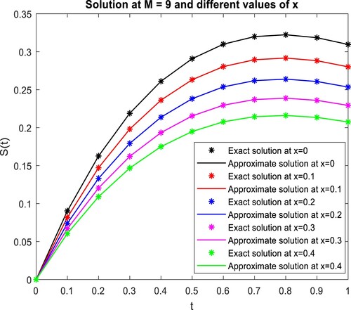
Table 8. Comparison of absolute errors of projected method and different collocation method, for example, 4 at $t=0.1$.

	An absolute error by Shifted Jacobi spectral-Galerkin method [18]
x	$\zeta =\eta =-{\displaystyle \frac{1}{2}}$	$\zeta =\eta =-{\displaystyle \frac{1}{2}}$	An absolute error by FWCM at $M=9$ and $k=1$	An absolute error by FWCM at $M=6$ and $k=2$
0.1	$3.64\times {10}^{-17}$	$3.59\times {10}^{-16}$	8.41$\times {10}^{-17}$	9.52$\times {10}^{-18}$
0.2	$1.38\times {10}^{-15}$	$8.81\times {10}^{-16}$	8.02$\times {10}^{-17}$	8.34$\times {10}^{-18}$
0.3	$1.03\times {10}^{-15}$	$1.38\times {10}^{-15}$	7.55$\times {10}^{-17}$	6.40$\times {10}^{-18}$
0.4	$1.15\times {10}^{-15}$	$1.29\times {10}^{-15}$	6.93$\times {10}^{-17}$	5.07$\times {10}^{-18}$
0.5	$1.08\times {10}^{-15}$	$1.31\times {10}^{-15}$	5.32$\times {10}^{-17}$	3.86$\times {10}^{-18}$
0.6	$1.54\times {10}^{-15}$	$1.67\times {10}^{-15}$	4.99$\times {10}^{-17}$	2.24$\times {10}^{-18}$
0.7	$1.41\times {10}^{-15}$	$1.81\times {10}^{-15}$	4.08$\times {10}^{-17}$	9.04$\times {10}^{-17}$
0.8	$1.12\times {10}^{-15}$	$1.96\times {10}^{-15}$	2.81$\times {10}^{-17}$	7.66$\times {10}^{-17}$
0.9	$1.13\times {10}^{-15}$	$1.92\times {10}^{-15}$	9.68$\times {10}^{-16}$	6.37$\times {10}^{-17}$
1.0	$6.38\times {10}^{-16}$	$9.71\times {10}^{-16}$	7.33$\times {10}^{-16}$	4.21$\times {10}^{-17}$

Table 9. Comparison of absolute errors of projected method and different collocation method, for example, 4 at $t=0.5$.

	An absolute error by Shifted Jacobi spectral-Galerkin method [18]
X	$\zeta =\eta =-{\displaystyle \frac{1}{2}}$	$\zeta =\eta =-{\displaystyle \frac{1}{2}}$	An absolute error by FWCM at $M=9$ and $k=1$	An absolute error by FWCM at $M=6$ and $k=2$
0.1	$3.22\times {10}^{-16}$	$2.28\times {10}^{-16}$	$6.34\times {10}^{-17}$	$5.14\times {10}^{-18}$
0.2	$4.30\times {10}^{-16}$	$2.56\times {10}^{-16}$	$5.97\times {10}^{-17}$	$5.09\times {10}^{-18}$
0.3	$1.05\times {10}^{-15}$	$1.11\times {10}^{-16}$	$5.14\times {10}^{-17}$	$4.33\times {10}^{-18}$
0.4	$9.99\times {10}^{-16}$	$1.11\times {10}^{-16}$	$4.28\times {10}^{-17}$	$3.54\times {10}^{-18}$
0.5	$1.15\times {10}^{-15}$	$1.66\times {10}^{-16}$	$3.87\times {10}^{-17}$	$2.99\times {10}^{-18}$
0.6	$1.94\times {10}^{-16}$	$5.55\times {10}^{-16}$	$2.45\times {10}^{-17}$	$1.05\times {10}^{-18}$
0.7	$1.66\times {10}^{-16}$	$8.04\times {10}^{-16}$	$1.70\times {10}^{-17}$	$8.22\times {10}^{-17}$
0.8	$1.69\times {10}^{-15}$	$1.02\times {10}^{-15}$	$8.66\times {10}^{-16}$	$6.79\times {10}^{-17}$
0.9	$1.63\times {10}^{-15}$	$1.22\times {10}^{-15}$	$7.42\times {10}^{-16}$	$5.66\times {10}^{-17}$
1.0	$1.49\times {10}^{-15}$	$9.99\times {10}^{-16}$	$5.24\times {10}^{-16}$	$3.04\times {10}^{-17}$

Notes: Fractional-order integro-differential equations using Laguerre wavelet method, Journal of Information.

Example 5. Consider the linear hyperbolic equation of first-order [16], $\begin{array}{rl}& {\displaystyle \frac{\mathrm{\partial }S\left(x,t\right)}{\mathrm{\partial }t}}+{\displaystyle \frac{\mathrm{\partial }S\left(x,t\right)}{\mathrm{\partial }x}}+S\left(x,t\right)\\ & =(x+t{)}^{\frac{7}{2}}\left(x+t+9\right),0\le x\le 1,0\le t\le 1,\end{array}$ subject to the conditions: $S\left(x,0\right)=(x{)}^{\frac{9}{2}},S\left(0,t\right)=(t{)}^{\frac{9}{2}},0\le x\le 1,0\le t\le 1,$ The exact solution is $S\left(x,t\right)=(x+t{)}^{\frac{9}{2}}$. The projected technique FWCM solves this problem. The graphical presentation of the present approach solution at $M=6,9$ compared with the exact solution is shown in Figure 16, and the error graph is also drawn. Figure 17 and Figure 18 explain the graphical judgment of the FWCM solution at $M=9$ with the exact solution at different values of x and t.

Figure 16. Graphical illustration of FWCM and Exact solution along with the absolute error, for example, 5.

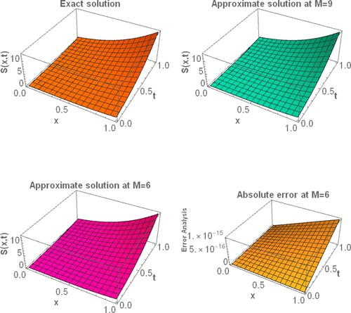
Figure 17. Graphical evaluation of the present method solution and the exact solution at different values of $t,$ for example, 5.

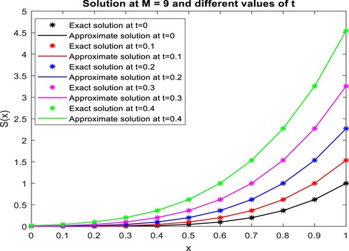
Figure 18. Graphical judgment of the present method solution and the exact solution at different values of $x,$ for example, 5.

6. Conclusion

This article introduced the Fibonacci wavelet operational matrix of integration through the linear combination concepts. Based on this Fibonacci wavelets matrix, we have projected an efficient algorithm for solving hyperbolic partial differential equations with the help of the Mathematica software. In this approach, first given HPDEs are transformed into a system of algebraic equations then the solution will be obtained with the help of the Newton–Raphson method. The efficiency of the proposed method can be seen in the tables and graphs. Also, the current approach is better than the methods in [16-20]. The projected method takes less computational time and achieves excellent precision at less resolution level. Table 1 shows that by increasing the $\text{M}$ values simultaneously accuracy in the solution also increases. Tables 8 and 9 reveal that on varying $\text{k}$ values we get still higher accuracy in the solution.

Acknowledgments

The authors are grateful to the referees and the editor for carefully checking the details and for helpful comments that improved this paper. Also, the author thanks to Backward Classes Welfare Department, Karnataka for the Ph.D. fellowship.

Disclosure statement

No potential conflict of interest was reported by the author(s).

Data availability statement

The data that support the findings of this study are available within the article.

References

- Strub I, Bayen A. Optimal control of air traffic networks using continuous flow model. (AIAA Conference on Guidance, Control, and Dynamics, Keystone, Colorado). 2006;3:1700–1710.
- Bendahmane M, Nagaiah C, Comte É, et al. A 3D boundary optimal control for the bidomain-bath system modeling the thoracic shock therapy for cardiac defibrillation. J Math Anal Appl. 2016;437(2). hal-01261547.
- Ng KW, Rohanin A. Numerical solution for PDE-constrained optimization problem in cardiac electrophysiology. Int J Comput Appl. 2012;44(12):11–15.
- Martínez A, Rodríguez C, Vázquez M. Theoretical and numerical analysis of an optimal control problem related to wastewater treatment. SIAM J Control Optim. 2000;38(5):1534–1553.
- Maidi A, Corriou J. Optimal control of nonlinear chemical processes using the variational iteration method. IFAC Symposium Advanced Control of Chemical Processes. 2012;45(15):898–903.
- Bhatti MM, Zeeshan A, Bashir F, et al. Sinusoidal motion of small particles through a Darcy-Brinkman-Forchheimer microchannel filled with non-Newtonian fluid under electro-osmotic forces. J Taibah Univ Sci. 2021;15(1):514–529.
- Tereshko D. Discrete optimization of unsteady fluid flows. CEUR Workshop Proc. 2016;1623:293–302.
- Sadiya U, Inc M, Arefin MA, et al. Consistent travelling waves solutions to the non-linear time fractional Klein–Gordon and Sine-Gordon equations through extended tanh-function approach. J Taibah Univ Sci. 2022;16(1):594–607.
- Munteanu I, Bratcu A, Cutululis N, et al. Optimal control of wind energy systems towards a global approach. Adv Ind Control. 2008.
- Lenhart S, Workman JT. Optimal control applied to biological model. Math Comput Biol. 2007.
- Gökmen E. A computational approach with residual error analysis for the fractional-order biological population model. J Taibah Univ Sci. 2021;15(1):218–225.
- Gibson WC. The method of moments in electromagnetics. Abingdon: Taylor and Francis Group; 2008.
- Pettersson MP, Iaccarino G, Nordström J. Polynomial chaos methods for hyperbolic partial differential equations: numerical techniques for fluid dynamics problems in the presence of uncertainties. Cham: Springer International Publishing; 2015.
- Yeh KC, Liu CH. Wave propagation in random media in theory of ionospheric waves. Cambridge (MA): Academic Press. 1972;17:308–366.
- Vergara RC. Development of geostatistical models using stochastic partial differential equations [Ph.D. thesis]. Paris: Université Paris Sciences et Lettres; 2018.
- Atta AG, Abd-Elhameed WM, Moatimid GM, et al. Shifted fifth-kind Chebyshev Galerkin treatment for linear hyperbolic first-order partial differential equations. Appl Numer Math. 2021;167:237–256.
- Singh S, Patel VK, Singh VK. Application of wavelet collocation method for hyperbolic partial differential equations via matrices. Appl Math Comput. 2018;320:407–424.
- Doha EH, Hafez RM, Youssri YH. Shifted Jacobi spectral-Galerkin method for solving hyperbolic partial differential equations. Comp Math Appl. 2019;78:889–904.
- Bhrawy AH, Hafez RM, Alzahrani EO, et al. Generalized Laguerre-Gauss-Radau scheme for the first order hyperbolic equations in a semi-infinite domain. Rom J Phys. 2015;60(7-8):918–934.
- Tohidi E, Toutounian F. Convergence analysis of Bernoulli matrix approach for one-dimensional matrix hyperbolic equations of the first order. Comput Math Appl. 2014;68(1-2):1–12.
- Shiralashetti SC, Kumbinarasaiah S. Laguerre wavelets collocation method for the numerical solution of the Benjamina–Bona–Mohany equations. J Taibah Univ Sci. 2019;13(1):9–15.
- Shahni J, Singh R. Numerical simulation of Emden–Fowler integral equation with Green’s function type kernel by Gegenbauer-wavelet, Taylor-wavelet, and Laguerre-wavelet collocation methods. Math Comput Simul. 2022;194:430–444.
- Shahni J, Singh R. Laguerre wavelet method for solving Thomas–Fermi type equations. Eng Comput. 2022;38:2925–2935.
- Behera S, Ray SS. On a wavelet-based numerical method for linear and nonlinear fractional Volterra integro-differential equations with weakly singular kernels. Comput Appl Math. 2022;41:211.
- Guo L, Yu Z. A Gaussian wavelet-based method for extracting rockfall motion information in consecutive impact tests on flexible barrier systems. Int J Impact Eng. 2022;167:104264.
- Gupta S, Ranta S. Legendre wavelet based numerical approach for solving a fractional eigenvalue problem. Chaos, Solitons Fractals. 2022;155:111647.
- Kumbinarasaiah S, Raghunatha KR. Numerical solution of the Jeffery–Hamel flow through the wavelet technique. Heat Transfer. 2022;51:1568–1584.
- Saeed U, Rehman MU. Hermite wavelet method for fractional delay differential equations. J Diff Equ. 2014;2014:359093.
- Kumbinarasaiah S. A novel approach for multi-dimensional fractional coupled Navier–Stokes equation. SeMA; 2022.
- Sezen C, Partal T. New hybrid GR6J-wavelet-based genetic algorithm-artificial neural network (GR6J-WGANN) conceptual-data-driven model approaches for daily rainfall–runoff modelling. Neural Comput Appl. 2022;34:17231–17255.
- Janjarasjitt S. Comparison of wavelet-based decomposition and empirical mode decomposition of electrogastrogram signals for preterm birth classification. ETRI J. 2022: 1–11.
- Adebayo TS. Environmental consequences of fossil fuel in Spain amidst renewable energy consumption: new insights from the wavelet-based Granger causality approach. Int J Sustain Dev World Ecol. 2022.
- Ahsan M, Hussain I, Ahmad M. A finite-difference and Haar wavelets hybrid collocation technique for non-linear inverse Cauchy problems. Appl Math Sci Eng. 2022;30(1):121–140.
- El-Gamel M, Mohamed N, Adel W. Numerical study of a nonlinear high order boundary value problems using Genocchi collocation technique. Int J Appl Comput Math. 2022;8:143.
- Liu C, Yu Z, Zhang X, et al. An implicit wavelet collocation method for variable coefficients space fractional advection-diffusion equations. Appl Numer Math. 2022;177:93–110.
- Sabermahani S, Ordokhani Y, Yousefi S. Fibonacci wavelets and their applications for solving two classes of time-varying delay problems. Optim Control Appl Methods. 2020;41:395–416.
- Shah FA, Irfan M, Nisar KS, et al. Fibonacci wavelet method for solving time-fractional telegraph equations with Dirichlet boundary conditions. Results Phys. 2021;24:104123.
- Shiralashetti SC, Lamani L. Fibonacci wavelet based numerical method for the solution of nonlinear Stratonovich Volterra integral equations. Sci Afr. 2020;10:e00594.
- Mohd I, Shah FA, Nisar KS. Fibonacci wavelet method for solving Pennes bioheat transfer equation. Int J Wavelets Multiresolut Inf Process. 2021;19(6):2150023.
- Sabermahani S, Ordokhani Y. Fibonacci wavelets and Galerkin method to investigate fractional optimal control problems with bibliometric analysis. J Vib Control. 2021;27(15-16):1778–1792.
- Kurt A, Yalçınbaş S, Sezer M. Fibonacci collocation method for solving high-order linear Fredholm integro-differential-difference equations. Int J Math Math Sci. 2013;2013:486013.
- Alkan S, Cakmak M. Fibonacci collocation method for solving a class of systems of nonlinear differential equations. New Trends Math Sci. 2021;9(4):11–24.
- Shiralashetti SC, Lamani L. A modern approach for solving nonlinear Volterra integral equations using Fibonacci wavelets. Electron J Math Anal Appl. 2021;9(2):88–98.
- Irfan M, Shah FA. Fibonacci wavelet method for solving the time-fractional bioheat transfer model. Optik (Stuttg). 2021;241:167084.