Phase characterization and exraction of new forms of solitons for the (3+1)-dimensional q-deformed Sinh-Gordon equation

Abstract

In this article, the (3+1)-dimensional q-deformed Sinh-Gordon model is investigated to extract analytical solutions using the unified method. This technique effectively extracts polynomial and rational function solutions. When the appropriate limiting constraints are given to the parameters, this technique successfully retrieves hyperbolic and trigonometric results. Some graphical representations of the solutions of the proposed equation are illustrated. Additionally, all feasible phase portraits are shown, the planer dynamical system of the equation under discussion is built using Galilean transformation, and sensitive inspection is used to verify the sensitivity of the equation under consideration. There aren't many previous methods for solving this kind of equation, either analytically or numerically. This work is highly valuable for the understanding of various symmetrical physical systems.

Keywords:

• q-deformed Sinh-Gordon equation
• travelling wave transformation
• unified method
• soliton
• quantitative analysis

1. Introduction

The study of optical solitons has gathered a great deal of interest and is currently one of the most hot topics of research. This topic plays an important role in describing some phenomena in science, engineering, and technology, including quantum optics [1], optical communications [2], nonlinear dynamics [3] and plasma physics [4]. Solitary wave (soliton) propagation is one of the most important phenomena that many researchers have been looking for to analyse and comprehend. The solitons have a specific direction on how to develop and spread the information. This form of wave is very common in nature, and it has a lot of applications in optical fibres [5]. The concept of soliton is defined as the wave packet that keeps its shape while it travels at a steady speed.

A delicate balance between dispersion and nonlinearity can be used to describe this property. The soliton solution plays a vital role in integrable models. Solitons are produced by a variety of famous nonlinear PDEs, including Sawada-Kotera equations [6,7], Biswas-Milovic equations [8], Schrödinger equations [9], coupled KDV equations [10] and BKP equations [11].

Non-linear evolution equations (NLEEs) are now used to illustrate complex physical processes in several areas of research, including physics [12], chemistry [13], biology [14] and engineering [15]. Numerous schemes for extracting exact and numerical solutions for nonlinear evolution equations (NLEEs) are developed to obtain necessary information for understanding real problems in a variety of engineering fields and science, such as the G'/G expansion method for exploring exact solitary wave solutions [16], Wronskian formulation [17], Painlevé approach [18], the Hirota bilinear method [19], linear superposition principle [20], inverse scattering method [21] and the invariant method [22].

In recent years, substantial progress has been achieved, and a number of reliable and efficient methodologies for retrieving accurate NLEE solutions have been devised [23–28]. The Sinh-Gordon equation has been studied using self-similar transformaion[29], the analytic solutions have been extracted applying similarity transformation and Hirota's bilinear method [30]. Moreover, the two-soliton solution for this model has been investigated in the literature [31]. While the under consideration model and several methods of solving it were well-known in the 19th century, its significance increased notably when it was discovered that the resulting solution contributes to the colliding features of solitons (kink and antikink). Other practical implications of the Sinh-Gordon equation include the movement of a suspended pendulum tied to a stretched wire, the transmission of flux in Josephson junctions (a connection between two superconductors) and displacements in crystals. The governing problem is investigated using the unified approach [32], one of the most evident, clear, and effective mathematical techniques for obtaining accurate answers. Because it delivers exact solutions in the form of polynomial and rational functions, the applied technique is helpful and efficient. Different wave solutions are represented by polynomial solutions, whereas periodic and soliton forms are described by rational function solutions. Moreover, the bifurcation of the dynamical system of the stated equation is also studied. Using a bifurcation analysis of the planner dynamical system [33–35], all possibilities for parameter dependency have been examined to see the geometrical properties of the discussed model.

The rest of the article is organized as follows: The governing model is discussed in Section 2. The principles of mathematical analysis are covered in Section 3. Section 4 gives an insight into the technique in concern. The proposed procedure is discussed in Section 5, which explains how to generate soliton solutions. The derived solutions to the governing problems are graphically represented in Section 6. The qualitative analysis is detailed in Section 7. Finally, the work's conclusion is offered in Section 8.

2. Governing model

The generalized (3+1) dimensional q-deformed Sinh-Gordon equation [36,37] (3+1)-dimensional Eleuch equation) is the subject of this paper, described as (1) $(\frac{{\mathrm{\partial }}^2}{\mathrm{\partial }{x}^2}+\frac{{\mathrm{\partial }}^2}{\mathrm{\partial }{y}^2}+\frac{{\mathrm{\partial }}^2}{\mathrm{\partial }{z}^2}-\frac{{\mathrm{\partial }}^2}{\mathrm{\partial }{t}^2})u={[{\sinh }_q(u^{\gamma })]}^p-\delta ,$(1) Which can be written as (2) $\mathrm{◻u}=(\mathrm{\Delta }-\frac{{\mathrm{\partial }}^2}{\mathrm{\partial }{t}^2})u={[{\sinh }_q(u^{\gamma })]}^p-\delta ,$(2) where $◻$ is the d'Alembert operator where ${\sinh }_q$ represents the function of q-deformed characterized by (3) ${\sinh }_q(z)=\frac{e^z-q{e}^{-z}}{2}\text{where}0<q\le 1.$(3) With q = 1, conventional sinh functions are provided. ${\cosh }_q(z)$, ${\tanh }_q(z)$ and their reciprocal are explained in [36]. The offered methodology will be used to investigate the optical soliton related to Equation (8(8) $B(z,t,b_x,b_t,b_{\mathrm{xt}},b_{2x},b_{2\mathrm{xt}}\cdots ,b_{\mathrm{cxt}})=0;c\ge 0,$(8) ).

3. The mathematical examination

To solve Equation (1(1) $(\frac{{\mathrm{\partial }}^2}{\mathrm{\partial }{x}^2}+\frac{{\mathrm{\partial }}^2}{\mathrm{\partial }{y}^2}+\frac{{\mathrm{\partial }}^2}{\mathrm{\partial }{z}^2}-\frac{{\mathrm{\partial }}^2}{\mathrm{\partial }{t}^2})u={[{\sinh }_q(u^{\gamma })]}^p-\delta ,$(1) ) for travelling wave solutions consider the transformation [38] as (4) $\xi =\frac{(x+y+z)-\mathrm{\beta t}}{\sqrt{1-{\beta }^2}};$(4) where the velocity of travelling wave is denoted by β. Equation (1(1) $(\frac{{\mathrm{\partial }}^2}{\mathrm{\partial }{x}^2}+\frac{{\mathrm{\partial }}^2}{\mathrm{\partial }{y}^2}+\frac{{\mathrm{\partial }}^2}{\mathrm{\partial }{z}^2}-\frac{{\mathrm{\partial }}^2}{\mathrm{\partial }{t}^2})u={[{\sinh }_q(u^{\gamma })]}^p-\delta ,$(1) ) has taken the form of following ODE, using Equation (4(4) $\xi =\frac{(x+y+z)-\mathrm{\beta t}}{\sqrt{1-{\beta }^2}};$(4) ) (5) $\frac{d^{2}y(\xi )}{d{\xi }^2}={[{\sinh }_q(y^{\gamma }(\xi ))]}^p-\delta .$(5) For this article, For p = 1, $\gamma =1$ and $\delta =0$, the aforementioned equation is investigated. In the next section, the travelling wave solutions for Equation (5(5) $\frac{d^{2}y(\xi )}{d{\xi }^2}={[{\sinh }_q(y^{\gamma }(\xi ))]}^p-\delta .$(5) ) were derived using a recommended analytical method by applying the transformation given below. (6) $f(\gamma )=e^{y(\gamma )}.$(6) Using Equation (6(6) $f(\gamma )=e^{y(\gamma )}.$(6) ), Equation (5(5) $\frac{d^{2}y(\xi )}{d{\xi }^2}={[{\sinh }_q(y^{\gamma }(\xi ))]}^p-\delta .$(5) ) becomes (7) $-2f^{\prime 2}+2f{f}^{″}-f^3+\mathrm{qf}=0.$(7)

4. Overview of the proposed method

Unified technique:

Let the structure of q-deformed model be expressed like (8) $B(z,t,b_x,b_t,b_{\mathrm{xt}},b_{2x},b_{2\mathrm{xt}}\cdots ,b_{\mathrm{cxt}})=0;c\ge 0,$(8) here B stands for the function. It is possible to change the pattern $\nu =\mathrm{\beta z}-\mathrm{wt}$ using the travelling wave parameter (9) $B(b,b^{\mathrm{\prime }},b^{\mathrm{\prime \prime }},\dots ,b^c)=0,$(9) here $b^{\mathrm{\prime }}$ presents the differentiation for b including a new parameter ν. To extract the solution for (9(9) $B(b,b^{\mathrm{\prime }},b^{\mathrm{\prime \prime }},\dots ,b^c)=0,$(9) ), the UM technique has been used to find rational or polynomial function solutions. We are going to consider the polynomial function solution. The method is discussed below:

Polynomial form:

(9(9) $B(b,b^{\mathrm{\prime }},b^{\mathrm{\prime \prime }},\dots ,b^c)=0,$(9) ) has a solution in polynomial form like (10) $Q(\mu )=\sum _{n=0}^m{r}_i{\mathrm{{\rm Y}}}^i(\mu ).r_n\ne 0,$(10) $r_i$ are constants. The function $\mathrm{{\rm Y}}(\mu )$ will be found by considering the auxiliary equation: (11) ${({\mathrm{{\rm Y}}}^{\mathrm{\prime }}(\mu ))}^{\sigma }=\sum _{n=0}^{\mathrm{\sigma j}}{c}_i{\mathrm{{\rm Y}}}^i(\nu ),\sigma =1,2,$(11) where $c_i$ are parameters. Moreover, it's important to look out for numerical values related to n as examined in terms related to j by substituting the homogenous conditions among the highest derivatives along with highest nonlinear terms involved in (9(9) $B(b,b^{\mathrm{\prime }},b^{\mathrm{\prime \prime }},\dots ,b^c)=0,$(9) ), whereas j is revealed by utilizing the consistency condition.

where to solve (10(10) $Q(\mu )=\sum _{n=0}^m{r}_i{\mathrm{{\rm Y}}}^i(\mu ).r_n\ne 0,$(10) ), the Unified Method deals with (10(10) $Q(\mu )=\sum _{n=0}^m{r}_i{\mathrm{{\rm Y}}}^i(\mu ).r_n\ne 0,$(10) ) for the elliptic or elementary solution when $\sigma =1$ and $\sigma =2$.

Rational form:

The basic part of the presented portion is to let (9(9) $B(b,b^{\mathrm{\prime }},b^{\mathrm{\prime \prime }},\dots ,b^c)=0,$(9) ) has the following solution (12) $Q(\nu )=\frac{\sum _{m=0}^n{b}_m{\mathrm{{\rm Y}}}^m(\nu )}{\sum _{m=0}^r{q}_m{\mathrm{{\rm Y}}}^m(\nu )},n\ge r,$(12) with an auxiliary model (13) $({\mathrm{{\rm Y}}}^{\mathrm{\prime }}(\nu ){)}^{\sigma }=\sum _{i=0}^{\mathrm{\sigma v}}{\beta }_i{\mathrm{{\rm Y}}}^i(\nu ),\sigma =1,2.$(13) In  (12(12) $Q(\nu )=\frac{\sum _{m=0}^n{b}_m{\mathrm{{\rm Y}}}^m(\nu )}{\sum _{m=0}^r{q}_m{\mathrm{{\rm Y}}}^m(\nu )},n\ge r,$(12) ) and (13(13) $({\mathrm{{\rm Y}}}^{\mathrm{\prime }}(\nu ){)}^{\sigma }=\sum _{i=0}^{\mathrm{\sigma v}}{\beta }_i{\mathrm{{\rm Y}}}^i(\nu ),\sigma =1,2.$(13) ), $b_m$, $q_m$ and ${\beta }_i$ are unspecified parameters to be relieved, in such technique, the solution formed through (12(12) $Q(\nu )=\frac{\sum _{m=0}^n{b}_m{\mathrm{{\rm Y}}}^m(\nu )}{\sum _{m=0}^r{q}_m{\mathrm{{\rm Y}}}^m(\nu )},n\ge r,$(12) ) fulfils  (9(9) $B(b,b^{\mathrm{\prime }},b^{\mathrm{\prime \prime }},\dots ,b^c)=0,$(9) ). It's vital for looking out numerical interpretations of n, v are exerted employing balancing criteria using the highest order for linear or nonlinear terms in (9(9) $B(b,b^{\mathrm{\prime }},b^{\mathrm{\prime \prime }},\dots ,b^c)=0,$(9) ). By applying the consistency criteria, we could found unknown constants among (12(12) $Q(\nu )=\frac{\sum _{m=0}^n{b}_m{\mathrm{{\rm Y}}}^m(\nu )}{\sum _{m=0}^r{q}_m{\mathrm{{\rm Y}}}^m(\nu )},n\ge r,$(12) ). The UM technique will be employed for solving (12(12) $Q(\nu )=\frac{\sum _{m=0}^n{b}_m{\mathrm{{\rm Y}}}^m(\nu )}{\sum _{m=0}^r{q}_m{\mathrm{{\rm Y}}}^m(\nu )},n\ge r,$(12) ). After that, we got a solution for $\sigma =1$ or $\sigma =2$, respectively.

5. Extraction of soliton

This portion deals with the exploration of solutions concerning the governing Equation (1(1) $(\frac{{\mathrm{\partial }}^2}{\mathrm{\partial }{x}^2}+\frac{{\mathrm{\partial }}^2}{\mathrm{\partial }{y}^2}+\frac{{\mathrm{\partial }}^2}{\mathrm{\partial }{z}^2}-\frac{{\mathrm{\partial }}^2}{\mathrm{\partial }{t}^2})u={[{\sinh }_q(u^{\gamma })]}^p-\delta ,$(1) ) with the help of the proposed technique.

5.1. Exact solution using a unified method

Equation (7(7) $-2f^{\prime 2}+2f{f}^{″}-f^3+\mathrm{qf}=0.$(7) ) is investigated using a unified approach to retrieve soliton solutions as described below.

Balancing $f^{\prime 2}$ and $f^3$ in Equation (7(7) $-2f^{\prime 2}+2f{f}^{″}-f^3+\mathrm{qf}=0.$(7) ) produces balancing number 2. The suggested solution is as follows: (14) $f(\xi )=\sum _{i=0}^1{r}_i{\chi }^i(\xi ),r_1\ne 0,$(14) with the auxiliary equation (15) ${\left(\mathrm{{\rm Y}}{}^{\prime }\left(\xi \right)\right)}^{\sigma }=\sum _{p=0}^{2\sigma }{c}_i{\mathrm{{\rm Y}}}^i(\xi ),\sigma =1;2.$(15)

5.1.1. Solitary wave solution

Here, we'll retrieve the solitary solution regarding Equation (7(7) $-2f^{\prime 2}+2f{f}^{″}-f^3+\mathrm{qf}=0.$(7) ).

For this reason, we should substitute $\sigma =1$ in the auxiliary Equation (15(15) ${\left(\mathrm{{\rm Y}}{}^{\prime }\left(\xi \right)\right)}^{\sigma }=\sum _{p=0}^{2\sigma }{c}_i{\mathrm{{\rm Y}}}^i(\xi ),\sigma =1;2.$(15) ) ;therefore, we obtained (16) $\begin{array}{rl}Q(\xi )& =r_0+r_1\mathrm{{\rm Y}}\left(\xi \right)+r_2\mathrm{{\rm Y}}{\left(\xi \right)}^2,\\ {\mathrm{{\rm Y}}}^{\mathrm{\prime }}(\xi )& =c_0+c_1\mathrm{{\rm Y}}\left(\xi \right)+c_2{\mathrm{{\rm Y}}}^2\left(\xi \right).\end{array}$(16) The system of nonlinear equations has revealed using (16(16) $\begin{array}{rl}Q(\xi )& =r_0+r_1\mathrm{{\rm Y}}\left(\xi \right)+r_2\mathrm{{\rm Y}}{\left(\xi \right)}^2,\\ {\mathrm{{\rm Y}}}^{\mathrm{\prime }}(\xi )& =c_0+c_1\mathrm{{\rm Y}}\left(\xi \right)+c_2{\mathrm{{\rm Y}}}^2\left(\xi \right).\end{array}$(16) ) in (7(7) $-2f^{\prime 2}+2f{f}^{″}-f^3+\mathrm{qf}=0.$(7) ). This system would solve by any software products such as Maple and Mathematica. The results listed below are obtained (17) $\begin{array}{rl}{c}_0& =\frac{((3{r_1}^2+8\sqrt{5}{r}_2\sqrt{n})r_2-{r_1}^2{r}_2)\sqrt{5}}{80{R_2}^{5/2}},\\ c_1& =\frac{r_1\sqrt{5}}{10\sqrt{r_2}},r_2=\frac{\sqrt{5}\sqrt{r_2}}{10},\\ r_0& =\frac{3{r_1}^2+8\sqrt{5}{r}_2\sqrt{n}}{12r_2}\end{array}$(17) By the auxiliary equation ${\mathrm{{\rm Y}}}^{\mathrm{\prime }}(\zeta )=c_0+c_1\mathrm{{\rm Y}}(\zeta )+b_2{\mathrm{{\rm Y}}}^2(\zeta )$ and put together with (17(17) $\begin{array}{rl}{c}_0& =\frac{((3{r_1}^2+8\sqrt{5}{r}_2\sqrt{n})r_2-{r_1}^2{r}_2)\sqrt{5}}{80{R_2}^{5/2}},\\ c_1& =\frac{r_1\sqrt{5}}{10\sqrt{r_2}},r_2=\frac{\sqrt{5}\sqrt{r_2}}{10},\\ r_0& =\frac{3{r_1}^2+8\sqrt{5}{r}_2\sqrt{n}}{12r_2}\end{array}$(17) ), we find that Equation (7(7) $-2f^{\prime 2}+2f{f}^{″}-f^3+\mathrm{qf}=0.$(7) ) has a solitary solution (18) $f(\xi )=\frac{{(\tanh \left(\frac{\xi }{2\sqrt[4]{\frac{1}{n}}}\right))}^2}{\sqrt{n^{-1}}}.$(18) Then the solution is (19) $u(x,y,z,t)=\ln \left(\frac{{\tanh }^2\left(\frac{(x+y+z)-\mathrm{\beta t}}{2\sqrt{1-{\beta }^2}\sqrt[4]{\frac{1}{n}}}\right)}{\sqrt{\frac{1}{n}}}\right).$(19)

5.1.2. Soliton wave solution

Here, we extract new soliton solutions. To find the soliton solution, now we substitute $\sigma =2$ in (15(15) ${\left(\mathrm{{\rm Y}}{}^{\prime }\left(\xi \right)\right)}^{\sigma }=\sum _{p=0}^{2\sigma }{c}_i{\mathrm{{\rm Y}}}^i(\xi ),\sigma =1;2.$(15) ), we obtain (20) $\begin{array}{rl}f(\xi )& =r_0+r_1\mathrm{{\rm Y}}\left(\xi \right)+r_2{\mathrm{{\rm Y}}}^2\left(\xi \right),\\ {\mathrm{{\rm Y}}}^{\mathrm{\prime }}(\xi )& =\mathrm{{\rm Y}}(\xi )\sqrt{c_0+c_1\mathrm{{\rm Y}}\left(\xi \right)+c_2{\mathrm{{\rm Y}}}^2\left(\xi \right)}.\end{array}$(20) Nonlinear equations are obtained by putting Equation (20(20) $\begin{array}{rl}f(\xi )& =r_0+r_1\mathrm{{\rm Y}}\left(\xi \right)+r_2{\mathrm{{\rm Y}}}^2\left(\xi \right),\\ {\mathrm{{\rm Y}}}^{\mathrm{\prime }}(\xi )& =\mathrm{{\rm Y}}(\xi )\sqrt{c_0+c_1\mathrm{{\rm Y}}\left(\xi \right)+c_2{\mathrm{{\rm Y}}}^2\left(\xi \right)}.\end{array}$(20) ) in Equation (7(7) $-2f^{\prime 2}+2f{f}^{″}-f^3+\mathrm{qf}=0.$(7) ). That system would be solved utilizing symbolic computations and the following results are obtained (21) $\begin{array}{rl}{c}_0& =\sqrt{n},c_1=\frac{r_1}{2},c_2=\frac{r_1^2}{16\sqrt{n}},\\ r_2& =\frac{r_1^2}{\sqrt{n}},r_0=\sqrt{n}.\end{array}$(21) Utilizing an auxiliary equation ${\mathrm{{\rm Y}}}^{\mathrm{\prime }}(\xi )=\mathrm{{\rm Y}}(\xi )\sqrt{c_0+C_1\mathrm{{\rm Y}}(\xi )+c_2{\mathrm{{\rm Y}}}^2(\xi )}$ and using (17(17) $\begin{array}{rl}{c}_0& =\frac{((3{r_1}^2+8\sqrt{5}{r}_2\sqrt{n})r_2-{r_1}^2{r}_2)\sqrt{5}}{80{R_2}^{5/2}},\\ c_1& =\frac{r_1\sqrt{5}}{10\sqrt{r_2}},r_2=\frac{\sqrt{5}\sqrt{r_2}}{10},\\ r_0& =\frac{3{r_1}^2+8\sqrt{5}{r}_2\sqrt{n}}{12r_2}\end{array}$(17) ), we achieved a solution of Equation (7(7) $-2f^{\prime 2}+2f{f}^{″}-f^3+\mathrm{qf}=0.$(7) ) (22) $f(\xi )=\frac{\sqrt{n}{(r_1{e}^{\xi n^{1/4}}+1)}^2}{{(r_1{e}^{\xi n^{1/4}}-1)}^2}.$(22) By inserting (22(22) $f(\xi )=\frac{\sqrt{n}{(r_1{e}^{\xi n^{1/4}}+1)}^2}{{(r_1{e}^{\xi n^{1/4}}-1)}^2}.$(22) ), we get (23) $u(x,y,z,t)=\ln \left(\frac{\sqrt{q}{(r_1{e}^{\frac{\sqrt[4]{n}((x+y+z)-\mathrm{\beta t})}{\sqrt{1-{\beta }^2}}}+1)}^2}{(r_1{e}^{\frac{\sqrt[4]{n}((x+y+z)-\mathrm{\beta t})}{\sqrt{1-{\beta }^2}}}-1){}^2}\right).$(23)

5.2. Rational function

To extract the solutions in the rational form, let us consider (24) $f(\nu )=\frac{\sum _{p=0}^n{r}_m{\mathrm{\Psi }}^m(\nu )}{\sum _{p=0}^j{s}_m{\mathrm{\Psi }}^m(\nu )},n\ge j,$(24) with the auxiliary model, (25) $({\mathrm{\Psi }}^{\mathrm{\prime }}(\nu ){)}^{\sigma }=\sum _{i=0}^{\mathrm{\sigma v}}{c}_i{\mathrm{\Psi }}^i(\nu ),\sigma =1,2.$(25) $r_m$, $s_m$, $c_i$ are parameters. By homogenous balance, using (7(7) $-2f^{\prime 2}+2f{f}^{″}-f^3+\mathrm{qf}=0.$(7) ), we find solutions when j = 1 and $\sigma =2$. Sol we have 2 cases as

5.2.1. Case 1: periodic form

We have the solution in the following form as shown below. (26) $\begin{array}{rl}f(\xi )& =\frac{r_0+r_1\mathrm{{\rm Y}}(\xi )}{s_0+s_1\mathrm{{\rm Y}}(\xi )},\\ {\mathrm{{\rm Y}}}^{\mathrm{\prime }}(\xi )& =\sqrt{c_0+c_2{\mathrm{{\rm Y}}}^2(\xi )}.\end{array}$(26) Utilizing Equation (26(26) $\begin{array}{rl}f(\xi )& =\frac{r_0+r_1\mathrm{{\rm Y}}(\xi )}{s_0+s_1\mathrm{{\rm Y}}(\xi )},\\ {\mathrm{{\rm Y}}}^{\mathrm{\prime }}(\xi )& =\sqrt{c_0+c_2{\mathrm{{\rm Y}}}^2(\xi )}.\end{array}$(26) ) in Equation (7(7) $-2f^{\prime 2}+2f{f}^{″}-f^3+\mathrm{qf}=0.$(7) ), we obtain equations in Υ. Now utilizing some symbolic software, the constants are retrieved.The followin results are obtained (27) $\begin{array}{rl}{c}_0& =\frac{\sqrt{-\sqrt{n}}{s}_0}{s_1},c_2=\sqrt{-\sqrt{n}},\\ r_0& =-\sqrt{n},r_1=\sqrt{n}\end{array}$(27) Solving equation ${\mathrm{{\rm Y}}}^{\mathrm{\prime }}(\xi )=\sqrt{c_0+c_2{\mathrm{{\rm Y}}}^2(\xi )}$, and utilizing the values in Equation (27(27) $\begin{array}{rl}{c}_0& =\frac{\sqrt{-\sqrt{n}}{s}_0}{s_1},c_2=\sqrt{-\sqrt{n}},\\ r_0& =-\sqrt{n},r_1=\sqrt{n}\end{array}$(27) ). The following result is the solution for Equation (7(7) $-2f^{\prime 2}+2f{f}^{″}-f^3+\mathrm{qf}=0.$(7) ) (28) $f(\xi )=-\frac{\begin{array}{c}\sqrt{n}(\sqrt{{(\tan \left(\xi \sqrt{-\sqrt{n}}\right))}^2+1}\\ +\tan \left(\xi \sqrt{-\sqrt{n}}\right))\end{array}}{\sqrt{{(\tan \left(\xi \sqrt{-\sqrt{n}}\right))}^2+1}-\tan \left(\xi \sqrt{-\sqrt{n}}\right)}.$(28) We obtain the solution (29) $\begin{array}{rl}& u(x,y,z,t)\\ & =\ln \left(\frac{\begin{array}{c}\sqrt{n}(\tan \left(\frac{\sqrt{-\sqrt{n}}((x+y+z)-\mathrm{\beta t})}{\sqrt{1-{\beta }^2}}\right)\\ +\sec \left(\frac{\sqrt{-\sqrt{q}}((x+y+z)-\mathrm{\beta t})}{\sqrt{1-{\beta }^2}}\right))\end{array}}{\begin{array}{c}\tan \left(\frac{\sqrt{-\sqrt{q}}((x+y+z)-\mathrm{\beta t})}{\sqrt{1-{\beta }^2}}\right)\\ -\sec \left(\frac{\sqrt{-\sqrt{q}}((x+y+z)-\mathrm{\beta t})}{\sqrt{1-{\beta }^2}}\right)\end{array}}\right).\end{array}$(29)

5.2.2. Case 2: soliton solution

Here we let the solution in the following form (30) $\begin{array}{rl}f(\xi )& =\frac{r_0+r_1\mathrm{{\rm Y}}(\xi )}{s_0+s_1\mathrm{{\rm Y}}(\xi )},\\ {\mathrm{{\rm Y}}}^{\mathrm{\prime }}(\xi )& =\sqrt{c_0+c_1\mathrm{{\rm Y}}(\xi )+c_2{\mathrm{{\rm Y}}}^2(\xi )}.\end{array}$(30) Putting Equation (30(30) $\begin{array}{rl}f(\xi )& =\frac{r_0+r_1\mathrm{{\rm Y}}(\xi )}{s_0+s_1\mathrm{{\rm Y}}(\xi )},\\ {\mathrm{{\rm Y}}}^{\mathrm{\prime }}(\xi )& =\sqrt{c_0+c_1\mathrm{{\rm Y}}(\xi )+c_2{\mathrm{{\rm Y}}}^2(\xi )}.\end{array}$(30) ) in Equation (7(7) $-2f^{\prime 2}+2f{f}^{″}-f^3+\mathrm{qf}=0.$(7) ),we obtain equations in Υ. Using any software, such as Maple or Mathematica, we get parameters. The outcomes listed below are obtained (31) $\begin{array}{rl}{c}_0& =\frac{r_0(c_1{s}_1-r_0)}{s_1^2\sqrt{n}},c_2=\sqrt{n},r_1=\sqrt{n},\\ s_0& =\frac{c_1{s}_1-r_0}{\sqrt{n}}\end{array}$(31) ${\mathrm{{\rm Y}}}^{\mathrm{\prime }}(\zeta )=\sqrt{c_0+c_1\mathrm{{\rm Y}}(\xi )+c_2{\mathrm{{\rm Y}}}^2(\xi )}$ has been solved, as well as putting values in Equation (31(31) $\begin{array}{rl}{c}_0& =\frac{r_0(c_1{s}_1-r_0)}{s_1^2\sqrt{n}},c_2=\sqrt{n},r_1=\sqrt{n},\\ s_0& =\frac{c_1{s}_1-r_0}{\sqrt{n}}\end{array}$(31) ). Equation (7(7) $-2f^{\prime 2}+2f{f}^{″}-f^3+\mathrm{qf}=0.$(7) ) has the following soliton solution: (32) $\begin{array}{rl}& f(\xi )=\\ & \frac{\begin{array}{c}(-4\sqrt[4]{n}{c}_1{s_1}^2+4\sqrt{n}{\mathrm{e}}^{\xi \sqrt[4]{n}}{s_1}^2+{\mathrm{e}}^{-\xi \sqrt[4]{n}}{c_1}^2{s_1}^2\\ -4{\mathrm{e}}^{-\xi \sqrt[4]{n}}{c}_1{r}_0{s}_1+4{\mathrm{e}}^{-\xi \sqrt[4]{n}}{r_0}^2+8r_0{s}_1\sqrt[4]{n})\sqrt{n}\end{array}}{\begin{array}{c}4\sqrt{n}{\mathrm{e}}^{\xi \sqrt[4]{n}}{s_1}^2+4\sqrt[4]{n}{c}_1{s_1}^2+{\mathrm{e}}^{-\xi \sqrt[4]{n}}{c_1}^2{c_1}^2\\ -4{\mathrm{e}}^{-\xi \sqrt[4]{n}}{c}_1{r}_0{s}_1+4{\mathrm{e}}^{-\xi \sqrt[4]{n}}{r_0}^2-8R_0{s}_1\sqrt[4]{n}\end{array}}.\end{array}$(32) We obtain the solution (33) $\begin{array}{rl}& u(x,y,z,t)\\ & =\ln \left(\frac{\begin{array}{c}(-4\sqrt[4]{n}{c}_1{s_1}^2+4\sqrt{n}{\mathrm{e}}^{\xi \sqrt[4]{n}}{s_1}^2\\ +{\mathrm{e}}^{-\xi \sqrt[4]{n}}{c_1}^2{s_1}^2-4{\mathrm{e}}^{-\xi \sqrt[4]{n}}{c}_1{r}_0{s}_1\\ +4{\mathrm{e}}^{-\xi \sqrt[4]{n}}{r_0}^2+8r_0{s}_1\sqrt[4]{n})\sqrt{n}\end{array}}{\begin{array}{c}4\sqrt{n}{\mathrm{e}}^{\xi \sqrt[4]{n}}{s_1}^2+4\sqrt[4]{n}{c}_1{s_1}^2\\ +{\mathrm{e}}^{-\xi \sqrt[4]{n}}{c_1}^2{c_1}^2-4{\mathrm{e}}^{-\xi \sqrt[4]{n}}{c}_1{r}_0{s}_1\\ +4{\mathrm{e}}^{-\xi \sqrt[4]{n}}{r_0}^2-8r_0{s}_1\sqrt[4]{n}\end{array}}\right),\end{array}$(33) where $\xi =\frac{(x+y+z)-\mathrm{\beta t}}{\sqrt{1-{\beta }^2}}$.

6. Graphical depiction

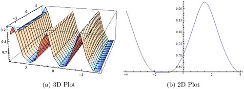
Here, we illustrate our solutions with a few two- and three-dimensional representations. The graphical representation has been provided for the obtained solutions. Figure 1 represents the solitary solution using 3D and 2D graphs. The graphical illustration of the soliton polynomial solution has been depicted in Figure 2. The solutions as rational periodic and soliton types are shown in Figures 3 and 4. There are records of bright solitons, singular solitons and singular periodic solitons.

Figure 1. Graphical representation of Equation (19(19) $u(x,y,z,t)=\ln \left(\frac{{\tanh }^2\left(\frac{(x+y+z)-\mathrm{\beta t}}{2\sqrt{1-{\beta }^2}\sqrt[4]{\frac{1}{n}}}\right)}{\sqrt{\frac{1}{n}}}\right).$(19) ) along z = 0.

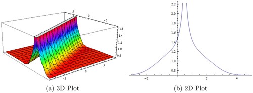
Figure 2. Graphical illustration of Equation (23(23) $u(x,y,z,t)=\ln \left(\frac{\sqrt{q}{(r_1{e}^{\frac{\sqrt[4]{n}((x+y+z)-\mathrm{\beta t})}{\sqrt{1-{\beta }^2}}}+1)}^2}{(r_1{e}^{\frac{\sqrt[4]{n}((x+y+z)-\mathrm{\beta t})}{\sqrt{1-{\beta }^2}}}-1){}^2}\right).$(23) ) along z = 0. (a) 3D Plot3. (b) 2D Plot4.

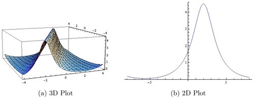
Figure 3. Graphical illustration of Equation (29(29) $\begin{array}{rl}& u(x,y,z,t)\\ & =\ln \left(\frac{\begin{array}{c}\sqrt{n}(\tan \left(\frac{\sqrt{-\sqrt{n}}((x+y+z)-\mathrm{\beta t})}{\sqrt{1-{\beta }^2}}\right)\\ +\sec \left(\frac{\sqrt{-\sqrt{q}}((x+y+z)-\mathrm{\beta t})}{\sqrt{1-{\beta }^2}}\right))\end{array}}{\begin{array}{c}\tan \left(\frac{\sqrt{-\sqrt{q}}((x+y+z)-\mathrm{\beta t})}{\sqrt{1-{\beta }^2}}\right)\\ -\sec \left(\frac{\sqrt{-\sqrt{q}}((x+y+z)-\mathrm{\beta t})}{\sqrt{1-{\beta }^2}}\right)\end{array}}\right).\end{array}$(29) ) along z = 0. (a) 3D Plot5. (b) 2D Plot6.

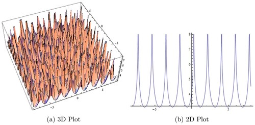
Figure 4. Graphical illustration of Equation (33(33) $\begin{array}{rl}& u(x,y,z,t)\\ & =\ln \left(\frac{\begin{array}{c}(-4\sqrt[4]{n}{c}_1{s_1}^2+4\sqrt{n}{\mathrm{e}}^{\xi \sqrt[4]{n}}{s_1}^2\\ +{\mathrm{e}}^{-\xi \sqrt[4]{n}}{c_1}^2{s_1}^2-4{\mathrm{e}}^{-\xi \sqrt[4]{n}}{c}_1{r}_0{s}_1\\ +4{\mathrm{e}}^{-\xi \sqrt[4]{n}}{r_0}^2+8r_0{s}_1\sqrt[4]{n})\sqrt{n}\end{array}}{\begin{array}{c}4\sqrt{n}{\mathrm{e}}^{\xi \sqrt[4]{n}}{s_1}^2+4\sqrt[4]{n}{c}_1{s_1}^2\\ +{\mathrm{e}}^{-\xi \sqrt[4]{n}}{c_1}^2{c_1}^2-4{\mathrm{e}}^{-\xi \sqrt[4]{n}}{c}_1{r}_0{s}_1\\ +4{\mathrm{e}}^{-\xi \sqrt[4]{n}}{r_0}^2-8r_0{s}_1\sqrt[4]{n}\end{array}}\right),\end{array}$(33) ) along z = 0. (a) 3D Plot7. (b) 2D Plot8.

7. Qualitative analysis of the q-deformed Sinh-Gordon equation

This section includes the bifurcation behaviour for our governing equation. To fulfil this, we transform the model to ordinary differential Equation (7(7) $-2f^{\prime 2}+2f{f}^{″}-f^3+\mathrm{qf}=0.$(7) ), through the travelling wave transformation discussed before.

By using (7(7) $-2f^{\prime 2}+2f{f}^{″}-f^3+\mathrm{qf}=0.$(7) ), the planer dynamic system retrieved is shown below (34) $\begin{array}{rl}& f^{\mathrm{\prime }}=k\\ & k^{\mathrm{\prime }}=\frac{k^2}{2}+\frac{f^2}{2}-\frac{q}{2},\end{array}$(34) but the above system isn't Hamiltonian. From (34(34) $\begin{array}{rl}& f^{\mathrm{\prime }}=k\\ & k^{\mathrm{\prime }}=\frac{k^2}{2}+\frac{f^2}{2}-\frac{q}{2},\end{array}$(34) ), we get (35) $\frac{d{k}^2}{\mathrm{df}}=\frac{f^3-\mathrm{qf}+2k^2}{f},$(35) here f = 0 is singular point of the above equation ; therefore; just in exceptional circumstances could f has a zero. Equation (35(35) $\frac{d{k}^2}{\mathrm{df}}=\frac{f^3-\mathrm{qf}+2k^2}{f},$(35) ) has the following solution (36) $k^2=f^3+\mathrm{qf}+c{f}^2$(36) Then, we get (37) $(f^{\mathrm{\prime }}{)}^2-[f^3-\mathrm{qf}+c{f}^2]=0,$(37) c is the constant of integration. As q and c are constants, it's feasible to obtain equivalent conserved quantity (38) $H(f,k)=k^2-[f^3-\mathrm{qf}+c{f}^2],$(38) that is undoubtedly conserved quantity. Here, we perform a qualitative examination based upon the governing problem implementing the discrimination system. Equation (38(38) $H(f,k)=k^2-[f^3-\mathrm{qf}+c{f}^2],$(38) ) with its potential energy is shown below (39) $F(f)=-[f^3-\mathrm{qf}+c{f}^2],$(39) and thus we get (40) $F^{\mathrm{\prime }}(f)=-3f^2-q-2\mathrm{cf}.$(40) $J(f,k)$ is the coefficient matrix regarding the linearized system at a fixed point $(f,k))$. That is termed as Jocobian. The determinant of that matrix is as follows: (41) $\left|\begin{array}{cc}0& 1\\ -6f-2c& 0\end{array}\right|,$(41) it is convenient to show that the eigenvalues at singular point $(f,0)$ are (42) ${\lambda }_{\pm }(f,0)=\pm \sqrt{-6f-c2},$(42) therefore, $(f,0)$ is saddle if $J(f,0)$ is less than zero, if $J(f,0)$ is greater than zero, then its a centre point whereas it will be cusp if $J(f,0)$ is zero.

Through discriminant of the polynomial (43) $\mathrm{\Delta }=-4c^2-12q,$(43) we get the following outcomes.

Case I:

let $\mathrm{\Delta }=0$ and q>0, then we get (44) $F^{\mathrm{\prime }}(f)=(f-s{)}^2.$(44) In this case, there exist only one equilibrium point (s,0), it will be cusp when n = 3, $c=\pm 3$, we have s = 1 for c = −3, whereas we get s = −1 for c = 3.

Case II:

If $\mathrm{\Delta }>0$, c>0 and q<0, we get (45) $F^{\mathrm{\prime }}(f)=(f-s)(f-t).$(45) we obtain two equilibrium points. For c>0, we have $(s,0)$ that is a saddle but $(t,0)$ will be centre. Phase portrait is shown taking n = −3 and c = −4. We get s = −3 and t = 0.333.

Case III:

If $\mathrm{\Delta }>0$, q<0 and c<0, we get (46) $F^{\mathrm{\prime }}(f)=(f-s)(f-l),$(46) here, two equilibrium points are obtained. For c>0, $(s,0)$ a saddle point and $(l,0)$ is the centre. For n = −3 and c = 4, we get s = −0.333 and l = 3 and the phase portrait is plotted.

Case IV:

If $\mathrm{\Delta }>0$, q = 0 and c>0, we get (47) $F^{\mathrm{\prime }}(f)=f(f-s).$(47) In the above equation, we get two equilibrium points $(0,0)$ with $(s,0)$. Regarding this case $(0,0)$ being a centre, whereas $(s,0)$ is a saddle point. Phase portrait has been plotted for c = 3, where we get s = −2.

Case V:

If $\mathrm{\Delta }>0$, q = 0 and c<0, we get (48) $F^{\mathrm{\prime }}(f)=f(f-p),$(48) We get two equilibrium points $(0,0)$ with $(s,0)$. Here, $(0,0)$ and $(p,0)$ are saddle points. The phase depiction has been plotted for c = −3, where we get s = 2. The phase portrait is shown in Figures 5–8. The red lines represent centre on $(s,0)$ and the lines in cyan colour show the saddle behaviour of $(0,0)$ and the black line shows the saddle behaviour on $(0,0)$ and centre towards $(s,0)$.

Figure 5. Geometric visualization of Equation (38(38) $H(f,k)=k^2-[f^3-\mathrm{qf}+c{f}^2],$(38) ) regarding Case II.

Figure 6. Geometric visualization of Equation (38(38) $H(f,k)=k^2-[f^3-\mathrm{qf}+c{f}^2],$(38) ) regarding Case III.

Figure 7. Geometric visualization of Equation (38(38) $H(f,k)=k^2-[f^3-\mathrm{qf}+c{f}^2],$(38) ) regarding Case IV .

Figure 8. Geometric visualization of Equation (38(38) $H(f,k)=k^2-[f^3-\mathrm{qf}+c{f}^2],$(38) ) regarding Case V .

7.1. Comparitive study

Here, we compare our work with the previous work done on the governing model. The q-deformed Sinh-Gordon problem has been constructed in [36]. Quasi-periodic and chaotic behaviours have been documented with some analytical solutions using different techniques in [39]. The generalized q-deformed Sinh-Gordon equation has been solved numerically using the finite difference method and analytically using the new general form of Kudryashov's strategy in [40]. However, we applied a unified approach which helped to extract different solutions in many ways. Also, we used (3+1) dimensional model which is different from the generalized model, for qualitative analysis. Such work will be useful for further study on such model.

8. Conclusion

This article provided an investigation of the soliton solutions in the (3+1)-dimensional q-deformed Sine-Gordon model and the presence of soliton solutions. For modelling physical systems with violated symmetries, this newly established equation may be helpful. A unified method has been applied to retrieve solutions to the (3+1)-dimensional q-deformed Sinh Gordon model. Polynomial with rational solutions was retrieved in the article. When the appropriate limiting constraints are given to the parameters, this technique successfully retrieves hyperbolic and trigonometric results. Some graphical representations of solutions of the proposed equation are illustrated. Similarly, the impacts of the parameters on the expected non-singular solution are depicted through 2D graphs. Moreover, the qualitative analysis i.e. Bifurcation is performed on the discussed model and sensitive inspection is used to verify the sensitivity of the equation under consideration. The system is converted into a planer Hamiltonian dynamical system using Galilean transformation. The possible cases were predicted and effectively shown in phase portraits based on discriminants. The obtained solutions were novel and they were not shown previously.

Acknowledgement

The authors extend their appreciation to the Deputyship for Research & Innovation, Ministry of Education in Saudi Arabia for funding this research work through the project number RI-44-0077.

Disclosure statement

No potential conflict of interest was reported by the author(s).

Data availability statement

No data were used to support this study.

References

- Yusuf A, Sulaiman TA, Mirzazadeh M, et al. M-truncated optical solitons to a nonlinear Schrodinger equation describing the pulse propagation through a two-mode optical fiber. Opt Quantum Electron. 2021;53(10):558. doi: 10.1007/s11082-021-03221-2
- Haus HA, Wong WS. Solitons in optical communications. Rev Mod Phys. 1996;68(2):423–444. doi: 10.1103/RevModPhys.68.423
- Raza N, Rani B, Chahlaoui Y, et al. A variety of new rogue wave patterns for three coupled nonlinear Maccari's models in complex form. Nonlinear Dyn. 2023;111:18419–18437. doi: 10.1007/s11071-023-08839-3
- Saha Ray S, Sagar B. Numerical soliton solutions of fractional modified (2+1)-dimensional Konopelchenko-Dubrovsky equations in plasma physics. J Comput Nonlinear Dyn. 2022;17(1):011007. doi: 10.1115/1.4052722
- Raza N, Butt AR, Arshed S, et al. A new exploration of some explicit soliton solutions of q-deformed Sinh-Gordon equation utilizing two novel techniques. Opt Quantum Electron. 2023;55(3):200. doi: 10.1007/s11082-022-04461-6
- Ismael HF, Bulut H. Multi soliton solutions, M-lump waves and mixed soliton-lump solutions to the awada-Kotera equation in (2+1)-dimensions. Chin J Phys. 2021;71:54–61. doi: 10.1016/j.cjph.2020.11.016
- Liu C, Dai Z. Exact soliton solutions for the fifth-order Sawada-Kotera equation. Appl Math Comput. 2008;206(1):272–275.
- Rizvi STR, Ali K, Ahmad M. Optical solitons for Biswas-Milovic equation by new extended auxiliary equation method. Optik. 2020;204:164181. doi: 10.1016/j.ijleo.2020.164181
- Serkin VN, Hasegawa A. Novel soliton solutions of the nonlinear Schrödinger equation model. Phys Rev Lett. 2000;85(21):4502–4505. doi: 10.1103/PhysRevLett.85.4502
- Hirota R, Satsuma J. Soliton solutions of a coupled Korteweg-de Vries equation. Phys Lett A. 1981;85(8-9):407–408. doi: 10.1016/0375-9601(81)90423-0
- Hirota R. Soliton solutions to the BKP equations. I. The Pfaffian technique. J Phys Soc Japan. 1989;58(7):2285–2296. doi: 10.1143/JPSJ.58.2285
- Kaplan M, Bekir A, Akbulut A. A generalized Kudryashov method to some nonlinear evolution equations in mathematical physics. Nonlinear Dyn. 2016;85:2843–2850. doi: 10.1007/s11071-016-2867-1
- Arshed S, Raza N, Butt AR, et al. Multiple rational rogue waves for higher dimensional nonlinear evolution equations via symbolic computation approach. J Ocean Eng Sci. 2023;8:33–41. doi: 10.1016/j.joes.2021.11.001
- Akbar MA, Ali NHM, Islam MT. Multiple closed form solutions to some fractional order nonlinear evolution equations in physics and plasma physics. AIMS Math. 2019;4(3):397–411. doi: 10.3934/math.2019.3.397
- Kumar S. Numerical computation of time-fractional Fokker-Plank equation arising in solid state physics and circuit theory. Z Naturforsch A. 2013;68a:777–784.
- Bekir A. Application of the (G' G)-expansion method for nonlinear evolution equations. Phys Lett A. 2008;372(19):3400–3406. doi: 10.1016/j.physleta.2008.01.057
- Geng X, Ma Y. N-soliton solution and its Wronskian form of a (3+1)-dimensional nonlinear evolution equation. Phys Lett A. 2007;369(4):285–289. doi: 10.1016/j.physleta.2007.04.099
- Lou SY. Extended Painlevé expansion, nonstandard truncation and special reductions of nonlinear evolution equations. Z Naturforsch A. 1998;53(5):251–258. doi: 10.1515/zna-1998-0523
- Satsuma J. Hirota bilinear method for nonlinear evolution equations. In: Direct and inverse methods in nonlinear evolution equations: lectures given at the CIME summer school held in Cetraro, Italy; 1999 Sep 5–12; Berlin, Heidelberg: Springer; 2003. p. 171–222.
- Ismael HF, Sulaiman TA, Osman MS. Multi-solutions with specific geometrical wave structures to a nonlinear evolution equation in the presence of the linear superposition principle. Commun Theor Phys. 2022;75(1):015001. doi: 10.1088/1572-9494/aca0e2
- Kawata T, Inoue H. Inverse scattering method for the nonlinear evolution equations under nonvanishing conditions. J Phys Soc Japan. 1978;44(5):1722–1729. doi: 10.1143/JPSJ.44.1722
- Svirshchevskii SR. Invariant linear spaces and exact solutions of nonlinear evolution equations. J Nonlinear Math Phys. 1996;3(1-2):164–169. doi: 10.2991/jnmp.1996.3.1-2.20
- Kumar S, Kumar D, Kharbanda H. Lie symmetry analysis, abundant exact solutions and dynamics of multisolitons to the (2+1)-dimensional KP-BBM equation. Pramana. 2021;95(1):33. doi: 10.1007/s12043-020-02057-x
- Kumar S, Kumar D. Lie symmetry analysis and dynamical structures of soliton solutions for the (2+1)-dimensional modified CBS equation. Int J Mod Phys B. 2020;34(25):2050221. doi: 10.1142/S0217979220502215
- Kumar S, Rani S. Lie symmetry reductions and dynamics of soliton solutions of (2+1)-dimensional Pavlov equation. Pramana. 2020;94(1):116. doi: 10.1007/s12043-020-01987-w
- Kumar S, Almusawa H, Kumar A. Some more closed-form invariant solutions and dynamical behavior of multiple solitons for the (2+1)-dimensional rdDym equation using the Lie symmetry approach. Results Phys. 2021;24:104201. doi: 10.1016/j.rinp.2021.104201
- Kumar S, Kumar D, Wazwaz AM. Lie symmetries, optimal system, group-invariant solutions and dynamical behaviors of solitary wave solutions for a (3+1)-dimensional KdV-type equation. Eur Phys J Plus. 2021;136(5):531. doi: 10.1140/epjp/s13360-021-01528-3
- Kumar D, Kumar S. Some new periodic solitary wave solutions of (3+1)-dimensional generalized shallow water wave equation by Lie symmetry approach. Comput Math Appl. 2019;78(3):857–877. doi: 10.1016/j.camwa.2019.03.007
- Zhong WP, Belic MR, Petrovic MS. Solitary and extended waves in the generalized Sinh-Gordon equation with a variable coefficient. Nonlinear Dyn. 2014;76:717–723. doi: 10.1007/s11071-013-1162-7
- Yang Z, Zhong WP. Analytical solutions to Sine-Gordon equation with variable coefficient. Rom Rep Phys. 2014;66(2):262–273.
- Zhong WP, Belic M. Special two-soliton solution of the generalized Sine-Gordon equation with a variable coefficient. Appl Math Lett. 2014;38:122–128. doi: 10.1016/j.aml.2014.07.015
- Raza N, Rafiq MH, Kaplan M, et al. The unified method for abundant soliton solutions of local time fractional nonlinear evolution equations. Results Phys. 2021;22:103979. doi: 10.1016/j.rinp.2021.103979
- Raza N, Jhangeer A, Arshed S, et al. Dynamical analysis and phase portraits of two-mode waves in different media. Results Phys. 2020;19:103650. doi: 10.1016/j.rinp.2020.103650
- Saha A. Bifurcation, periodic and chaotic motions of the modified equal width-Burgers (MEW-Burgers) equation with external periodic perturbation. Nonlinear Dyn. 2017;87(4):2193–2201. doi: 10.1007/s11071-016-3183-5
- Alharbi AR, Almatrafi MB. Exact solitary wave and numerical solutions for geophysical KdV equation. J King Saud Univ Sci. 2022;34(6):102087. doi: 10.1016/j.jksus.2022.102087
- Eleuch H. Some analytical solitary wave solutions for the generalized q-deformed Sinh-Gordon equation. Adv Math Phys. 2018;2018:5242757.
- Ali KK, Abdel-Aty AH. An extensive analytical and numerical study of the generalized q-deformed Sinh-Gordon equation. J Ocean Eng Sci. 2022. doi: 10.1016/j.joes.2022.05.034
- Alrebdi HI, Raza N, Arshed S, et al. A variety of new explicit analytical soliton solutions of q-deformed Sinh-Gordon in (2+1) dimensions. Symmetry. 2022;14(11):2425. doi: 10.3390/sym14112425
- Kazmi SS, Jhangeer A, Raza N, et al. The analysis of bifurcation, quasi-periodic and solitons patterns to the new form of the generalized q-deformed Sinh-Gordon equation. Symmetry. 2023;15(7):1324. doi: 10.3390/sym15071324
- Ali KK. Analytical and numerical study for the generalized q-deformed Sinh-Gordon equation. Nonlinear Eng. 2023;12(1):20220255. doi: 10.1515/nleng-2022-0255