
 ?Mathematical formulae have been encoded as MathML and are displayed in this HTML version using MathJax in order to improve their display. Uncheck the box to turn MathJax off. This feature requires Javascript. Click on a formula to zoom.
Abstract
Our article proves inequalities for interval optimization and shows that feasible and descent directions do not intersect in constrained cases. Mainly, we establish some new interval inequalities for interval-valued functions by defining LC-partial order. We use LC-partial order to study Karush–Kuhn–Tucker (KKT) conditions and expands Gordan's theorems for interval linear inequality systems. By applying Gordan's theorem, we can determine the best outcomes for interval optimization problems (IOPs) that have constraints, such as Fritz John and KKT conditions. The optimality conditions are observed with inclusion relations rather than equality. We can use the KKT condition for binary classification with interval data and support vector machines(SVMs). We present some examples to illustrate our results.
1. Introduction
Optimization theory is applied in a variety of industries, including engineering. Data collection and quantification are crucial in modelling an optimization problem. An optimization model's data is typically derived through measurements or observations. Frequently, acquired data sets are published with an error percentage or imprecision. Fuzzy numbers or intervals are appropriate representations for such data. As a result, the various parameters/coefficients used for the formulation of the modelled constraint and objective functions using obtained data, are converted to intervals or fuzzy numbers.
Optimization is the process of determining the best available values across a collection of inputs to maximize or minimize an objective function. Whether utilizing supervised or unsupervised learning, all deep learning models require some variance in optimization.
IOPs have been the subject of various investigations. Based on the worst- or best-case situations, many current strategies optimize the objective function's upper or lower function or their mean. Consequently, conventional methods of optimization can address the resulting problem of IOP, transforming it into single-valued optimization problems based on worst- or best-case situations and numerous current strategies that optimize the objective function's upper or lower function or their mean. IOPs have also been subjected to the KKT optimality conditions. Wu, did a lot of research on it [Citation1–3].
Using a generalized derivative, Chalco-Cano [Citation4] proposed KKT optimality conditions for IOPs. The generalized derivatives and the partial ordering of intervals were utilized by Singh et al. [Citation5,Citation6] to define KKT conditions for the IOPs combining upper and lower functions. It is important to note that current research on IOP optimality conditions used algebraic manipulations rather than a geometrical analysis of an optimal point in order to generalize existing optimality conditions.
Mathematical and theoretical modelling are crucial components of optimization problems [Citation7]. Practically, determining the coefficients of an objective function as a real number is generally difficult. Since a wide range of real-world problems can involve data imprecision due to measurement errors or other unanticipated circumstances. Robust optimization [Citation8] and interval-valued optimization are two methods of deterministic optimization that deal with unknown data.
Slowinski and Teghem compared two different optimization problems for multi-objective programming problems [Citation9]. The KKT optimality criteria have been studied for over a century and play a significant role in optimization theory. Wu [Citation1], Dar, and Singh [Citation6] developed KKT optimality conditions for optimization problems with interval-valued objective functions and constraints. Lodwick and Chalco-Cano [Citation4] used the generalized derivative to examine the interval-valued optimization problem's KKT optimality criteria.
SVMs are a type of machine learning technique that may be used to classify and predict data. Training and testing data are required for the development of a SVM [Citation10]. The user sorts the training data into the appropriate categories. An optimization problem is used to create a model using this data. This model generates a hyperplane that divides the testing data set into the right categories in a linear manner.
SVMs are cutting-edge machine-learning approaches with a foundation in structural risk minimization [Citation11,Citation12]. The structural risk minimization theory states that a function from a function class has a low expectation of risk on all data from an underlying distribution if that a function has a low empirical risk on a particular data set sampled from that distribution and the function class has a low level of complexity, as determined by Vapnik [Citation13]. By utilizing the fact that a bigger margin correlates with a smaller fat-shattering dimension for the particular function classes, the well-known large margin technique in SVMs [Citation14] fundamentally limitize the complexity of the function class.
The derivative is the most commonly used term in classical optimization theory. In constrained optimization problems, it is useful for studying optimality criteria and duality theorems. H-derivative is a well-known notion. But the H-derivative has limitations. Luciano and Stefanini [Citation15] proposed the gH-derivative in 2009 to address the shortcomings of the H-derivative. These IVF versions have been widely used by optimal problem researchers. For example, Wu [Citation3] used H-derivative to examine the KKT conditions for nonlinear IOPs.
It is impossible to overestimate the importance of derivatives in IOP problems that are nonlinear. Wu [Citation1–3] explored interval-valued nonlinear programming problems and showed how the H-derivative may be used in interval-valued KKT optimization problems. The gH-differentiability was also extended to learn interval-valued KKT optimality conditions, according to Chalco-Cano [Citation4].
Ghosh et al. used extended KKT conditions for IOPs in their study [Citation16] to apply them to interval-valued SVMs using LU-partial order. In [Citation17,Citation18], researchers recently discussed a generalized interval-valued portfolio optimization problem. It is well known that a set of all compact intervals is a partially ordered set. In [Citation19], Younus et al. defined several partial orders of
and obtained relationships between them. They have shown that LC-partial order is not equivalent to LU-partial order. However, LC-partial order implies LU-partial order. For some interesting results, see, also, Dastgeer et al. [Citation20]. Building on the previous studies, we extended the results of [Citation16] for LC-partial order and identified some variations. Motivated by gH-differentiability of interval-valued functions and latest LC -partial order, we discuss all optimality conditions and SVM problem under gH-differentiability and LC-partial order. Which generalized many results in the literature.
We would now like to outline the contributions of this work.
Interval optimization inequalities: The article introduces and proves inequalities specifically tailored for IOPs. This suggests a departure from traditional optimization techniques and an exploration of methods suited to handling intervals.
Non-intersecting directions: In constrained scenarios, the article demonstrates that feasible and descent directions do not intersect. This observation likely has implications for optimization algorithms and could lead to more efficient optimization strategies.
LC-partial order: The authors introduce the concept of LC-partial order, a new mathematical framework that appears to be a key component of their approach. This concept may have applications beyond the specific problem discussed in the article.
Extension of Gordan's theorems: The article extends Gordan's theorems to interval linear inequality systems. This extension could have broader implications in mathematical theory and its application to optimization.
Inclusion-based optimality conditions: Instead of traditional equality-based optimality conditions, the article suggests the use of inclusion relations for constrained IOPs. This shift in perspective may lead to new insights and methods for solving such problems.
Application to binary classification: The article highlights the application of KKT conditions for binary classification with interval data and support vector machines. This application demonstrates the practical relevance of the theoretical developments presented in the article.
Illustrative examples: The authors provide examples to illustrate their results, which can help readers to understand the practical implications and potential applications of their findings.
Section 2 provides the basic concepts, definitions, and notations used in the article. The KKT and Fritz John's criteria for IOPs are derived in Section 3 along with extended Gordan's theorems. For both constrained and unconstrained IOPs, we develop the optimality conditions. In Section 4, we apply the optimality conditions given in Section 3 to solve the SVM classification problem on the interval-valued data set. We provide an example of the generated classifier. We give a graphical representation of the classification problem. We also present the conclusion and future scope in Section 5.
2. Preliminaries
Notations
We used the following notations throughout this article:
All the capital and bold letters denote the interval-valued functions or intervals.
represents the set of all bounded and closed intervals in
Sets are represented by ordinary capital letters.
Definition 2.1
The addition and subtraction of intervals and
are defined by
Similarly, for scalar multiplication
where k is the real constant. It can be seen that the definition of interval-difference has the following two limitations
(i) , and
(ii) for , the relation
does not necessarily hold.
Definition 2.2
[21]
Let and
be two intervals in
. The gH-difference between two intervals is defined by
Definition 2.3
Let and
be an interior point of A such that
and there exist
such that
. Let
be a function such that we define
if
exists. Then
is said to have the jth gH-partial derivative at
and It is represented by
,
. The gH-partial derivatives of
at
can be written as
Definition 2.4
Consider an interval-valued function . The gH-gradient of
at any point
is a vector defined by
Definition 2.5
Consider a function .
is called gH-differentiable at
if there exist two functions (interval-valued)
and
such that
for
for some
, where
and
is a function such that
Definition 2.6
[Citation19]
For two intervals and
, we define LC-partial order as:
, if
where
Definition 2.7
A vector y which gives the minimum value of the objective function in an optimization problem over the set of vectors satisfying the constraints
, is called an optimal solution.
Lemma 2.8
For any and
in
such that
, then
.
Proof.
Let and
be two intervals in
such that
Suppose that
, then
It implies that
(1)
(1) and
(2)
(2) As we know that
Case 1: If
, then
and from inequality (Equation1
(1)
(1) ), we have
It implies that
(3)
(3) From (Equation2
(2)
(2) )
it follows
(4)
(4) From (Equation3
(3)
(3) ) and (Equation4
(4)
(4) )
Case 2: If , then
From (Equation1
(1)
(1) )
(5)
(5) from (Equation5
(5)
(5) ) and (Equation4
(4)
(4) )
This completes the proof.
Remark 2.9
Let and
such that
We know from [22]:
If
, then
and if
,
3. KKT conditions under LC-partial order
Definition 3.1
Let A be a convex subset of . We say that an interval-valued function
is LC-convex on A, if for any
and
in A
Theorem 3.2
Let be gH-differentiable at
. Then
exists for every k in
and
Proof.
See [23].
Theorem 3.3
Let A be a non-empty open convex subset of and
be gH-differentiable at any
. Then
is LC-convex on A if and only if
Proof.
Let be LC-convex on A, and any
. Then, for
and
,
By Lemma 2.8, we have
Hence, the above inequality can be written as
(6)
(6) As
, then by Definition 2.5 and Theorem 3.2
where
and
Therefore
Let
in the inequality (Equation6
(6)
(6) ), we get
which is the desired result.
Now for the converse part, let
be true for any
and
in A.
Then, for any , we denote
Hence, the following inequalities hold true
(7)
(7) and
(8)
(8) Multiplying inequality (Equation7
(7)
(7) ) by β and inequality (Equation8
(8)
(8) ) by
, we get
(9)
(9) and
(10)
(10) By adding inequalities (Equation9
(9)
(9) ) and (Equation10
(10)
(10) ), we obtain
By rearranging the above inequality, we obtain
Substituting the value of
in the above inequality, we have
The arbitrariness of
proves that
is LC-convex on A.
Theorem 3.4
Consider an interval-valued function , which is gH-differentiable at
. If a vector
which satisfies
, then there exists
such that for each
,
Proof.
As is gH-differentiable at
, from Definition 2.5 and Theorem 3.2, we have
where
as
. By replacing
, for
, we get
Since,
and
as
, we have
for each
, for some
.
Definition 3.5
Let be an interval-valued function. If
is gH-differentiable at
, the set of descent directions at
is given by the set
For any v in
,
for all
, the set
is said to be the cone of descent directions.
Definition 3.6
For a non-empty set and
, the cone of feasible directions of A at
is given by
Definition 3.7
A feasible solution is said to be an efficient solution of the IOP
(11)
(11) if there does not exist any
in
such that
, where
is a δ-neighbourhood of
. If a solution
is an efficient solution, then we say that
is a non-dominated solution to the IOP.
Theorem 3.8
For a non-empty set , let us consider the following IOP
where
. If
is gH-differentiable at
and
is a local efficient solution to the IOP (Equation11
(11)
(11) ), then
.
Proof.
Contrarily, suppose that and v be an element in
. Then, by Theorem 3.4 there exists
such that
By Definition 3.6, there exists
such that
Let us define
, we note that
,
It is a contradiction to
a local efficient solution. Hence,
Next example illustrates the necessary condition given in Theorem 3.8
Example 3.9
Let be the set
. Let the IOP
(12)
(12) where
. Furthermore,
The lower and upper functions are shown in the above figure. It is verified that is an efficient point. The cone of feasible directions at
is given by
The gH-partial derivatives of
at
are
The cone of descent directions at
is given as
which is not possible. Hence,
Therefore,
Lemma 3.10
Let us consider the set for the interval-valued functions
, where
is an open set in
. Let
and
. Suppose
to be gH-differentiable at
and gH-continuous for
, we define
Then,
where
Proof.
Consider v to be an element in . As
and A is an open set, there exists
such that
For each
, as
is gH-continuous at
where
as
. Since
for
, there exists
such that
As we know that
, for each
there exists
such that by Theorem 3.4
Suppose
. It is evident that
. From the above inequalities, we note that the points of the form
belong to R for each
. Therefore,
. Hence,
Theorem 3.11
Let be an open set in
. Let us consider an IOP
such that
where
and
for
. For a feasible point
, define
. Consider at
,
and
,
, be gH-differentiable, and for
,
be gH-continuous. If
is an efficient solution of the IOP, then
where
and
Proof.
By using Theorem 3.8 and Lemma 3.10, we can conclude that, is a local efficient solution
Theorem 3.12
For an interval-valued vector in
, only one of these given systems has a solution:
Proof.
Consider is true. Let us prove that
must be false. Contrarily, let
be also true. Since
is true, we have
consequently,
it can also be written as
(13)
(13) As
is also true, then
also, we have
(14)
(14) As (Equation13
(13)
(13) ) and (Equation14
(14)
(14) ) cannot be true together, so we have contradiction here. Hence, if
is true,
cannot be true. For the other case, Let us suppose that
is false. We prove that
is true. Contrarily, Let us suppose
is false. Therefore,
Consequently,
(15)
(15) Let the sets
and
By (Equation15
(15)
(15) ) it can be seen that
. Also
and
. Let us create a vector
such that
For this
, we can see that
More generally,
(16)
(16) As
is false, then
Which is a contradiction to (Equation16
(16)
(16) ). So (ii) must be true. Which completes the proof.
Theorem 3.13
If is a local efficient solution to the following IOP
then
, where
is gH-differentiable at
,
Proof.
By using Definition 3.4 and Theorem 3.5, if is a local efficient solution, then
. Consequently,
From Theorem 3.12 with
,
,
, such that
Remark 3.14
It is very interesting to observe that the optimality condition in the above theorem is not an equality relation but an inclusion relation
. Inclusion relations are less restrictive and more correct than equality relations. For example if
then
but
.
Theorem 3.15
For an interval-valued matrix , where
, only one of the given systems has a solution:
Proof.
Consider is true. Let us prove that
is false. Contrarily, consider
is also true. Since, (i) is true, we have
Consequently,
Then, it can be written as
(17)
(17) As we considered
is also true, then for some non-zero
, where
. Now we have
(18)
(18) Consider
. It implies that
and
From (Equation18
(18)
(18) ), we have
Then, it can be written as
(19)
(19) As (Equation17
(17)
(17) ) and (Equation19
(19)
(19) ) cannot be true together, so here is a contradiction. Hence, (ii) cannot be true if
is true.
For this, Let us suppose that is not true. We shall prove that
is true. If
is not true, then
(20)
(20) Let us suppose, contrarily, that
is also false. Then,
Consequently,
it implies that
(21)
(21) where
. Let the sets
and
By (Equation21
(21)
(21) ), it can be seen that
. Also
and
. Let us create a vector
by
For this
, we notice that
which is equivalent to
(22)
(22) The inequality (Equation22
(22)
(22) ) can be true only when
. The inequalities (Equation20
(20)
(20) ) and (Equation22
(22)
(22) ) are contradictory, so
and
cannot hold together. Hence,
must be true. This completes the proof.
Theorem 3.16
Let be a set in
;
and
for
. Consider IOP
(23)
(23) Let
be a feasible point of IOP (Equation23
(23)
(23) ), we define
Suppose,
and
are gH-differentiable at
for
and gH-continuous for
. If
is a local efficient point of (Equation23
(23)
(23) ), then there exist constants
and
for
such that
where,
is the vector whose components are
for
. Furthermore, if
are also gH-differentiable at
, then there exist
constants such that
where, w is the vector
.
Proof.
As is a local efficient point of (Equation23
(23)
(23) ), by Theorem 3.11, we get
or we can say that
such that
(24)
(24) Let
be the matrix such that
By (Equation24
(24)
(24) ) we notice that
Now by Theorem 3.15,
,
such that
Consider q of the form
(25)
(25) by putting (Equation25
(25)
(25) ) in
, we have
by simplifying the above expression, we have
The first part of the theorem is proved here.
For the second part, suppose for ,
. Consequently,
If
,
are also gH-differentiable at
, then by setting
for
we have
which completes our proof.
Definition 3.17
The collection of n interval vectors is called linearly independent if for n real numbers
otherwise dependent.
Example 3.18
Let and
.
Now we have
and
So, it is a linearly independent set of interval vectors.
Theorem 3.19
Let be a subset of
and
and
for
be IVFs. Let
be a feasible point of the following IOP
We define
Suppose,
and
are gH-differentiable at
for
and gH-continuous for
. Consider the interval vectors
are linearly independent and if
is an efficient solution then there exist scalars
such that
Furthermore, if
for
are also gH-differentiable at
, then there exist
constants such that
Proof.
By Theorem 3.16, and
, where
and
are real constants and not all zeros, such that
We need to have
. Because in another case, the set
will become linearly dependent. We define
then,
for all
and
For
,
. Thus,
. If the functions
for
are also gH-differentiable at
, then by setting
for
we have
which proves the second part of our theorem.
To illustrate the necessary conditions given in Theorems 3.16 and 3.19, let consider a detail example.
Example 3.20
Consider the IOP with feasible point
such that
In this IOP, the functions
,
, and
are gH-differentiable on
. We notice that, at
Now, we find gH-partial derivatives of
by using Definition 2.3,
Thus,
. We notice that
We don't actually need
because
. Therefore only
is enough. Now, the conclusions in Theorem 3.16 hold for
,
and
as
And that of Theorem 3.19 hold for
,
and
as
Theorem 3.21
Let be an open convex set such that
and
,
be gH-differentiable LC-convex functions on A. Let
be a feasible point of the IOP
If there exist
scalars such that
Then
is an efficient solution of the IOP.
Proof.
By supposition, for every satisfying
. We have
By using Theorem 3.3
Therefore, for every
,
In either case,
is an efficient solution to the considered IOP. Here is the proof.
4. Applications of KKT conditions in SVM
Let us consider a binary classification problem. For a data set
the problem of classifying data using SVMs is identical to the optimization problem below:
(26)
(26) where
is the weight vector and
is the bias.
The constraints specify that the data points must be on opposite sides of the separating hyperplanes . There is uncertainty and imprecision in the data set in many classification problems. This might be due to errors in measurement, implementation, and so on.
For example, weather problems include interval-type data because we cannot find the weather condition for an instant of time, it is always for some duration and other circumstances during that time duration. And the inequality (Equation26(26)
(26) ) does not deal with interval-type data. As a result, the SVM problem is adjusted for the interval-valued data set
by
By adjusting the above problem accordingly, we get
(27)
(27) We can see that
and
are both gH-differentiable and LC-convex functions. These functions of gH-gradients are as follows:
where
and
are the gH-partial derivatives corresponding to z and d, respectively.
By Theorem 3.19, for an efficient point of (Equation27
(27)
(27) ) there exist non-negative constants
such that
(28)
(28) and
(29)
(29) The condition (Equation28
(28)
(28) ) can be written as
and
The points in the data
for which
are called support vectors. From (Equation29
(29)
(29) ), we notice that corresponding to any
, we have
. Therefore, with respect to
, the value of the bias
is such a value that
for which
.
Since, the functions and
are gH -differentiable and LC-convex, by using Theorems 3.19 and 3.21, the collection of conditions that we must solve in order to find efficient solutions of the SVM IOP (Equation27
(27)
(27) ) are
(30)
(30) For any of the values of z that fulfill the condition in (Equation30
(30)
(30) ), let us define the set of possible values of the bias as
(31)
(31) By using any solution
and
of (Equation30
(30)
(30) ) and (Equation31
(31)
(31) ), a classifying hyperplane and the SVM classifier function are given respectively
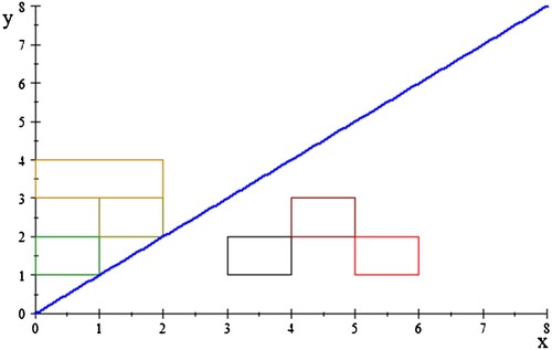
Example 4.1
Let us consider the interval data set
Let us find a classifying hyperplane for the above data set.
For finding a classifying hyperplane, the possible solution to (Equation30
(30)
(30) ) with respective
are required.
For the choice , we notice that we have
According to the first condition (Equation30
(30)
(30) ), the values of
for which
are
and
. The condition in (Equation30
(30)
(30) ) becomes
(32)
(32) where
Substituting in (Equation32
(32)
(32) ), we have
As
, and we are working on
so, n = 2. As a result
, which means
. The above condition becomes
We choose
and
. Corresponding to this
, from (Equation31
(31)
(31) ) and the condition 3 in (Equation30
(30)
(30) ), the set of possible values for the bias d is as follows
Since,
,
. Then, for i = 1, we have
upon simplification and setting
we get
By applying the definition of gH-difference there are 2 cases by the first Lemma, that is
or
. But it does not matter because of equality with
For
, we have
(33)
(33) Similarly, for i = 6
upon simplification, we get
For
, we have
This implies that
(34)
(34) Now, we have
Substituting (Equation33
(33)
(33) ) and (Equation34
(34)
(34) ) in the above expression
Therefore, corresponding to
and
, the expression for the classifying hyperplane (see Figure ) is as follows
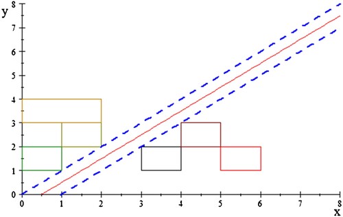
Similarly, we can find equations for other hyperplanes.
Figure 1. The objective function of example.
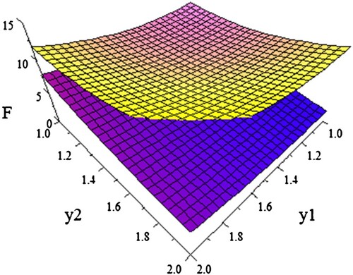
Figure 2. The hyperplane represents .
Now, we give a graphical representation of the hyperplane by the following figure.
By translating the above equation, we can get more equations for classifying hyperplane by the following Figure . The blocks in Figure show the interval data set considered in the example. The red hyperplane is the best classifying hyperplane which represents the equation and the blue dotted lines are margin lines that represent the equations
and
. And the strip, which is formed by the equations
and
, contains all the hyperplanes that classify the given data.
Figure 3. An interval-valued classifying hyperplane.
5. Conclusion
In this article, we considered the constrained IOP for characterizing the efficient solution. We generalized Gordan's theorems to get the Fritz–John condition for IOPs. We also derived an extension to KKT's necessary optimality condition for LC-partial order. The derived conditions formed the basis of our expression for SVMs, and we demonstrated how SVMs classify data using KKT conditions. To get hyperplane in interval-valued vectors is not a simple task. In Example 4.1, we only consider a very small data set. For a large data set, it can be more complex. Also in this article, we only tackle a non-overlapping data set. For overlapping data set, it will not work. Therefore, in the future, SVM regression analysis might apply to the SVM classifier and also one can discuss overlapping data set and also generalized this idea for multi-classification problem.
Authors' contributions
All authors contributed equally to this article. They have read and approved the final manuscript.
Disclosure statement
The authors confirm that there are no known conflicts of interest associated with this publication.
References
- Wu HC. The Karush–Kuhn–Tucker optimality conditions in multiobjective programming problems with interval-valued objective functions. Eur J Oper Res. 2009;196:49–60. doi: 10.1016/j.ejor.2008.03.012
- Wu HC. On interval-valued nonlinear programming problems. J Math Anal Appl. 2008;338:299–316. doi: 10.1016/j.jmaa.2007.05.023
- Wu HC. The Karush–Kuhn–Tucker optimality conditions in an optimization problem with interval-valued objective function. Eur J Oper Res. 2007;176:46–59. doi: 10.1016/j.ejor.2005.09.007
- Chalco-Cano Y, Lodwick WA, Rufian-Lizana A. Optimality conditions of type KKT for optimization problem with interval-valued objective function via generalized derivative. Fuzzy Optim Decis Mak. 2013;12:305–322. doi: 10.1007/s10700-013-9156-y
- Singh D, Dar B, Kim DS. KKT optimality conditions in interval valued multiobjective programming with generalized differentiable functions. Eur J Oper Res. 2016;254:29–39. doi: 10.1016/j.ejor.2016.03.042
- Singh D, Dar BA, Goyal A. KKT optimality conditions for interval valued optimization problems. J Nonlinear Anal Optim. 2014;5:91–103.
- Slyn'ko VI, Tunç C. Instability of set differential equations. J Math Anal Appl. 2018;467:935–947. doi: 10.1016/j.jmaa.2018.07.048
- Ben-Tal A, El Ghaoui L, Nemirovski A. Robust optimization. Princeton (NJ): Princeton University Press; 2009. (Princeton Series in Applied Mathematics).
- Slowinski R, Teghem J. Stochastic versus fuzzy approaches to multiobjective mathematical programming under uncertainty. Edited by Roman Słowiński and Jacques Teghem. Theory and Decision Library. Series D: System Theory, Knowledge Engineering and Problem Solving, 6. Kluwer Academic Publishers Group, Dordrecht, 1990.
- Snyder CThe optimization behind support vector machines and an application in handwriting recognition; 2016; p. 1–15.
- Shawe-Taylor J, Bartlett PL, Williamson RC, Anthony M. Structural risk minimization over data-dependent hierarchies. IEEE Trans Inform Theory. 1998;44:1926–1940. doi: 10.1109/18.705570
- Vapnik V. Estimation of dependences based on empirical data. Translated from the Russian by Samuel Kotz. Springer Series in Statistics. Springer-Verlag, New York–Berlin, 1982.
- Vapnik VN. The nature of statistical learning theory. New York: Springer-Verlag; 1995.
- Boser BE, Guyon IM, Vapnik VN. A training algorithm for optimal margin classifiers. Proceedings of the fifth annual workshop on Computational learning theory. 1992; p. 144–152.
- Stefanini S, Bede B. Generalized Hukuhara differentiability of interval-valued functions and interval differential equations. Nonlinear Anal. 2009;71:1311–1328. doi: 10.1016/j.na.2008.12.005
- Ghosh D, Singh A, Shukla KK, et al. Extended Karush–Kuhn–Tucker condition for constrained interval optimization problems and its application in support vector machines. Inform Sci. 2019;504:276–292. doi: 10.1016/j.ins.2019.07.017
- Debnath AK, Ghosh D. Generalized-Hukuhara penalty method for optimization problem with interval-valued functions and its application in interval-valued portfolio optimization problems. Oper Res Lett. 2022;50:602–609. doi: 10.1016/j.orl.2022.08.010
- Kumar K, Ghosh D, Kumar G. Weak sharp minima for interval-valued functions and its primal-dual characterizations using generalized Hukuhara subdifferentiability. Soft Comput. 2022;26:10253–10273. doi: 10.1007/s00500-022-07332-0
- Younus A, Nisar O. Convex optimization of interval valued functions on mixed domains. Filomat. 2019;33:1715–1725. doi: 10.2298/FIL1906715Y
- Dastgeer Z, Younus A, Tunç, C. Distinguishability of the descriptor systems with regular pencil. Linear Algebra Appl. 2022;652:82–96. doi:10.1016/j.laa.2022.07.004
- Chalco-Cano Y, Rufián-Lizana A, Román-Flores H, et al. Calculus for interval-valued functions using generalized Hukuhara derivative and applications. Fuzzy Sets Syst. 2013;219:49–67. doi: 10.1016/j.fss.2012.12.004
- Tao J, Zhang ZH. Properties of interval vector-valued arithmetic based on gH-difference. Math Comput. 2015;4:7–12.
- Ghosh D. Newton method to obtain efficient solutions of the optimization problems with interval-valued objective functions. J Appl Math Comput. 2017;53:709–731. doi: 10.1007/s12190-016-0990-2