Quantifying local predictability of the Lorenz system using the nonlinear local Lyapunov exponent

Abstract

The nonlinear local Lyapunov exponent (NLLE) can be used as a quantification of the local predictability limit of chaotic systems. In this study, the phase-spatial structure of the local predictability limit over the Lorenz-63 system is investigated. It is found that the inner and outer rims of each regime of the attractor have a high probability of a longer than average local predictability limit, while the center part is the opposite. However, the distribution of the local predictability limit is nonuniformly organized, with adjacent points sometimes showing quite distinct error growth. The source of local predictability is linked to the local dynamics, which is related to the region in the phase space and the duration on the current regime.

摘要

非线性局部Lyapunov指数(NLLE)可以用来度量混沌系统的局地可预报性。本文基于NLLE方法研究了Lorenz吸引子在相空间上的局地可预报性的空间分布特征。结果表明，在吸引子两翼的内、外边缘的局地可预报性期限较高，而吸引子中部地区的局地可预报性期限则较低。然而，局地可预报性期限的分布却没有呈现有组织的均一结构，相邻两点的局地可预报性期限可能差别很大。局地可预报性的来源被认为与吸引子上的局地动力学有关，由所在位置和在当前状态的持续时间决定。

Keywords:

• Nonlinear local Lyapunov exponent
• local predictability limit
• chaotic system
• Lorenz system

关键词:

• 非线性局部Lyapunov指数
• 局地可预报性期限
• 混沌系统
• Lorenz吸引子

1. Introduction

The atmosphere is a chaotic system that is sensitive to initial conditions (Li and Chou 1997). The problem of atmospheric predictability has been researched for several decades, since the pioneering work of Thompson and Lorenz (Lorenz 1963, 1965, 1969a, 1969b; Thompson 1957). The main achievement of these early studies was the exploration of the intrinsic limit of predictability in weather forecasting (Chou 1989; Feng et al. 2001; Mu, Duan, and Wang 2002).

As one of several dynamical methods, the global Lyapunov exponent can be used as a measure of the mean divergence rate of nearby trajectories on a strange attractor (Eckmann and Ruelle 1985; Sano and Sawada 1985; Wolf et al. 1985). Given a dynamical system with an initial perturbation of size δ, if the accepted error tolerance is still sufficiently small, then the largest Lyapunov exponent gives a rough estimate of the predictability limit: . Prediction becomes meaningless beyond the predictability limit owing to the propagation of initial errors over the entire chaotic attractor (Wang et al. 2012).

However, we are often more interested in the quantification of the local predictability limit (Ding, Li, and Ha 2008; He et al. 2006). The identification of regions of high and low predictability is of critical importance to numerical weather forecasts. Nese (1989) investigated both the temporal and phase-spatial variations of short-term predictability using local divergence rates for the Lorenz attractor. He concluded that predictability varies considerably with time, while at the same time phase-spatial organization to the variability exists. Mukougawa, Kimoto, and Yoden (1991) adopted the Lorenz index, which gives the amplification rate of the root-mean-square error during a prescribed time interval to measure the local predictability, and obtained the organization on the Lorenz attractor. Abarbanel, Brown, and Kennel (1991) defined the so-called finite time Lyapunov exponent and studied the variation of predictability over the attractor. Yoden and Nomura (1993) discussed the problem of applying the finite-time Lyapunov exponents and vectors to the problem of atmospheric predictability.

Generally speaking, the aforementioned studies belong to the field of linear error dynamics, because the initial perturbations are infinitesimal and therefore can be approximated by a tangent linear model (TLM). As time evolves, the TLM cannot simulate the error growth, as nonlinear effects begin to dominate the evolution of the initial perturbations. A better option is to turn to the nonlinear local Lyapunov exponent (NLLE), which integrates the original equations without linearizing them (Chen, Li, and Ding 2006; Ding and Li 2007; Ding, Li, and Seo 2010, 2011; Ding, Li, and Zheng 2015; Li and Ding 2011, 2013). Taking the Henon attractor as an example, Ding, Li, and Ha (2008) applied the NLLE to quantitatively determine both the temporal and phase-spatial variation of the local predictability limit on the attractor. What they found was that the local predictability limit of the Henon attractor varies widely with time. Meanwhile, no significant phase-spatial structure was found in the phase space.

The question remains, however, as to whether there are regions of high and low predictability for the Lorenz attractor using the NLLE method. And if so, is the organization of the local predictability limit the same as that derived from linear methods? More importantly, what is the source of the local predictability? These are the objectives of the present research. We show that the organizations of the local predictability limit quantified by the NLLE method and the short-term methods are quite different.

Following this introduction, Section 2 describes the model and experimental design. The phase-spatial structure and a description of the statistical properties of the local predictability limit of the Lorenz system are given in Section 3. Finally, a conclusion is presented in Section 4.

2. Experimental setup

The Lorenz system was first used by Lorenz (1963) to represent cellular convection. The equations include(1)

where the parameters are σ = 10, r = 28, b = 8/3. As the most frequently studied chaotic system, the Lorenz model has two wings that look like those of a butterfly, with one wing as the warm regime (x > 0, y > 0) and the other as the cold regime (x < 0, y < 0).

Using the fourth-order Runge–Kutta method with a step-size of 0.01, the Lorenz model is first spun up for 5000 time steps starting from (x, y, z) = (1, 1, 0) with the three model parameters listed above. Then, another 5 × 10⁴ steps are integrated and used as the initial points in this study. Each one is superimposed with an ensemble of N = 1 × 10⁴ initial perturbations of magnitude 10⁻⁴. The ensemble mean NLLE and mean relative growth of initial error can be obtained for each initial state. Thus, we can quantitatively calculate the local predictability limit of the Lorenz system. The methods are the same as those employed in Ding, Li, and Ha (2008).

3. Results

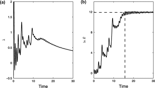
Figure 1 shows the variation of and the logarithm of as a function of time and with an initial magnitude of ∈ = 10⁻⁴. It can be seen that oscillates between positive and negative values at the beginning of the evolution. This is due to the transient error growth period, when errors of random directions align to the fastest growing mode (Trevisan and Legnani 1995). Afterwards, the value fluctuates around a positive value and finally approaches zero as time increases (Figure 1(a)). Correspondingly, the relative error growth saturates to a nonlinear fluctuation level after a period of zigzag growth (Figure 1(b)). The local predictability limit is approximately 16 dimensionless time units.

Figure 1. Temporal evolution of the (a) nonlinear local Lyapunov exponent and (b) logarithm of for the initial state x(−4.87, −7.35, 18.68) on the Lorenz attractor.

Note: The horizontal and vertical dashed lines in (b) are the saturation value of error growth and the local predictability limit, respectively.

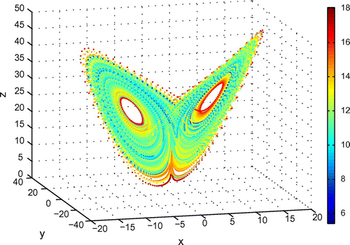
Repeating this procedure over the Lorenz attractor, the distribution of the local predictability limit can be presented quantitatively in the phase space (Figure 2). On the whole, the inner and outer rims of each lobe show a higher local predictability limit, while for the center of each lobe the local predictability limit is lower. This result is quite different from that reported by Nese (1989), but corresponds well with Li et al. (2012), who estimated the predictability limit using space entropy. The reason behind this is the measure of the predictability limit adopted in each study. What Nese (1989) was trying to investigate was the local divergence rate of the linear error growth period. However, the nonlinear error growth dynamics are most prominent after the linear error growth. Only considering the linear error growth makes it impossible to reflect the overall predictability limit. The other characteristic of chaotic systems is the phenomenon of ‘isolated islands’, where nearby points in the phase space may be quite different in the local predictability limit. This is closely related to the sensitivity to the initial conditions of chaotic systems.

Figure 2. The phase-space structure of the local predictability limit over the Lorenz attractor (5 × 10⁴ initial states are chosen in the phase space).

Nese (1989) constructed a Poincare section of the Lorenz-63 attractor by intersecting a trajectory with the plane x = −9. He found that the local divergence rates for the lower piece of the map were always large and positive, while most of the local divergence rates for the upper piece were negative. Thus, he concluded that the predictability is organized, and it is low (high) on the lower (upper) curve. However, Figure 3(a) shows that there are no obvious differences between the distribution of the local predictability limit on the lower and upper curves. Both curves show a higher local predictability limit at both ends but a lower limit in the central parts. The average values of the local predictability limit on the upper and lower curves are 11.4 and 11.7, respectively. Furthermore, the probability distributions are given in Figure 3(b). The difference between the two probability distributions can be measured by the Kullback–Leibler (KL) divergence (Kullback and Leibler 1951). For probability distributions P and Q of a discrete random variable, the KL divergence D_KL (P||Q) of Q from P is calculated by(2)

Figure 3. (a) Intersection of a trajectory on the Lorenz attractor with the Poincare section plane x = −9, where colors indicate the local predictability limit. The lower curve denotes , while the upper one means . (b) Probability density function (PDF) of the intersection points on the lower (blue) and upper (red) curves.

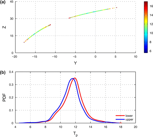
The KL divergence between the probability distributions of the lower and upper curves is 0.0065, which means that the distributions have little difference. This result indicates that the results from the short-term local divergence rate and the long-term local predictability limit are different.

As already known, the fixed points of Equation (1(1) ) are O(0, 0, 0) and , where (Lorenz 1963; Mittal, Dwivedi, and Pandey 2005). For parameters σ = 10, r = 28, b = 8/3, unstable fixed points on the warm regime and the cold regime are and , respectively. Next, we calculate the Euclidean distance between each point and its corresponding fixed point. For a point , the distance R is calculated by(3)

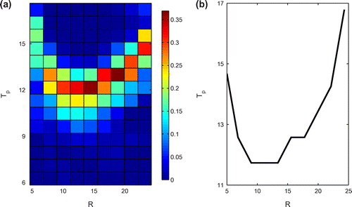
where is the fixed point in its existing regime. Then, we divide R into several intervals. Afterwards, the probability distributions of the local predictability limit in each interval of R are estimated (Figure 4(a)). Clearly, in each interval, the probability of the local predictability limit is nonuniformly distributed. This indicates that the spatial structure of the local predictability limit is quite complex. By taking out the local predictability limit with maximum probability in each interval, a single curve can be drawn, as shown in Figure 4(b). The parabolic shape of the curve indicates that the points are likely to have long predictability limits in the inner and outer rims of both wings on the attractor. Meanwhile, the local predictability limit for the central parts of each regime is prone to be low.

Figure 4. (a) Probability density function (PDF) of the local predictability limit T_p of the Lorenz attractor with respect to each interval of the distance R. (b) The local predictability limit T_p of the Lorenz attractor with the maximum PDF as a function of the distance R.

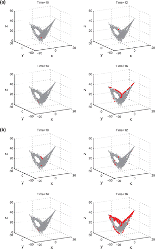
The evolutions of two different points in the phase space are investigated to study the error growth dynamics. One point, P_L(9.24, 6.79, 30.76), has a relatively long local predictability limit of approximately 16, while the other point, P_S(−11.57, −20.58, 16.74), is shorter. P_L is chosen from the inner rim of the warm regime, while P_S is in the central part from the cold regime. For each initial point, 500 different perturbations in random directions with magnitude of 10⁻⁴ are superimposed. Sections of evolutionary trajectories at t = 10, 12, 14, and 16, are shown in Figure 5. As the model evolves, the hypersphere of the initial perturbations begins to deform and stretch into an ellipsoid. At the same time, the directions of the initial errors align to the leading Lyapunov vector, corresponding to the unstable period of the NLLE (Trevisan and Pancotti 1998). Gradually, the information of the initial field is lost (Li and Chou 1997). The ellipsoid is stretched and folded repeatedly, due to the nonlinear effects, until it evolves into an infinitely fractal structure (Kalnay 2002). For the point with shorter predictability, the time at which the nonlinear effects begin to dominate is earlier.

Figure 5. Phase-space evolution of an ensemble of initial errors from (a) the point P_L(9.24, 6.79, 30.76) and (b) the point P_S(−11.57, −20.58, 16.74), at the dimensionless time of 10, 12, 14, and 16, respectively.

Note: The attractor is plotted in gray for reference.

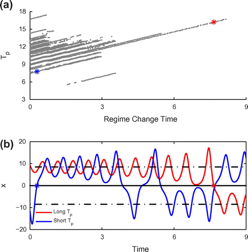
As previously noted (Evans et al. 2004; Zhang, Ide, and Kalnay 2015), the duration in the current regime is critical in determining the predictability limit of each point. As can be seen in Figure 6(a), there seems to be a linear relationship between the time for a point shifting its existing regime and its local predictability limit. The change of regime is affirmed when variables x and y change their signs synchronously. However, as we can see, the relationship is quite complex. The existing time itself cannot be used as a sole predictor of the local predictability limit. The predictability is also related with the position in the phase space. For the two chosen points P_L and P_S, the existing time is 8 and 0.5, respectively (Figure 6(b)). The trajectory oscillates around the unstable fixed point and behaves in a quasi-periodic manner after leaving P_L. Meanwhile, the spiral divergence from as the circuit becomes larger before the trajectory finally shifts to the cold regime after around 8 time units. However, the regime shifts to the warm regime soon after the trajectory leaves P_S in the central part of the cold regime. From this, we conclude that, for the inner and outer rims of each regime, it is easier for the trajectory to oscillate around the unstable fixed points, thus leading to a longer existing time and, ultimately, a longer predictability limit. However, for the central parts in the phase space, the trajectories are prone to shifting from their existing regimes to the other regime. So, the local predictability limit for these points is lower.

Figure 6. (a) Local predictability limit as a function of the residence time in the current regime. (b) Numerical solutions of the Lorenz-63 system for variable x with starting points as P_L (red line) and P_S (blue line), respectively.

Notes: Asterisks denote the regime change time for each point. The upper (lower) dot-dashed line denotes the x-value of the fixed point in the warm (cold) regime.

4. Conclusion

The NLLE is used in the present study to quantitatively estimate the local predictability limit of the Lorenz attractor. The result is quite different to that derived from linear dynamics. Though the local predictability is not uniformly organized, several statistical properties for the Lorenz attractor exist. On the inner and outer rims of both wings of the Lorenz attractor, the local predictability limit is higher than average, while the center part of the attractor shows a lower local predictability limit. However, initially adjacent points in the phase space may possess quite distinct local predictability limits. This corresponds to the sensitivity to the initial conditions of chaotic systems, which may cause considerable difficulties in making long-term analogue forecasts. The source of the local predictability limit is linked to the local dynamics of the point. The region where the point lies in the phase space and the residence time in the current regime are considered. Further work is needed to investigate the source of the local predictability.

Disclosure statement

No potential conflict of interest was reported by the authors.

Funding

This research was supported by the National Natural Science Foundation of China [grant number 41375110].

References

- Abarbanel, H. D. I., R. Brown, and M. B. Kennel. 1991. “Variation of Lyapunov Exponents on a Strange Attractor.” Journal of Nonlinear Science 1: 175–199.10.1007/BF01209065
- Chen, B. H., J. P. Li, and R. Q. Ding. 2006. “Nonlinear Local Lyapunov Exponent and Atmospheric Predictability Research.” Science in China Series D: Earth Sciences 49: 1111–1120.10.1007/s11430-006-1111-0
- Chou, J. F. 1989. “Predictability of the Atmosphere.” Advances in Atmospheric Sciences 6: 335–346.
- Ding, R. Q., and J. P. Li. 2007. “Nonlinear Finite-time Lyapunov Exponent and Predictability.” Physics Letters A 364: 396–400.10.1016/j.physleta.2006.11.094
- Ding, R. Q., J. P. Li, and K. J. Ha. 2008. “Nonlinear Local Lyapunov Exponent and Quantification of Local Predictability.” Chinese Physics Letters 25: 1919–1922.
- Ding, R. Q., J. P. Li, and K.-H. Seo. 2010. “Predictability of the Madden–Julian Oscillation Estimated Using Observational Data.” Monthly Weather Review 138: 1004–1013.10.1175/2009MWR3082.1
- Ding, R. Q., J. P. Li, and K.-H. Seo. 2011. “Estimate of the Predictability of Boreal Summer and Winter Intraseasonal Oscillations from Observations.” Monthly Weather Review 139: 2421–2438.10.1175/2011MWR3571.1
- Ding, R. Q., J. P. Li, and F. Zheng. 2015. “Estimating the Limit of Decadal-scale Climate Predictability Using Observational Data.” Climate Dynamics 46: 1563–1580.
- Eckmann, J. P., and D. Ruelle. 1985. “Ergodic Theory of Chaos and Strange Attractors.” Reviews of Modern Physics 57: 617–656.10.1103/RevModPhys.57.617
- Evans, E., N. Bhatti, L. Pann, J. Kinney, M. Peña, S. C. Yang, E. Kalnay, and J. Hansen. 2004. “RISE: Undergraduates Find That Regime Changes in Lorenz’s Model Are Predictable.” Bulletin of the American Meteorological Society 85: 520–524.10.1175/BAMS-85-4-520
- Feng, G. L., X. G. Dai, A. H. Wang, and J. F. Chou. 2001. “The Study of the Predictability in Chaotic Systems.” Acta Physica Sinica (in Chinese) 50 (4): 606–611.
- He, W. P., G. L. Feng, W. J. Dong, and J. P. Li. 2006. “On the Predictability of the Lorenz System.” Acta Physica Sinica (in Chinese) 55 (2): 969–977.
- Kalnay, E. 2002. Atmospheric Modeling, Data Assimilation and Predictability. New York: Cambridge University Press.10.1017/CBO9780511802270
- Kullback, S., and R. A. Leibler. 1951. “On Information and Sufficiency.” The Annals of Mathematical Statistics 22: 79–86.10.1214/aoms/1177729694
- Li, J. P., and J. F. Chou. 1997. “Existence of the Atmosphere Attractor.” Science in China Series D: Earth Sciences 40: 215–220.10.1007/BF02878381
- Li, J. P., and R. Q. Ding. 2011. “Temporal–spatial Distribution of Atmospheric Predictability Limit by Local Dynamical Analogs.” Monthly Weather Review 139: 3265–3283.10.1175/MWR-D-10-05020.1
- Li, J. P., and R. Q. Ding. 2013. “Temporal-spatial Distribution of the Predictability Limit of Monthly Sea Surface Temperature in the Global Oceans.” International Journal of Climatology 33: 1936–1947.10.1002/joc.2013.33.issue-8
- Li, A. B., L. F. Zhang, Q. L. Wang, B. Li, Z. Z. Li, and Y. Q. Wang. 2012. “Information Theory in Nonlinear Error Growth Dynamics and Its Application to Predictability: Taking the Lorenz System as an Example.” Science China Earth Sciences 56: 1413–1421.
- Lorenz, E. N. 1963. “Deterministic Nonperiodic Flow.” Journal of the Atmospheric Sciences 20: 130–141.10.1175/1520-0469(1963)020<0130:DNF>2.0.CO;2
- Lorenz, E. N. 1965. “A Study of the Predictability of a 28-Variable Atmospheric Model.” Tellus 17: 321–333.
- Lorenz, E. N. 1969a. “Atmospheric Predictability as Revealed by Naturally Occurring Analogues.” Journal of the Atmospheric Sciences 26: 636–646.10.1175/1520-0469(1969)26<636:APARBN>2.0.CO;2
- Lorenz, E. N. 1969b. “The Predictability of a Flow Which Possesses Many Scales of Motion.” Tellus 21: 289–307.
- Mittal, A. K., S. Dwivedi, and A. C. Pandey. 2005. “Bifurcation Analysis of a Paradigmatic Model of Monsoon Prediction.” Nonlinear Processes in Geophysics 12: 707–715.10.5194/npg-12-707-2005
- Mu, M., W. S. Duan, and J. C. Wang. 2002. “The Predictability Problems in Numerical Weather and Climate Prediction.” Advances in Atmospheric Sciences 19: 191–204.10.1007/s00376-002-0016-x
- Mukougawa, H., M. Kimoto, and S. Yoden. 1991. “A Relationship between Local Error Growth and Quasi-stationary States: Case Study in the Lorenz System.” Journal of the Atmospheric Sciences 48: 1231–1237.10.1175/1520-0469(1991)048<1231:ARBLEG>2.0.CO;2
- Nese, J. M. 1989. “Quantifying Local Predictability in Phase Space.” Physica D: Nonlinear Phenomena 35: 237–250.10.1016/0167-2789(89)90105-X
- Sano, M., and Y. Sawada. 1985. “Measurement of the Lyapunov Spectrum from a Chaotic Time Series.” Physical Review Letters 55: 1082–1085.10.1103/PhysRevLett.55.1082
- Thompson, P. D. 1957. “Uncertainty of Initial State as a Factor in the Predictability of Large Scale Atmospheric Flow Patterns.” Tellus 9: 275–295.10.1111/tus.1957.9.issue-3
- Trevisan, A., and R. Legnani. 1995. “Transient Error Growth and Local Predictability: A Study in the Lorenz System.” Tellus A: Dynamic Meteorology and Oceanography 47: 103–117.10.3402/tellusa.v47i1.11496
- Trevisan, A., and F. Pancotti. 1998. “Periodic Orbits, Lyapunov Vectors, and Singular Vectors in the Lorenz System.” Journal of the Atmospheric Sciences 55: 390–398.10.1175/1520-0469(1998)055<0390:POLVAS>2.0.CO;2
- Wang, P. F., J. P. Li, R. Q. Ding, and R. H. Huang. 2012. “Studies of the Attractor Property of Error Equations for the Lorenz System.” Climatic and Environmental Research (in Chinese) 17 (5): 574–582.
- Wolf, A., J. B. Swift, H. L. Swinney, and J. A. Vastano. 1985. “Determining Lyapunov Exponents from a Time Series.” Physica D: Nonlinear Phenomena 16: 285–317.10.1016/0167-2789(85)90011-9
- Yoden, S., and M. Nomura. 1993. “Finite-time Lyapunov Stability Analysis and Its Application to Atmospheric Predictability.” Journal of the Atmospheric Sciences 50: 1531–1543.10.1175/1520-0469(1993)050<1531:FTLSAA>2.0.CO;2
- Zhang, Y., K. Ide, and E. Kalnay. 2015. “Bred Vectors of the Lorenz63 System.” Advances in Atmospheric Sciences 32: 1533–1538.10.1007/s00376-015-4275-8