Cloud vertical structures associated with precipitation magnitudes over the Tibetan Plateau and its neighboring regions

Abstract

Cloud vertical structures and precipitation over the Tibetan Plateau (TP) are analyzed and compared with its neighboring land and tropical oceans based on CloudSat/CALIPSO satellite measurements and TRMM precipitation data. Results show that the TP generally has a compression effect on cloud systems, as manifested by a shrinking cloud depth and lowering cloud top. Precipitation is weaker over the TP than its neighboring regions and exhibits large seasonal variations. In summer, cloud ice particles over the TP are mostly located at lower altitude (5–10 km), with a larger variability of sizes and aggregation (particle number concentration) under no-rain conditions compared to other regions. Ice water content becomes abundant and the number concentration tends to be dense at higher altitudes when precipitation is enhanced. However, even for heavy rainstorms, the aggregation is most likely between 100 and 250 L⁻¹, whereas it can reach as high as 500 L⁻¹ over its neighboring land and tropical oceans. Given the same magnitude of precipitation, the spectrum of ice particle sizes is found to be wider over the TP than other regions.

摘要

本文采用CloudSat/CALIPSO和TRMM卫星资料，对比分析了不同强度降水时青藏高原与其邻近陆地和海洋地区的云宏观和微观垂直结构。结果表明：高原大地形对云层厚度和云顶高度具有压缩效应；与邻近地区相比，高原降水强度较弱，但是季节变化更明显；夏季，无雨时，高原上云冰粒子主要位于较低高度（5-10公里），粒子尺寸和数浓度更丰富；随着降水增强，云冰含量增多，高层冰粒子的聚集度趋于紧密；然而即使是大暴雨，高原地区冰粒子的数浓度也最有可能在100-250 L⁻¹之间，小于其邻近的陆地和热带海洋地区；此外，对于同等级的降水，高原地区冰粒子尺寸的谱分布宽于其它地区。

Keywords:

• CloudSat/CALIPSO
• cloud macrophysics
• cloud microphysics
• cloud vertical structures, precipitation
• Tibetan Plateau

关键词:

• CloudSat/CALIPSO
• 云宏观特征
• 云微物理特征
• 云垂直结构
• 降水
• 青藏高原

1. Introduction

Clouds play a pivotal role in modulating the global radiation budget through reflection of solar radiation and absorption of thermal radiance (Ramanathan et al. 1989; Li, Barker, and Moreau 1995; Kubar, Hartmann, and Wood 2009). However, clouds remain one of the key sources of uncertainty in climate modeling (Dufresne and Bony 2008; Zelinka et al. 2013). One reason is that cloud vertical structures and its microphysical processes are poorly represented (Zhang et al. 2005; Jiang et al. 2012). As an intermediate link between water vapor evaporation and condensation, the effect of cloud on the water cycle is related to both cloud microphysical characteristics and cloud macroscopic characteristics (Charlson et al. 1987). Moreover, cloud vertical structures particularly affect the occurrence and intensity of precipitation (Jakob and Klein 1999). The Tibetan Plateau (TP) significantly affects the atmospheric circulation and climate of Asia through its dynamic and thermal forcing (Wu and Zhang 1998; Duan and Wu 2005; Liu et al. 2007). The transformation process between clouds and precipitation has considerable effects on manipulating atmospheric heating profiles and generating plateau-scale uplifting force, which is a major forcing for establishing and maintaining the TP monsoon circulation (Kuo and Qian 1981). Therefore, exploring cloud vertical structures and its relationship with precipitation over the TP is not only beneficial to further understanding the complexity of the climate system over the plateau, but also helpful in improving the representation of the moist processes that modulate the distribution and variability of clouds and precipitation in numerical models over the TP.

Many studies have investigated the characteristics of cloud over the TP, especially following the advent of satellite-based passive remote sensing (e.g. Fujinami and Yasunari 2001; Kurosaki and Kimura 2002; Chen and Liu 2005; Li, Liu, and Chen 2006; Fu, Li, and Zi 2007). The launch of the CloudSat satellite (Stephens et al. 2002) carrying cloud profile radar, and the CALIPSO satellite (Winker, Hunt, and McGill 2007) carrying the Cloud–Aerosol Lidar with Orthogonal Polarization, in 2006, by NASA, provides an unprecedented opportunity to explore cloud internal properties and vertical structures based on active sensors. Based on CloudSat/CALIPSO products, previous studies have analyzed the vertical structures of cloud microphysical and macrophysical properties over the TP (Wang et al. 2010; Luo, Zhang, and Qian 2011; Rüthrich et al. 2013; Chen and Zhou 2015; Hong and Liu 2015), as well as the relationship between cloud vertical properties and precipitation (Yin, Wang, and Zhai 2011; Zhao, Wang, and Yin 2014). However, little attention has been paid to cloud vertical structures at different precipitation magnitudes.

In operational forecasting, precipitation strength is categorized into light rain (0–10 mm d⁻¹), moderate rain (10–25 mm d⁻¹), heavy rain (25–50 mm d⁻¹), rainstorms (50–100 mm d⁻¹) and heavy rainstorms (>100 mm d⁻¹). But what are the corresponding characteristics of cloud macro- and microphysics in the vertical direction? In this paper, we aim to understand the nature of cloud vertical structures over the TP in association with the precipitation magnitudes used in operational forecasting. For comparison, the TP’s neighboring regions, which we refer to as NIST (northern India and south of the Tibetan Plateau) and TO (tropical ocean), are also analyzed. Following Yan, Liu, and Lu (2016), the three areas are defined as follows: TP (27°–40°N, 70°–103°E; altitude >3000 m); NIST (20°–27°N, 70°–103°E); and TO (20S°–20°N, 60°–150°E; over ocean only).

The rest of the paper is organized as follows: Section 2 describes the data and methodology. Section 3 presents the relationship between cloud macrophysical structures and precipitation, as well as the spectral distribution of cloud vertical microphysics in terms of different precipitation magnitudes. Section 4 presents our conclusions and offers additional discussion.

2. Data and methodology

Two datasets (2B-CWC-RO and 2B-CLDCLASS-LIDAR) (Stephens et al. 2002; 2008), from January 2007 to December 2010, obtained by CloudSat/CALIPSO, are used in this study. The periods when the products failed to provide retrievals are excluded from the diagnostics (Table 1). The 2B-CWC-RO product retrieves estimates of cloud water content, particle effective radius, and number concentration in liquid or ice phase. The portion of the profile colder than −20 °C is deemed to be pure ice, and warmer than 0 °C pure liquid. When the temperature is between 0 °C and −20 °C, the ice and liquid solutions are scaled linearly with temperature by adjusting their particle number concentrations (Austin 2007). Based on this product, GCMs have been evaluated (Su et al. 2011), revealing that models underestimate ice water content in the upper troposphere. Cloud radar has proven to be a highly valuable tool for studies on rainfall and thick precipitating clouds (Matrosov 2007). It has been found that cloud radar can accurately sense between −28 and 6 dBZe, and above 6 dBZe with uncertainties of ±50% (Heymsfield et al. 2008). Thus, especially for heavy rainstorm conditions, the uncertainties in satellite data should be kept in mind. The 2B-CLDCLASS-LIDAR product identifies each cloud detected as one of the eight cloud types (cumulus, stratocumulus, stratus, altocumulus, altostratus, nimbostratus, cirrus, and deep convective cloud), and provides cloud-top height and cloud-base height (Sassen and Wang 2008).

Table 1. The periods when the products failed to provide retrievals.

Product	Year	Periods (Julian Days)
2B-CWC-RO	2007	77–79, 103–105, 111, 128, 157
	2008	19–21, 38, 144–148
	2009	45, 58, 76, 342–365
	2010	1–15, 41, 54
2B-CLDCLASS-LIDAR	2007	16, 77–79, 103–105, 115, 178, 193, 206–208, 289–292, 336, 344, 346, 350–351, 354
	2008	16, 19–21, 63–67, 144–148, 156–161, 199, 201–203, 242–256, 269–270, 272–275
	2009	24–29, 48–75, 163–165, 335–365
	2010	1–15, 153–159, 186, 200, 215–217, 227, 365

We use the same period of three-hourly precipitation data from TRMM 3B42 (Version 6 (Huffman et al. 2007) with a horizontal resolution of 0.25 × 0.25°), together with the CloudSat/CALIPSO datasets, to calculate the relationship between cloud vertical structures and precipitation. This TRMM product has been shown to agree well with gauge measurements and have a weak dependence on topography over the TP (Gao and Liu 2013; Tong et al. 2014). It should be clarified that original orbital profile data (horizontal resolution: ~1.3 km in the across-track direction and ~1.1 km in the along-track direction; vertical resolution: ~240 m) from the 2B-CLDCLASS-LIDAR and 2B-CWC-RO products are used in this study. The sorting method to match the CloudSat/CALIPSO orbital data and TRMM grid data is similar to that used by Yan, Liu, and Lu (2016), which ensures the cloud and precipitation to be almost synchronous (sorted within 1.5 h in the spatial range of 12.5 × 12.5 km). In this study, we define the precipitation rate bins in 10 mm d⁻¹ intervals. In total, 26 bins from 0 mm d⁻¹ to 260 mm d⁻¹, and 1 bin greater than 260 mm d⁻¹, are used, which can provide an intuitive reference for operational forecasting. The joint probability distribution functions (PDFs) are only calculated over precipitating samples, to facilitate comparison of the three regions. The height above sea surface level is used in the analysis.

3. Results

3.1. Cloud vertical macrophysical structures

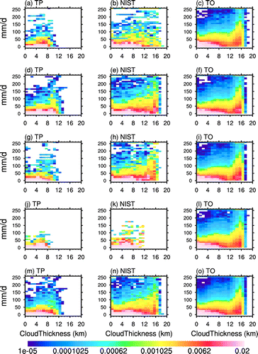
Figure 1 indicates that the TP’s terrain has a compression effect on both precipitation intensity and cloud total thickness (with the clear-sky thickness between adjacent cloud layers deducted). Given that cirrus cloud has little effect on precipitation and may be advected from other regions, it is excluded in the diagnosis. It is found that, even in summer, when precipitation most likely occurs, the main magnitude of precipitation is light, moderate or heavy, while the occurrence of rainstorms or greater magnitude on the plateau is much less than for other regions (Figure 1(d)), which is consistent with the findings of Pan and Fu (2015). The likely reason for this is the restriction of moisture transport caused by high terrain. By calculating the vertically integrated water vapor transport, Zhang (2001) and Yan, Liu, and Lu (2016) found that the abundant water vapor transported from the Indian Ocean is consumed mostly over the southern slopes of the Himalaya. In July, the average divergence of the vertically integrated moisture flux over the three regions is 0.18, −0.59 and −0.08 (units: 10⁻⁴ kg s⁻¹ m⁻²), respectively. In addition, in summer, the total cloud thickness is 0–12 km over the TP when precipitation is smaller than 50 mm d⁻¹, contrasting to 0–16 km over NIST and TO. It is a common feature that clouds thicken with an increase in precipitation magnitude when precipitation is greater than 50 mm d⁻¹. The dominant thickness is 8–12 km over the TP — far thinner compared with the other regions (12–17 km over NIST and TO) (Figure 1(d–f)), demonstrating the limitation imposed by the plateau on the vertical expansion of precipitating clouds.

Figure 1. Probability distribution function of precipitation intensity and total cloud thickness for (a–c) spring (March–May), (d–f) summer (June–August), (g–i) autumn (September–November), (j–l) winter (December–February), and (m–o) the annual mean.

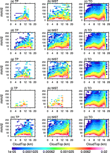
The PDF of precipitation intensity and cloud-top height (Figure 2) further illustrates the suppression effect of the plateau’s topography on precipitation intensity and cloud vertical expansion. When moderate or heavy rain occurs, the main range of cloud-top height over the TP is 4–17 km, indicating that precipitation over the TP during summer is mainly due to shallow convection — consistent with Fu and Liu (2007). While the cloud-top height between 12 and 18 km over TO is more frequent for any precipitation magnitude, combined with the distribution of total cloud thickness (Figure 1), it is clear that more frequent deep convection occurs over TO. The cloud-top height above 18 km over TO in all four seasons, and over NIST in the warm seasons, is related to the activities of overshooting convection (Jensen, Ackerman, and Smith 2007). The variational range of cloud-top height associated with a certain precipitation magnitude shows visible seasonal variation over the TP. For example, when heavy rainstorms occur in spring, the cloud-top height is around 12 km and with a narrow variational range (Figure 2(a)), whereas the top height increases and the variational range expands to 12–18 km in summer, demonstrating strong seasonal variation of cloud vertical structures associated with precipitation magnitudes over the TP.

Figure 2. Probability distribution function of precipitation intensity and cloud top height for (a–c) spring (March–May), (d–f) summer (June–August), (g–i) autumn (September–November), (j–l) winter (December–February), and (m–o) the annual mean.

3.2. Cloud vertical microphysical structures

We focus on the primary rainfall season, summer (June–August), to analyze the vertical distributions of cloud microphysics corresponding to different precipitation magnitudes. Taking into account that the presence of precipitation causes large uncertainty in liquid water inversion (Austin 2007), the features of the liquid phase are not given.

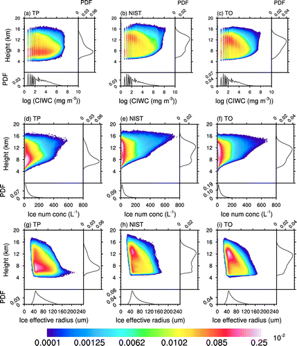
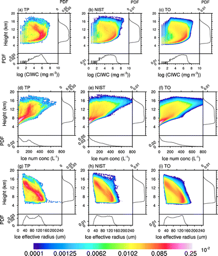
Figure 3 shows the normalized frequency by altitude diagram of cloud ice microphysics for no-rain conditions. In total, there are 566 006, 465 134, and 6 087 019 profiles over the TP, NIST, and TO, respectively. The cloud ice particles are mainly concentrated within 5–10 km, wherein lies the maximum frequency of radar reflectivity (Zhao, Wang, and Yin 2014). The height with maximum probability of cloud ice water content (CIWC) is 7.5 km over the TP, 13 km over NIST, and 12 km over TO, as shown by the curve’s peak on the right-hand side of each plot. Large number concentrations (i.e. >400 L⁻¹) of ice particles are less likely to occur in upper layers of the troposphere (higher than 10 km) over the TP, while moderate values of ice number concentration (<200 L⁻¹) occur more frequently in the whole vertical column compared with other regions (Figure 3(d–f)). Moreover, ice particles distribute over a wider spectrum in lower layers (lower than 10 km) over the plateau, and there are even large particles with sizes greater than 160 μm (Figure 3(g)). The normalized frequency by altitude diagram of CIWC and effective radius under no-rain conditions are generally consistent with all-sky conditions (Zhang, Duan, and Shi 2015). This is because, compared with precipitation profile samples, no-rain profile samples are dominant in the multi-year average over broad areas. A wider variety of ice particle sizes (Figure 3(g)) and number concentration (Figure 3(d)) at 5–10 km in the vertical direction makes a plentiful drift of the CIWC value over the TP (Figure 3(a)). In short, cloud ice particles over the TP are mostly located within 5–10 km, with a wide variety of sizes and aggregation, under no-rain conditions, as compared to the other regions. Above 12 km, particles with large number concentrations appear more over NIST and TO than over the TP.

Figure 3. The normalized frequency by (a–c) altitude diagram (color) of CIWC, (d–f) number concentration, and (g–i) effective radius over the TP (left), NIST (middle), and TO (right) under no rain condition in summer. The X-axis bin for (a–c) is 0.1 (the corresponding value of CIWC is e^0.1 mg m⁻³), for (d–f) is 8 L⁻¹, and for (g–i) is 2.5 μm. While Y-axis bin for all the plots is 240 m. The curve on the right side of each plot is PDF on different altitude. While the curve on the bottom of each plot is PDF on different variable values.

When precipitation occurs, the spectrum of large CIWC increases with an increase in rainfall intensity (Figure 4(a–c); Figure 5(a–c)). Moreover, the particles are more inclined to be large in size at low layers, but still small at high layers (Figure 4(g–i); Figure 5(g–i)), and the radius decreases obviously with height (Figure 5(g–i)). Again, the TP shows unique features, reflected as follows: The CIWC is more diverse over the TP than the other two regions at the same rainfall intensity (Figure 4(a–c); Figure 5(a–c)), and the CIWC over the TP is largely concentrated between 4 and 10 km. When rain is heavy (25–50 mm d⁻¹) (8922, 18 525, and 234 938 profiles over the TP, NIST, and TO regions, respectively), the CIWC, as well as the ice number concentration, increases with altitude below 8 km over the TP (Figure 4(a) and (d)). Above 8 km, the CIWC decreases mainly due to the sharp reduction in the ice effective radius, although the probability of a larger number concentration is increased (Figures 3(d) and 4(d)). Despite heavy rain, the maximum probability of the CIWC is still located near 8 km. Large number concentrations (>600 L⁻¹) seldom occur, and ice clouds are more inclined to gather at moderate concentrations (100–250 L⁻¹) above 9 km over the TP compared with the other regions. This also shows that the plateau features a relatively wider range of particle sizes at the same altitude (shown by the red or deeper colors in Figure 4(g–i)).

Figure 4. The normalized frequency by (a–c) altitude diagram (color) of CIWC, (d–f) number concentration, and (g–i) effective radius over the TP (left), NIST (middle) and TO (right) under heavy rain conditions in summer. The X-axis bin for (a–c) is 0.1 (the corresponding value of CIWC is e^0.1 mg m⁻³), for (d–f) is 8 L⁻¹, and for (g–i) is 2.5 μm. While Y-axis bin for all the plots is 240 m. The curve on the right side of each plot is PDF on different altitude. While the curve on the bottom of each plot is PDF on different variable values.

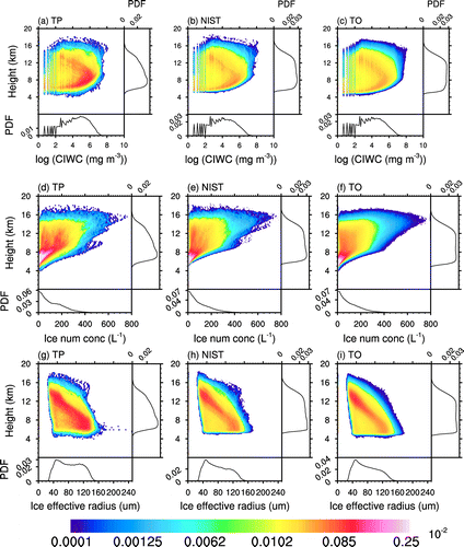
Figure 5. The normalized frequency by (a–c) altitude diagram (color) of CIWC, (d–f) number concentration, and (g–i) effective radius over the TP (left), NIST (middle) and TO (right) under heavy rainstorm in summer. The X-axis bin for (a–c) is 0.1 (the corresponding value of CIWC is e^0.1 mg m⁻³), for (d–f) is 8 L⁻¹, and for (g–i) is 2.5 μm. While Y-axis bin for all the plots is 240 m. The curve on the right side of each plot is PDF on different altitude. While the curve on the bottom of each plot is PDF on different variable values.

For heavy rainstorms (>100 mm d⁻¹) (1613, 9175, and 91 333 profiles over the TP, NIST, and TO regions respectively), the CIWC, as well as the ice number concentration, corresponding to maximum probability, increase remarkably. For example, in heavy rainstorms, the order of dominant CIWC is e⁶ mg m⁻³ (Figure 5(a)), while it is e⁵ mg m⁻³ during heavy rain, over the TP (Figure 4(a)). Above 9 km, the probability of the ice number concentration being greater than 200 L⁻¹ enlarges too, indicating ice clouds consist of much more abundant particles during heavy rainstorms. However, like heavy rain, the probability of a larger number concentration (i.e. >600 L⁻¹) is still less over the TP than over the other regions (Figure 5(d–f)). The particle sizes over the TP display a remarkable decreasing trend with increased altitude, similar to over TO and NIST. The larger occurrence frequencies (red shades) are narrowed (Figure 5(g)) at the same altitude compared with smaller magnitudes of precipitation (Figure 4(g)) over the TP, suggesting that the more even the sizes of cloud ice particles are, the larger the precipitation magnitude.

4. Conclusions and discussion

Based on CloudSat/CALIPSO satellite measurements and TRMM precipitation data, we analyze the characteristics of cloud vertical macro- and microphysical structures associated with precipitation magnitudes over the TP through comparison with neighboring land and ocean regions. The main conclusions are as follows:

(1)	The precipitation magnitude and cloud total thickness are compressed over the TP. Restrictions of water vapor supply induced by topography lead to a lower probability of the precipitation magnitude being greater than ‘rainstorm’ over the TP.
(2)	Cloud vertical expansion, as well as cloud-top height, for the same magnitude of precipitation, is severely confined over the TP compared with other regions. Also, cloud vertical structures associated with precipitation magnitudes show large seasonal variation over the TP.
(3)	Under no-rain conditions, cloud ice particles over the TP are mostly located at lower altitude (5–10 km), with a wide variety of sizes and aggregation, during summer. With an increase in precipitation magnitude, the CIWC and number concentration at high levels (above 10 km) enhance markedly. The low levels are dominated by large particles (100–140 μm).
(4)	Similar to under no-rain conditions, the vertical distributions of cloud ice microphysics are unique over the TP compared to the other regions, even for the same magnitude of precipitation, including a wider range of particle sizes and more moderate particle number concentrations, but a lower probability of dense aggregation (600 L−1).

The results revealed here provide useful information for the potential relationship between cloud and precipitation. However, due to the limitation of local time sampling by CloudSat/CALIPSO, more precise information on the full diurnal cycle needs to be obtained by combining geostationary satellite measurements and ground-based observations. In addition, since uncertainties related to cloud radar retrievals increase with enhanced radar reflectivity, the results revealed here — especially for heavy rainstorm conditions — need to be verified using other datasets. Separating precipitation into convective and stratiform cases is also helpful to reveal associated cloud structures.

Funding

This study was jointly supported by the National Natural Science Foundation of China [grant number 91637312], [grant number 91437219]; the Key Research Program of Frontier Sciences of CAS, the Third Tibetan Plateau Scientific Experiment [grant number GYHY201406001]; the Science and Technology Development Project of Shanghai Meteorological Bureau [grant number QM201711]; and the Special Program for Applied Research on Super Computation of the NSFC–Guangdong Joint Fund (second phase).

Disclosure statement

No potential conflict of interest was reported by the authors.

Acknowledgements

The authors are greatly appreciative of the discussions with, and suggestions made by, Prof. Jianhua LV, from the School of Atmospheric Sciences, Sun Yat-Sen University, China, which certainly improved the manuscript.

References

- Austin, R. 2007. “Level 2B Radar-Only Cloud Water Content (2B-CWC-RO) Process Description Document.” CloudSat Project Report, 24 pp. http://www.cloudsat.cira.colostate.edu/data-products/level-2b/2b-cwc-ro?term=28.
- Charlson, R. J., J. E. Lovelock, M. O. Andreae, and S. G. Warren. 1987. “Oceanic Phytoplankton, Atmospheric Sulphur, Cloud Albedo and Climate.” Nature 326: 655–661.10.1038/326655a0
- Chen, B., and X. Liu. 2005. “Seasonal Migration of Cirrus Clouds over the Asian Monsoon Regions and the Tibetan Plateau Measured from MODIS/Terra.” Geophysical Research Letters 32: L01804. doi:10.1029/2004GL020868.
- Chen, L., and Y. Zhou. 2015. “Different Physical Properties of Summer Precipitation Clouds over Qinghai Xizang Plateau and Sichuan Basin.” [In Chinese.] Plateau Meteorology 34: 621–632.
- Duan, A. M., and G. X. Wu. 2005. “Role of the Tibetan Plateau Thermal Forcing in the Summer Climate Patterns over Subtropical Asia.” Climate Dynamics 24: 793–807. doi:10.1007/s00382-004-0488-8.
- Dufresne, J.-L., and S. Bony. 2008. “An Assessment of the Primary Sources of Spread of Global Warming Estimates from Coupled Atmosphere–Ocean Models.” Journal of Climate 21: 5135–5144. doi:10.1175/2008JCLI2239.1.
- Fu, Y., and G. Liu. 2007. “Possible Misidentification of Rain Type by TRMM PR over Tibetan Plateau.” Journal of Applied Meteorology and Climatology 46: 667–672. doi:10.1175/jam2484.1.
- Fu, Y.-F., H.-T. Li, and Y. Zi. 2007. “Case Study of Precipitation Cloud Structure Viewed by TRMM Satellite in a Valley of the Tibetan Plateau.” [In Chinese.] Plateau Meteorology 26: 98–106.
- Fujinami, H., and T. Yasunari. 2001. “The Seasonal and Intraseasonal Variability of Diurnal Cloud Activity over the Tibetan Plateau.” Journal of the Meteorological Society of Japan 79: 1207–1227. doi:10.2151/jmsj.79.1207.
- Gao, Y., and M. Liu. 2013. “Evaluation of High-Resolution Satellite Precipitation Products Using Rain Gauge Observations over the Tibetan Plateau.” Hydrology and Earth System Sciences 17: 837–849. doi:10.5194/hess-17-837-2013.
- Heymsfield, A., A. Protat, R. T. Austin, D. Bouniol, R. Hogan, J. Delanoë, H. Okamoto, et al. 2008. “Testing IWC Retrieval Methods Using Radar and Ancillary Measurements with In Situ Data.” Journal of Applied Meteorology and Climatology 47: 135–163. doi:10.1175/2007JAMC1606.1.
- Hong, Y., and G. Liu. 2015. “The Characteristics of Ice Cloud Properties Derived from CloudSat and CALIPSO Measurements.” Journal of Climate 28: 3880–3901. doi:10.1175/JCLI-D-14-00666.1.
- Huffman, G. J., R. F. Adler, D. T. Bolvin, G. Gu, E. J. Nelkin, K. P. Bowman, Y. Hong, E. Stocker, and D. B. Wolff. 2007. “The TRMM Multi-satellite Precipitation Analysis (TMPA): Quasi-Global, Multiyear, Combined-Sensor Precipitation Estimates at Fine Scales.” Journal of Hydrometeorology 8: 38–55. doi:10.1175/jhm560.1.
- Jakob, C., and S. A. Klein. 1999. “The Role of Vertically Varying Cloud Fraction in the Parametrization of Microphysical Processes in the ECMWF Model.” Quarterly Journal of the Royal Meteorological Society 125: 941–965.10.1002/(ISSN)1477-870X
- Jensen, E. J., A. S. Ackerman, and J. A. Smith. 2007. “Can Overshooting Convection Dehydrate the Tropical Tropopause Layer?” Journal of Geophysical Research Atmospheres 112: D11209. doi:10.1029/2006JD007943.
- Jiang, J. H., H. Su, C. Zhai, V. S. Perun, A. D. Genio, L. S. Nazarenko, L. J. Donner, et al. 2012. “Evaluation of Cloud and Water Vapor Simulations in CMIP5 Climate Models Using NASA “a-Train” Satellite Observations.” Journal of Geophysical Research Atmospheres 117: D14105. doi:10.1029/2011JD017237.
- Kubar, T. L., D. L. Hartmann, and R. Wood. 2009. “Understanding the Importance of Microphysics and Macrophysics for Warm Rain in Marine Low Clouds. Part I: Satellite Observations.” Journal of the Atmospheric Sciences 66: 2953–2972. doi:10.1175/2009JAS3071.1.
- Kuo, H. L., and Y. F. Qian. 1981. “Influence of the Tibetian Plateau on Cumulative and Diurnal Changes of Weather and Climate in Summer.” Monthly Weather Review 109 (11): 2337–2356.
- Kurosaki, Y., and F. Kimura. 2002. “Relationship between Topography and Daytime Cloud Activity around Tibetan Plateau.” Journal of the Meteorological Society of Japan 80: 1339–1355.10.2151/jmsj.80.1339
- Li, Z., H. W. Barker, and L. Moreau. 1995. “The Variable Effect of Clouds on Atmospheric Absorption of Solar Radiation.” Nature 376: 486–490.10.1038/376486a0
- Li, Y., X. Liu, and B. Chen. 2006. “Cloud Type Climatology over the Tibetan Plateau: A Comparison of ISCCP and MODIS/TERRA Measurements with Surface Observations.” Geophysical Research Letters 33: L17716. doi:10.1029/2006GL026890.
- Liu, Y., Q. Bao, A. Duan, Z. Qian, and G. Wu. 2007. “Recent Progress in the Impact of the Tibetan Plateau on Climate in China.” Advances in Atmospheric Sciences 24: 1060–1076. doi:10.1007/s00376-007-1060-3.
- Luo, Y., R. Zhang, and W. Qian. 2011. “Intercomparison of Deep Convection over the Tibetan Plateau–Asian Monsoon Region and Subtropical North America in Boreal Summer Using CloudSat/CALIPSO Data.” Journal of Climate 24: 2164–2177. doi:10.1175/2010jcli4032.1.
- Matrosov, S. Y. 2007. “Potential for Attenuation-Based Estimations of Rainfall Rate from CloudSat.” Geophysical Research Letters 34: L05817. doi:10.1029/2006GL029161.
- Pan, X., and Y.-F. Fu. 2015. “Analysis on Climatological Characteristics of Deep and Shallow Precipitation Cloud in Summer over Qinghai-Xizang Plateau.” [In Chinese.] Plateau Meteorology 34: 1191–1203.
- Ramanathan, V., R. D. Cess, E. F. Harrison, P. Minnis, B. R. Barkstrom, E. Ahmad, and D. Hartmann. 1989. “Cloud-Radiative Forcing and Climate: Results from the Earth Radiation Budget Experiment.” Science 243: 57–63. doi:10.1126/science.243.4887.57.
- Rüthrich, F., B. Thies, C. Reudenbach, and J. Bendix. 2013. “Cloud Detection and Analysis on the Tibetan Plateau Using Meteosat and CloudSat.” Journal of Geophysical Research Atmospheres 118: 10,082–10,099. doi:10.1002/jgrd.50790.
- Sassen, K., and Z. Wang. 2008. “Classifying Clouds around the Globe with the CloudSat Radar: 1-Year of Results.” Geophysical Research Letter 35 (L04): 805. doi:10.1029/2007GL032591.
- Stephens, G. L., D. G. Vane, R. J. Boain, G. G. Mace, K. Sassen, Z. Wang, A. J. Illingworth, et al. 2002. “The Cloudsat Mission and the A-Train.” Bulletin of the American Meteorological Society 83: 1771–1790. doi:10.1175/bams-83-12-1771.
- Stephens, G. L., D. G. Vane, S. Tanelli, E. Im, S. Durden, M. Rokey, D. Reinke, et al 2008. “CloudSat Mission: Performance and Early Science after the First Year of Operation.” Journal of Geophysical Research Atmospheres 113: D00A18. doi:10.1029/2008JD009982.
- Su, H., J. H. Jiang, J. Teixeira, A. Gettelman, X. Huang, G. Stephens, D. Vane, and V. S. Peru. 2011. “Comparison of Regime-Sorted Tropical Cloud Profiles Observed by CloudSat with GEOS5 Analyses and Two General Circulation Model Simulations.” Journal of Geophysical Research 116: D09104. doi:10.1029/2010JD014971.
- Tong, K., F. Su, D. Yang, and Z. Hao. 2014. “Evaluation of Satellite Precipitation Retrievals and Their Potential Utilities in Hydrologic Modeling over the Tibetan Plateau.” Journal of Hydrology 519: 423–437. doi:10.1016/j.jhydrol.2014.07.044.
- Wang, S.-J., W.-Y. He, H.-B. Chen, J.-C. Bian, and Z.-H. Wang. 2010. “Statistics of Cloud Height over the Tibetan Plateau and Its Surrounding Region Derived from the CloudSat Data.” Plateau Meteorology (in Chinese) 29: 1–9.
- Winker, D. M., W. H. Hunt, and M. J. McGill. 2007. “Initial Performance Assessment of CALIOP.” Geophysical Research Letters 34: L19803. doi:10.1029/2007gl030135.
- Wu, G. X., and Y. S. Zhang. 1998. “Tibetan Plateau Forcing and the Timing of the Monsoon Onset over South Asia and the South China Sea.” Monthly Weather Review 126: 913–927. doi:10.1175/1520-0493(1998)126<0913:Tpfatt>2.0.Co;2.
- Yan, Y., Y. Liu, and J. Lu. 2016. “Cloud Vertical Structure, Precipitation, and Cloud Radiative Effects over Tibetan Plateau and Its Neighboring Regions.” Journal of Geophysical Research Atmospheres 121: 5864–5877. doi:10.1002/2015JD024591.
- Yin, J., D. Wang, and G. Zhai. 2011. “Long-Term in Situ Measurements of the Cloud-Precipitation Microphysical Properties over East Asia.” Atmospheric Research 102: 206–217. doi:10.1016/j.atmosres.2011.07.002.
- Zelinka, M. D., S. A. Klein, K. E. Taylor, T. Andrews, M. J. Webb, J. M. Gregory, and P. Forster. 2013. “Contributions of Different Cloud Types to Feedbacks and Rapid Adjustments in CMIP5.” Journal of Climate 26: 5007–5027. doi:10.1175/JCLI-D-12-00555.1.
- Zhang, R. H. 2001. “Relations of Water Vapor Transport from Indian Monsoon with That over East Asia and the Summer Rainfall in China.” Advance of Atmosphere Science 18 (5): 1005–1017.
- Zhang, M. H., W. Y. Lin, S. A. Klein, J. T. Bacmeister, S. Bony, R. T. Cederwall, A. D. Delgenio, et al 2005. “Comparing Clouds and Their Seasonal Variations in 10 Atmospheric General Circulation Models with Satellite Measurements.” Journal of Geophysical Research Atmospheres 110: D15S02. doi:10.1029/2004JD005021.
- Zhang, X., K. Duan, and P. Shi. 2015. “Cloud Vertical Profiles from CloudSat Data over the Eastern Tibetan Plateau during Summer.” Chinese Journal of tmospheric Sciences (in Chinese) 39: 1073–1080. doi:10.3878/j.issn.1006-9895.1502.14196.
- Zhao, Y., D. Wang, J. Yin. 2014. “A Study on Cloud Microphysical Characteristics over the Tibetan Plateau Using CloudSat Data.” Journal of Tropical Meteorology (in Chinese) 30: 239–248.