Evaluation of the HadISST1 and NSIDC 1850 onward sea ice datasets with a focus on the Barents-Kara seas

ABSTRACT

In recent years, long-term continuous sea-ice datasets have been developed, and they cover the periods before and after the satellite era. How these datasets differ from one another before the satellite era, and whether one is more reliable than the other, is important but unclear because the sea-ice record before 1979 is sparse and not continuous. In this letter, two sets of sea-ice datasets are evaluated: one is the HadISST1 dataset from the Hadley Centre, and the other is the SIBT1850 (Gridded Monthly Sea Ice Extent and Concentration, from 1850 Onward) dataset from the National Snow and Ice Data Center (NSIDC). In view of its substantial importance for climate, the winter sea ice in the Barents and Kara seas (BKS) is of particular focus. A reconstructed BKS sea-ice extent (SIE) is developed using linear regression from the mean of observed surface air temperature at two adjacent islands, Novaya Zemlya and Franz Josef Land (proxy). One validation illustrates that the proxy is substantially coherent with the BKS sea-ice anomaly in the observations and the CMIP5 (phase 5 of the Coupled Model Intercomparison Project) historical experiments. This result indicates that the proxy is reasonable. Therefore, the establishment of the reconstructed BKS SIE is also reasonable. The evaluation results based on the proxy suggest that the sea-ice concentration prior to the satellite era in the NSIDC dataset is more realistic and reliable than that in the Hadley Centre dataset, and thus is more appropriate for use.

Graphical Abstract

摘要

评估HadISST1和NSIDC 1850 onward 两套海冰数据在巴伦支海和喀拉海的数据质量。近年来发展出覆盖卫星观测前后较长时间的海冰数据。这些数据在卫星观测前彼此之间有怎样的不同，是否一个数据要比另一个数据更可信，是很重要但还不清楚的问题。本文评估了两套海冰数据：一套是Hadley中心的，一套是NSIDC的。考虑到巴伦支海和喀拉海的冬季海冰对气候的重要影响故对其进行评估。用线性回归的方法通过在BKS附近的新地岛和法兰是约瑟夫地群岛上的气温建立一个海冰代用指数。代用指数和BKS的海冰的变化有较好的一致性。基于代用指数的评估表明在卫星观测前，NSIDC海冰数据比哈德莱中心的更真实可信，更适合应用。

KEYWORDS:

• Evaluation
• sea-ice dataset
• NSIDC
• Hadley Centre
• proxy

关键字:

• 评估
• 海冰数据
• 美国冰雪中心
• 哈德莱中心
• 代用指数

1. Introduction

Sea-ice data are of primary importance for understanding climate variability and change. During the past several decades, Arctic warming has been at least twice the global average (Blunden and Arndt 2012). One crucial factor for this amplified Arctic warming is the positive feedback between sea-ice reduction and warming. Physically, sea ice not only blocks solar radiation into the upper ocean but also affects the energy and vapor exchange between the atmospheric and oceanic surfaces (He et al. 2018; Li et al. 2018). Furthermore, sea ice plays an important role in midlatitude weather and climate (Yang, Xie, and Huang 1994; Huang and Gao 1999; Wu, Su, and Zhang 2011; Li and Wang 2013; Guo et al. 2014; Gao et al. 2015; Zuo et al. 2016; Wu, Yang, and Francis 2016). However, there are still uncertainties regarding the effect of sea ice on climate, because the strong internal variability of the atmosphere at the mid–high latitudes may obscure the effects of sea ice (Walsh 2014; Overland et al. 2015). To understand the impact of sea ice more thoroughly and reduce the uncertainty, a longer sea-ice dataset is necessary.

However, reliable sea-ice data were unavailable until 1979, when satellite observations began. Thus, various sea-ice datasets were extended back to the 19th century and continued to the 21st century. One of the most often used is the sea-ice concentration dataset from the UK Met Office’s Hadley Centre (HadISST1; Rayner et al. (2003); hereafter, ‘Hadley dataset’). It has a horizontal resolution of 1.0° × 1.0° and a time span from 1870 to the present day. HadISST2 is an updated version of HadISST1, constructed by Titchner and Rayner (2014). Another sea-ice dataset is the Gridded Monthly Sea Ice Extent and Concentration dataset (SIBT1850). This dataset is from the National Snow and Ice Data Center (NSIDC) (Walsh, Chapman, and Fetterer 2015). Although the NSIDC provides a great number of different datasets, in this letter, ‘the NSIDC dataset’ refers to the SIBT1850 dataset. In comparison with the Hadley dataset, the NSIDC dataset has a finer horizontal resolution of 0.25° × 0.25° and spans from 1850 to the end of 2013. Additionally, the dataset has more sources (14 in total), such as whaling ship reports. Every source is represented by a specific number. The method used to merge the data sources is based on a ranking hierarchy, where higher numbers outrank lower ones. Each of the potential sources for a sea-ice concentration value at a particular location is given a rank with a specific number. How these datasets differ from one another, and whether one is more reliable than the other, is important but unclear, because the sea-ice record prior to 1979 is sparse and not continuous. Evaluating the quality of these two datasets constitutes the primary aim of this study.

Evaluation will be conducted only for the period after 1958. This is because, prior to 1958 (the first international geophysical year), atmospheric variables upon which the reconstructed sea-ice extent (SIE) is based had a lack of systematic in-situ observations in the polar regions. Particular attention is given to the two sub-periods before and after the satellite era: 1958–78 and 1979–2013, respectively. Winter sea ice in the Barents and Kara seas (BKS) is studied, because the sea ice in this region is more active and more closely related to climate anomalies (Wu, Huang, and Gao 1999; Sorokina et al. 2016; Wu et al. 2016).

2. Preliminary comparison of sea-ice variability

Before evaluating the two datasets, we conduct a preliminary comparison of their sea-ice variability. Using a bilinear interpolation method, the data obtained from the NSIDC dataset is interpolated from 0.25° × 0.25° into 1° × 1°, which is the same resolution as the Hadley dataset. The SIE is defined as the sum of the area where the sea-ice concentration is above 15% for a separated grid point. Winter refers to December through February; for example, the winter of 1979 refers to December 1978 through February 1979.

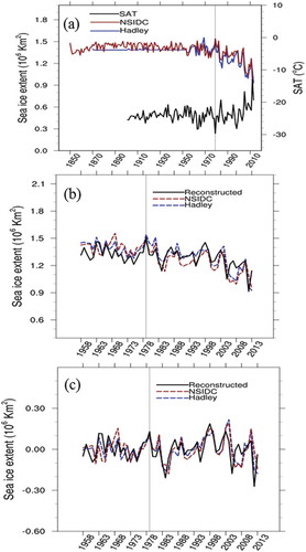
Figure 1 displays the historical evolution of the winter mean BKS SIE. Here, the BKS region refers to the domain shown as the green polygon in Figure 2(e) (70.5°–81.5°N, 15.5°–90.5°E). For the period of 1958–2013, the two datasets are overall consistent (Figure 1), with a high correlation coefficient of 0.91 (Table 1). This consistency is also observed in their standard deviation (not shown). However, when the period is separated into two sub-periods, before and after 1979, there are obvious differences between the two datasets.

Table 1. Correlation coefficients of winter BKS SIE between the Hadley and NSIDC datasets for three periods. Bracketed is the result after detrending.

Period	Correlation coefficients
1958–78	0.64 (0.72)
1979–2013	0.95 (0.92)
1958–2013	0.91 (0.81)

Figure 1. Time series of winter BKS SIE. The maroon curve is for the NSIDC dataset and the blue curve is for the Hadley dataset. The first year of the satellite era, 1979, is marked with the vertical black line.

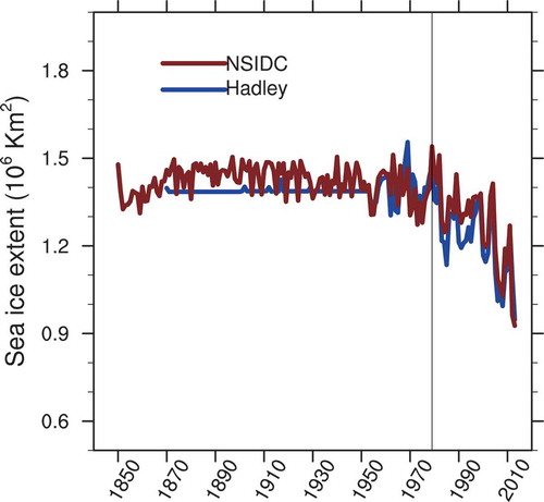
Figure 2. (a) Standard deviation of the winter sea-ice concentration calculated for the period 1979–2013 with the Hadley data. (b) As in (a) but for the NSIDC data. (c) Difference between (a) and (b). (d–f) As in (a–c) but for the period 1958–1978. We defined the green polygon in (e) as the BKS area; the yellow polygon is the area we used to calculate the domain-averaged SAT over Novaya Zemlya and Franz Josef Land.

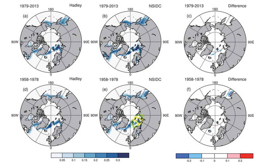
For the satellite era after 1979, the consistency between the two datasets is most evident. From the interannual evolution of BKS SIE (Figure 1), the two datasets share the same years with more (less) sea ice in 2006 and 2010 (2007 and 2012). This high consistency is emphasized by the high correlation coefficient (0.95, Table 1). The standard deviation (Figure 2(a,b)) displays similar maxima in sea-ice interannual variability in the BKS, Greenland Sea, Labrador Sea, Bering Sea and Okhotsk Sea.

For the period 1958–78, the consistency reduces substantially. First, the correlation coefficient in BKS SIE between the two datasets reduces to 0.64 from 0.95 (Table 1). Second, the standard deviation of the winter monthly sea ice in the Northern Hemisphere exhibits a visually distinct difference over the Okhotsk Sea. This observation suggests a difference and uncertainty between the two datasets for the period prior to 1979. To exclude the potential contribution from the linear trend, we recalculated the correlation of BKS SIE for the detrended data and found the same result. Thus, the difference between the two datasets during the period prior to 1979 is not a result of the different trends in the datasets.

3. Proxy for BKS sea ice

In the above section we illustrate the inconsistency in BKS sea-ice variability prior to 1979 between the two datasets. Which dataset is more reliable is an important issue. Here, we develop a reconstructed SIE based on the idea that the sea-ice variation in BKS is not isolated but closely related to surface air temperature (SAT) at adjacent islands. Also, the SAT record over land has a much longer time span and greater reliability.

First, sea ice is impacted by atmospheric circulation. It also has feedbacks on the atmosphere inducing the SAT anomaly over the adjacent regions (Sorteberg and Kvingedal 2006; Deser and Teng 2008; Zhang et al. 2008; Overland, Wood, and Wang 2011; Wu, Overland, and D’Arrigo 2012; Luo et al. 2016). In other words, a correlation exists between sea ice and the SAT anomaly in the ice–atmospheric interaction regions. Second, oceanic flow processes can also cause a correlation between the sea ice and the overlying atmosphere. For example, the sea-ice anomaly can act on the overlying atmosphere in a larger domain because of its larger heat content and longer persistence relative to the atmosphere (Wu et al. 2013), and the oceanic heat transport influencing sea-ice variation usually leads to warmer SAT over adjacent lands (Schlichtholz 2011; Pavlova, Pavlov, and Gerland 2014). The correlation of sea ice with SAT in adjacent lands provides a physical basis for using adjacent land SAT as a proxy of sea ice.

In Figure 3, simultaneous correlations between the winter BKS SIE and some atmospheric variables after 1979 are shown. Here, the BKS SIE is derived from the NSIDC data. Also, the SAT is from the version 3.24.01 time series of the Climatic Research Unit (CRU), University of East Anglia, UK (University of East Anglia Climatic Research Unit, I. C. Harris, P. D. Jones 2017), which has a horizontal resolution of 0.5° × 0.5° and a time span of 1900 through 2015. The 10-m above ground wind, sea level pressure (SLP) and 500-hPa geopotential height (Z500) at 1.25° horizontal resolution are from the JRA-55 dataset (Kobayashi et al. 2015). Figure 3(a) indicates that BKS SIE is substantially negatively correlated with the SAT at the adjacent islands — namely, Novaya Zemlya and Franz Josef Land (yellow polygon in Figure 2(e)). Two factors may explain this negative correlation. First, the SLP anomalies corresponding to increased BKS sea ice are negative (Figure 3(b)), and the anomalous northerly wind in the northwestern region of the anomalous low-pressure zone transports cold polar air southward and induces colder SAT over the islands. The negative Z500 anomaly overlaps with the anomalous low, suggesting a barotropic atmospheric circulation anomaly (Figure 3(c)). A similar connection between BKS sea ice and the Z500 has been observed in previous studies (Luo et al. 2016; Sorokina et al. 2016). Second, the anomalous northerly tends to reduce the climatological surface southerly and causes colder SAT (Figure 3(d)). Therefore, the coherence of BKS sea ice with SAT at the islands of Novaya Zemlya and Franz Josef Land may be physically reasonable.

Figure 3. Correlation of the winter BKS SIE with (a) near-surface air temperature from the CRU data, (b) SLP and surface horizontal wind (black arrows), and (c) Z500 from JRA-55. The period used to calculate the correlation is 1979–2013. Italics indicate significance at the 0.01 level for a two-sided Student’s t-test. For comparison, the climatological winter mean surface wind is also displayed in (d). Units: m s^−1.

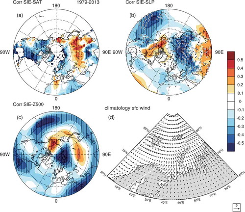
Table 2 shows the high correlation coefficients between BKS SIE and SAT over the Novaya Zemlya and Franz Josef Land after 1979. The coherence of BKS sea ice with SAT over adjacent lands and the physical basis for this coherence is also seen in the historical runs from 21 coupled models (Table 3) involved in phase 5 of the Coupled Model Intercomparison Project (CMIP5). Here, these models are used for analysis because of their availability. Additionally, for a convenient comparison with the observations in the satellite era, 27 years spanning 1979–2005 are used. The multi-model ensemble correlation is calculated based on the extended BKS SIE series by linking the individual model results into one single long series. From Figure S1(a), BKS SIE is negatively correlated with the SAT over the Arctic and Eurasian high latitudes, similar to the observations (Figure 3(a)). The correlation of SLP also bears some similarity to the observations (cf. Figures S1(b) and 3(b)). There is an east–west dipole in the high-latitude region, with negative correlation in Eurasia but positive correlation in North America, although the negative center over the Eurasian high latitudes shifts somewhat southward. The islands mentioned above are governed by the anomalous northerly wind on the east side of the anomalous high extending from eastern North America to Greenland and causing a southward transport of cold polar air that results in a colder SAT. The Z500 anomalies at high latitudes (Figure S1(c)) also appear similar to the observations, although less significant over Eurasia.

Table 2. Correlation coefficients of BKS SIE in the Hadley and NSIDC datasets with the domain-averaged SAT over Novaya Zemlya and Franz Josef Land for three periods. Bracketed is the result after detrending.

	1958–78	1979–2013	1958–2013
Hadley	−0.26 (−0.24)	−0.74 (−0.61)	−0.64 (−0.53)
NSIDC	−0.64 (−0.58)	−0.78 (−0.67)	−0.76 (−0.65)

Table 3. Correlation coefficients between the BKS SIE and the domain-averaged SAT over Novaya Zemlya and Franz Josef Land in CMIP5 models for 1979–2005 and 1960–1978.

No.	Model	1979–2005	1960–1978
1	ACCESS1-3	−0.78	−0.90
2	BCC-CSM1-1	−0.59	−0.52
3	BCC-CSM1-1-M	−0.59	−0.38
4	CCSM4	−0.78	−0.79
5	CESM1-CAM5	−0.73	−0.87
6	CESM1-FASTCHEM	−0.80	−0.88
7	CESM1-WACCM	−0.79	−0.60
8	CNRM-CM5	−0.72	−0.34
9	FGOALS-g2	−0.20	−0.32
10	GFDL-CM3	−0.84	−0.82
11	GISS-E2-H	−0.68	−0.66
12	GISS-E2-R	−0.61	−0.18
13	HadCM3	−0.75	−0.70
14	HadGEM2-ES	−0.92	−0.89
15	IPSL-CM5A-LR	−0.29	0.05
16	MIROC5	−0.86	−0.82
17	MIROC-ESM	−0.89	−0.89
18	MPI-ESM-LR	−0.76	−0.92
19	MPI-ESM-MR	−0.87	−0.92
20	MRI-CGCM3	−0.55	−0.54
21	NorESM1-M	−0.85	−0.72

The above analysis again suggests that the correlation between BKS sea ice and the SAT over Novaya Zemlya and Franz Josef Land is physically reasonable. Thus, the domain-averaged SAT over Novaya Zemlya and Franz Josef Land (70°–82°N, 44°–70°E) can be used as a proxy to reconstruct the BKS SIE. Below, we further verify this point by comparing the proxy with the SIE in the observed dataset and the CMIP5 historical runs.

The winter mean SAT over Novaya Zemlya and Franz Josef Land is calculated from the CRU’s observational global land SAT dataset or the CMIP5 models. Similarly, the BKS SIE can easily be derived. A substantially negative correlation between the BKS SIE and the domain-averaged SAT is seen in the two ice datasets (Table 2) and nearly all of the models (Table 3). The correlation coefficients of the domain-averaged SAT with the BKS SIE in the two observational datasets are −0.74 and −0.78 during the satellite era (1979–2013). Additionally, the correlation coefficients in more than two-thirds of the CMIP5 models (16 of 21 models) is less than −0.6. For 19 models (all models except FGOALS-g2 and IPSL-CM5A-LR), the correlation coefficients are smaller than −0.32, meaning that the models are above the 90% confidence level. When the analysis period for the models is extended backward to 1960, the significant negative correlation in most of the models remains.

Thus, we used the proxy to establish a reconstructed BKS SIE by using linear regression as follows:

(1)

Here, y is the reconstructed BKS SIE, and x is the domain-averaged SAT (proxy). By using least-squares fitting, the coefficients a and b are calculated based on the observed BKS SIE and the proxy during the period 1979–2013, and have the values −0.035 and 0.456, respectively.

As a validation, the SAT-based reconstructed BKS SIE using the regression model is compared with the observed sea ice for 1979–2013. Calculation suggests that the reconstructed SIE correlates well with the SIE in the two datasets, with correlation coefficients of 0.74 and 0.78 (Table 4), respectively. From Figure 4(b), the reconstructed SIE sufficiently captures the variation of the observed SIE. This agreement indicates that the SAT-based reconstructed SIE is an appropriate representation of the sea ice. Because of the greater reliability and the longer time span of the SAT data than those of the sea-ice data prior to 1979, the proxy provides a valuable approach to evaluate the sea ice prior to the satellite era. In the next section, we use the reconstructed SIE as a benchmark to evaluate the sea ice prior to 1979.

Table 4. Correlation coefficients of BKS SIE in the Hadley and NSIDC datasets with the reconstructed SIE for three periods. Bracketed is the result after detrending.

	1958–1978	1979–2013	1958–2013
Hadley	0.26 (0.24)	0.74 (0.61)	0.64 (0.53)
NSIDC	0.64 (0.58)	0.78 (0.67)	0.76 (0.65)

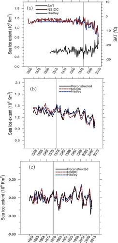
Figure 4. Time series of winter BKS SIE (a) with the overlap of the domain-averaged SAT over Novaya Zemlya and Franz Josef Land; (b) with the reconstructed SIE overlap; (c) after detrending with the reconstructed SIE after detrending overlap. The maroon curve is for the NSIDC dataset, the blue curve is for the Hadley dataset and the black curve is for the CRU SAT. The first year of the satellite era, 1979, is marked with the vertical black line.

4. Evaluation result

Figure 4 compares the BKS SIE in the two datasets with the reconstructed BKS SIE. As seen above, it is unsurprising that the evolution of the SIE prior to 1979 (i.e., 1958–78) in the two sea-ice datasets is different. The BKS SIE in the NSIDC dataset is more strongly correlated with the proxy (−0.64) and the reconstructed SIE (0.64) than the Hadley dataset is (−0.26 and 0.26; Tables 2 and 4). This finding suggests that the quality of the sea-ice data from NSIDC is better than that of the data from Hadley. The lower correlation (0.64) of BKS SIE in the Hadley dataset than that in the NSIDC dataset (0.76) with the reconstructed SIE during the whole period from 1958 to 2013 is in agreement with this assessment. Thus, the interannual BKS sea-ice data in the NSIDC data are relatively more reliable.

The greater reliability of the NSIDC sea-ice data prior to 1979 is consistent with the standard deviation distribution. As mentioned in section 2, the standard deviation for the period before 1979 in the two datasets exhibits a substantial difference, particularly in the Okhotsk Sea (Figure 2(f)). When comparing the sea-ice standard deviation before and after 1979, the NSIDC data before 1979 not only bear a greater resemblance to themselves but also to the Hadley data after 1979. To some extent, this result further verifies the greater reliability of the NSIDC data before 1979.

5. Conclusions and discussion

In this letter, the quality of sea ice in the BKS before 1979 in two datasets, one from the UK’s Hadley Centre and the other from NSIDC, is investigated. The sea-ice proxy is the average mean of winter (December–January–February) SAT over the islands of Novaya Zemlya and Franz Josef Land. Based on the proxy, the reconstructed sea ice is used as a benchmark. The results suggest that the winter BKS sea-ice quality in the NSIDC data is higher than that in the Hadley data for the period 1958–78, although both datasets are substantially consistent with each other and reasonable after 1979. Here, the quality means the interannual variability of the sea ice. The better quality of the dataset from NSIDC may be related to the data source used and the analog method to fill in temporal gaps. By checking the data sources used in the BKS, we found that both the Walsh and Johnson data (source No. 5) and the Russian Arctic and Antarctic Research Institute (AARI) data (source No. 10) had values. According to the ranking method introduced in the introduction, the AARI data are used instead of the Walsh and Johnson data, which are different from the Hadley data. The analog method is used to fill in temporal gaps in the NSIDC dataset. It is possible that the different methods used to fill temporal gaps may also lead to different results.

The impact of the sea ice in BKS on the atmosphere is still controversial and deserves further study (Wu, Su, and D'Arrigo 2015; Walsh 2014; Kelleher and Screen 2018). There is a need for a reliable sea-ice dataset that encompasses a long time period. The present study suggests that the sea ice from NSIDC is more appropriate for such studies.

Semenov and Latif (2015) demonstrated that winter sea-ice concentrations in BKS show an obvious positive bias from 1966–1969 relative to those during 1971–2000 in the Hadley dataset (Figure S2(a)). When a similar comparison for the two periods using the NSIDC dataset is conducted, no evident positive bias is seen (Figure S2(b)). This result suggests that the bias may result from the Hadley dataset itself.

Here, we only choose the SAT at the islands of Novaya Zemlya and Franz Josef Land as the proxy. One may wonder why the SAT over Svalbard is not used, because the SAT there is similarly negatively correlated with the BKS sea ice (Figure 3(a) and S1(a)). There are two arguments for our choice. One is that the climatological southerly component around Novaya Zemlya and Franz Josef Land is stronger, and the SAT over the two islands is influenced more easily by local sea ice, even for the period prior to 1979 when the climatological sea-ice boundary is at a more southern location. The other is that there is less of the sea-ice anomaly east of Svalbard before 1979, and the SAT anomaly caused by the sea ice cannot be easily transported to Svalbard.

Acknowledgments

The CMIP5 historical experiments are supported by the climate modeling groups on the website http://cmip-pcmdi.llnl.gov/cmip5/data_portal.html.

Disclosure statement

No potential conflict of interest was reported by the authors.

Supplementary material

Supplementary data can be accessed here

Additional information

Funding

This work was jointly supported by the National Natural Science Foundation of China [grant numbers 41790473 and 41421004] and the Strategic Priority Research Program of the Chinese Academy of Sciences [grant number XDA19070402].

References

- Blunden, J., and D. S. Arndt. 2012. “State of the Climate in 2011.” Bulletin of the American Meteorology Society 93: S1–S264. Special supplement
- Deser, C., and H. Y. Teng. 2008. “Evolution of Arctic Sea Ice Concentration Trends and the Role of Atmospheric Circulation Forcing 1979–2007.” Geophysical Research Letters 35: L02504. doi:10.1029/2007GL032023.
- Gao, Y. Q., J. Q. Sun, F. Li, S. P. He, S. Sandven, Q. Yan, Z. S. Zhang, et al. 2015. “Arctic Sea Ice and Eurasian Climate: A Review.” Advances in Atmospheric Science 32 (1): 92–114. doi:10.1007/s00376-014-0009-6.
- Guo, D., Y. Q. Gao, I. Bethke, D. Y. Gong, O. M. Johannessen, and H. J. Wang. 2014. “Mechanism on How the Sprin Arctic Sea Ice Impacts the East Asian Summer Monsoon.” Theoretical and Applied Climatology 115: 107–119. doi:10.1007/s00704-013-0872-6.
- He, S. P., Y. Q. Gao, T. Furevik, H. J. Wang, and F. Li. 2018. “Teleconnection between Sea Ice in the Barents Sea in June and the Silk Road, Pacific–Japan and East Asian Rainfall Patterns in August.” Advances in Atmospheric Sciences. doi:10.1007/s00376-017-7029-y.
- Huang, R. H., and D. Y. Gao. 1999. “The Impact of Variation of Sea Ice Extent in the Kara Sea and the Barents Seas in Winter on the Winter Monsoon over East Asia.” Chinese Journal of Atmospheric Science 23 (3): 267–275.
- Kelleher, M., and J. Screen. 2018. “Atmospheric Precursors of and Response to Anomalous Arctic Sea Ice in CMIP5 Models.” Advances in Atmospheric Science 35 (1): 27–37. doi:10.1007/s00376-017-7039-9.
- Kobayashi, S., Y. Ota, Y. Harada, A. Ebita, M. Moriva, H. Onoda, K. Onogi, et al. 2015. ““The JRA-55 Reanalysis: General Specifications and Basic Characteristics.” Journal of the Meteorological Society of Japan 93 :5–48. doi:10.2151/jmsj.2015-001.
- Li, F., Y. J. Orsolini, H. Wang, Y. Gao, and S. He. 2018. “Modulation of the Aleutian–Icelandic Low Seesaw and Its Surface Impacts by the Atlantic Multidecadal Oscillation.” Advances in Atmospheric Sciences 34 (12). doi:10.1007/s00376-017-7028-z.
- Li, F., and H. J. Wang. 2013. “Autumn Sea Ice Cover, Winter Northern Hemisphere Annular Mode, and Winter Precipitation in Eurasia.” Journal of Climate 26 (11): 3968–3981. doi:10.1175/JCLI-D-12-00380.1.
- Luo, D. H., Y. Q. Xiao, Y. Yao, A. G. Dai, I. Simmonds, and C. L. E. Franzke. 2016. “Impact of Ural Blocking on Winter Warm Arctic-Cold Eurasian Anomalies Part I: Blocking-Induced Amplification.” Journal of Climate 29: 3925–3947. doi:10.1175/JCLI-D-15-0611.1.
- Overland, J. E., J. A. Francis, R. Hall, E. Hanna, S.-J. Kim, and T. Vihma. 2015. “The Melting Arctic and Midlatitude Weather Patterns: Are They Connected?” Journal of Climate 28: 7917–7932. doi:10.1175/JCLI-D-14-00822.1.
- Overland, J. E., K. R. Wood, and M. Wang. 2011. “Warm Arctic-Cold Continents: Climate Impacts of the Newly Open Arctic Sea.” Polar Research 30: 15787. doi:10.3402/polar.v30i0.15787.
- Pavlova, O., V. Pavlov, and S. Gerland. 2014. “The Impact of Winds and Sea Surface Temperatures on the Barents Sea Ice Extent, a Statistical Approach.” Journal of Marine Systems 130: 248–255. doi:10.1016/j.jmarsys.2013.02.011.
- Rayner, N. A., D. E. Parker, E. B. Horton, C. K. Folland, L. V. Alexander, D. P. Rowell, E. C. Kent, and A. Kaplan. 2003. “Global Analyses of Sea Surface Temperature, Sea Ice, and Night Marine Air Temperature since the Late Nineteenth Century.” Journal of Geophysical Research 108: 4407–4443. doi:10.1029/2002JD002670.
- Schlichtholz, P. 2011. “Influence of Oceanic Heat Variability on Sea Ice Anomalies in the Nordic Seas.” Geophysical Research Letter 38 (5): 387–404. doi:10.1029/2010GL045894.
- Semenov, V. A., and M. Latif. 2015. “Nonlinear Winter Atmospheric Circulation Response to Arctic Sea Ice Concentration Anomalies for Different Periods during 1966–2012.” Environmental Research Letters 10 (2015): 054020. doi:10.1088/1748-9326/10/5/054020.
- Sorokina, S. A., C. Li, J. J. Wettstein, and N. G. Kvamstø. 2016. “Observed Atmospheric Coupling between Barents Sea Ice and the Warm-Arctic Cold-Siberian Anomaly Pattern.” Journal of Climate 29 (2): 495–511. doi:10.1175/JCLI-D-15-0046.1.
- Sorteberg, A., and B. Kvingedal. 2006. “Atmospheric Forcing on the Barents Sea Winter Ice Extent.” Journal of Climate 19 (19): 4772–4784. doi:10.1175/JCLI3885.1.
- Titchner, H. A., and N. A. Rayner. 2014. “The Met Office Hadley Centre Sea Ice and Sea Surface Temperature Data Set, Version 2: 1. Sea Ice Concentrations.” Journal Geophys Researcher Atmos 119: 2864–2889. doi:10.1002/2013JD020316.
- University of East Anglia Climatic Research Unit, I. C. Harris, P. D. Jones. 2017. CRU TS3.24.01: Climatic Research Unit (CRU) Time-Series (TS) Version 3. 24.01of High Resolution Gridded Data of Month-By-Month Variation in Climate (Jan. 1901- Dec. 2015). Centre for Environmental Data Analysis. Center for Environmental Data Analysis(CEDA). Accessed 25 August 2017. doi:10.5285/3df7562727314bab963282e6a0284f24.
- Walsh, J. E. 2014. “Intensified Warming of the Arctic: Causes and Impacts on Middle Latitudes.” Global Planetary Change 117: 52–63. doi:10.1016/j.gloplacha.2014.03.003.
- Walsh, J. E., W. L. Chapman, and F. Fetterer. 2015. updated 2016. Gridded Monthly Sea Ice Extent and Concentration, 1850 Onwards, Version 1.1. Boulder, Colorado USA: National Snow and Ice Data Center (NSIDC). doi:10.7265/N5833PZ5.
- Wu, B. Y., R. H. Huang, and D. Y. Gao. 1999. “Effects of Variation of Winter Sea Ice Area in Kara and Barents Seas on East Asian Winter Monsoon.” Acta Meteorological Sinica 13: 141–153.
- Wu, B. Y., J. E. Overland, and R. D’Arrigo. 2012. “Anomalous Arctic Surface Wind Patterns and Their Impacts on September Sea Ice Minima and Trend.” Tellus A 64: 18590. doi:10.3402/tellusa.v64i0.18590.
- Wu, B. Y., J. Z. Su, and R. D’Arrigo. 2015. “Patterns of Asian Winter Climate Variability and Links to Arctic Sea Ice.” Journal of Climate 28: 6841–6858. doi:10.1175/JCLI-D-14-00274.1.
- Wu, B. Y., J. Z. Su, and R. H. Zhang. 2011. “Effects of Autumn-Winter Arctic Sea Ice on Winter Siberian High.” Chinese Science Bulletin 56 (30): 3220–3228. doi:10.1007/s11434-011-4696-4.
- Wu, B. Y., K. Yang, and J. A. Francis. 2016. “Summer Arctic Dipole Wind Pattern Affects the Winter Siberian High.” International Journal of Climatology 36: 4187–4201. doi:10.1002/joc.4623.
- Wu, B. Y., R. H. Zhang, R. D’Arrigo, and J. Z. Su. 2013. “On the Relationship between Winter Sea Ice and Summer Atmospheric Circulation over Eurasia.” Journal of Climate 26: 5523–5536. doi:10.1175/JCLI-D-12-00524.1.
- Wu, Z. W., X. Li, Y. J. Li, and Y. Li. 2016. “Potential Influence of Arctic Sea Ice to the Inter-Annual Variations of East Asian Spring Precipitation.” Journal of Climate 29: 2797–2813. doi:10.1175/JCLI-D-15-0128.1.
- Yang, X. Q., Q. Xie, and S. S. Huang. 1994. “Numerical Simulation in the Impact of Arctic Sea Ice Anomaly on the East Asian Summer Monsoon.” Acta Oceanological Sincia 16 (5): 34–40.
- Zhang, X. D., A. Sorteberg, J. Zhang, R. Gerdes, and J. C. Comiso. 2008. “Recent Radical Shifts of Atmospheric Circulations and Rapid Changes in Arctic Climate System.” Geophysical Research Letters 35: L22701. doi:10.1029/2008GL035607.
- Zuo, J. Q., H. L. Ren, B. Y. Wu, and W. J. Li. 2016. “Predictability of Winter Temperature in China from Previous Autumn Arctic Sea Ice.” Climate Dynamics 47: 2331–2343. doi:10.1007/s00382-015-2966-6.