Lower bound estimation of the maximum allowable initial error and its numerical calculation

ABSTRACT

In the numerical prediction of weather or climate events, the uncertainty of the initial values and/or prediction models can bring the forecast result’s uncertainty. Due to the absence of true states, studies on this problem mainly focus on the three subproblems of predictability, i.e., the lower bound of the maximum predictable time, the upper bound of the prediction error, and the lower bound of the maximum allowable initial error. Aimed at the problem of the lower bound estimation of the maximum allowable initial error, this study first illustrates the shortcoming of the existing estimation, and then presents a new estimation based on the initial observation precision and proves it theoretically. Furthermore, the new lower bound estimations of both the two-dimensional ikeda model and lorenz96 model are obtained by using the cnop (conditional nonlinear optimal perturbation) method and a pso (particle swarm optimization) algorithm, and the estimated precisions are also analyzed. Besides, the estimations yielded by the existing and new formulas are compared; the results show that the estimations produced by the existing formula are often incorrect.

Graphical Abstract

摘要

本文基于观测误差限，针对可预报性问题中第三个子问题最大允许初始误差，分析了前人给出的下界估计的不足，给出了一个下界估计并从理论上证明了该估计的正确性。利用条件非线性最优扰动方法并结合粒子群优化算法，在二维Ikeda模式和Lorenz96模式上进行了数值试验，进一步检验了原有的下界估计并不是真正的下界估计，新估计是正确的下界估计。

KEYWORDS:

• Predictability problem
• maximum allowable initial error
• particle swarm optimization algorithm
• Conditional Nonlinear Optimal Perturbation (CNOP)

关键词:

• 可预报性问题
• 最大允许初始误差
• 粒子群算法
• CNOP

1. Introduction

In numerical weather and climate prediction, the prediction result is uncertain due to the uncertainty of initial values and models. Accordingly, Lorenz (1975) classified predictability problems into two types: the uncertainty of the forecast results caused by the initial conditional error, and that by the model error. Numerical weather prediction is essentially initial and boundary problems of partial differential equations (Kalnay 2002), and initial values are generally provided by observations or background values. The initial error is inevitable because of the precision of observing instruments, discretization errors of the model, data loss in the initial value pretreatment, and so on. In addition, the absence of descriptions of some physical processes, and errors in certain parameters can make the model inaccurate and imperfect when describing atmospheric or oceanic movements, and then model error occurs.

Mu, Duan, and Wang (2002) divided predictability problems into three subproblems: problems associated with the maximum predictable time, prediction error, and the maximum allowable initial error (and parameter error). Since the true atmospheric value is not available in the actual numerical weather prediction, the quality of observations can be controlled within a certain range of precision, although there exists error between the initial value and true value. Taking these factors into account, Mu, Duan, and Wang (2002) further reduced the three subproblems into the lower bound of the maximum predictable time, the upper bound of the prediction error, and the lower bound of the maximum allowable initial error. Although estimations of these three subproblems are lower or upper bounds, they are of great guiding significance for the actual numerical weather prediction.

In studying the three reduced predictability subproblems, the programming of numerical experiments has always been an important issue because the related numerical results are indispensable. In previous research on the three predictability problems, some numerical experiments were based on the filtering method (Mu, Duan, and Wang 2002), i.e., solving the objective function value at each mesh point by dividing the feasible region by an equal cube mesh. However, this method is only applicable to theoretical studies of simple models. As the division intervals decreases, the calculation amount increases sharply (Duan and Luo 2010) and cannot be realized in complex models. Conditional Nonlinear Optimal Perturbation (CNOP) is a kind of initial perturbation that satisfies some constraints and has the largest nonlinear evolution at the prediction moment. For predictability problems, CNOP is the initial error that leads to the maximum prediction error at the prediction moment (Mu and Duan 2003). Considering the physical meaning of CNOP, Duan and Luo (2010) firstly applied the CNOP method to solve the upper and lower bounds. Further, Zheng et al. (2017) gave a lower bound of the maximum predictable time and the upper bound of the prediction error by combining a particle swarm optimization algorithm (PSO) with CNOP.

There are many studies on the first and second subproblems, but few on the third. In particular, based on the existing lower bound estimation of the maximum allowable initial error, although the prediction error of the initial analysis always satisfies the limitation of the prediction error at the given prediction time, it is not a correct estimation. This study attempts to present a lower bound estimation and validate it theoretically and numerically.

The paper is organized as follows: Section 2 describes the three predictability problems, giving a lower bound estimation of the maximum allowable initial error and its proof. Section 3 investigates the definition of CNOP and the two forecast models. In Section 4 we compare the performances of the two estimations in the two-dimensional Ikeda model and Lorenz96 model. A conclusion and discussion are presented in Section 5.

2. Three problems of predictability

This paper assumes that the model is perfect. What we focus on is the initial error, while ignoring the errors of the parameter. That is to say, denote as the propagator that propagates the state from the initial time to time t; and are the true values of the state at the initial time and time t, respectively; then, . Norm is 2-norm in this paper.

Problem 1. Assume that the initial analysis is known and is the propagator that propagates the state from the initial time 0 to time t. For any given prediction error , we call prediction T the allowable prediction time if

(1)

Mu, Duan, and Wang (2002) defined the maximum predictable time:

(2)

where is allowable prediction time.

Since the true value cannot be obtained exactly, it is impossible to obtain the exact value of by solving this nonlinear optimization problem (Mu, Duan, and Wang 2002). When the initial analysis meets the quality control

(3)

a lower bound estimation of the maximum predictable time is given as (Mu, Duan, and Wang 2002)

(4)

where is initial perturbation.

Problem 2. The meanings of , , and are the same as in Problem 1. The prediction error of in the given prediction moment T is

(5)

Similar to the above problem, it is also impossible to obtain the exact value of E. When the Equation (3) holds, an upper bound of prediction error (E_u) was given by Mu, Duan, and Wang (2002):

(6)

where is a sphere with center at 0 and radius .

Problem 3. Assuming the initial analysis is known, for a given prediction moment T > 0 and the allowable prediction error , the maximum allowable initial error is

(7)

Similar to the above problem, it is also impossible to obtain the exact value of the true state. If we know more information about the errors of , useful estimation can be derived. Suppose that the initial analysis holds that

where the is the given constraint, then Mu, Duan, and Wang (2002) gave a lower bound estimation of the maximum allowable initial error:

(8)

and pointed out that

(9)

There are two points to note about the :

(1) If , i.e., the error of initial value is in the range of , then

which means that the prediction error of the initial analysis at prediction moment T is less than the prediction error.

(2) is not the lower bound of the , i.e., Equation (9) is not correct, even though . In fact, there is no relation of inclusion between a sphere with its center at and radius and one with its center at and radius (Figure 1). We can only know that when . Equation (9) is correct only if . It is impossible to reach a conclusion by Equations (7), (8), and (9). We cannot even tell whether is correct. The results of the numerical experiments will be given in Section 3.

We give a lower bound of according to the definition of the maximum allowable initial error. Here is the estimation:

(10)

If , it is easy to know that . According to the expression of , for any , , and then is a lower bound of .

From the Equation (10), we know that we have to search all the points around the points that are around . The calculation cost is so high that algorithms are difficult to design.

Considering Equation (10), it is easy to know that for any , . Then, let satisfy ，and considering the triangle inequality of norm, we know that for any , . Therefore, we give another lower bound estimation :

(11)

If , then

(12)

where is a sphere with center at and radius .

Proof: From Figure 2, we can easily see that for any ,

(13)

Figure 1. Interpretation of .

For , then

(14)

Draw the inscribed circle of with as its center. Notice that , and then

(15)

Combining with Equation (13) and the triangle inequality of norm, for any ,

Combining with Equation (7) and Equation (14), we can imply that

Without much difficulty, we can prove that . is less than , and is easy to solve with the existing optimization algorithms.

3. Related concepts and the forecast model

3.1 Nonlinear model

3.1.1 Ikeda model

The Ikeda model was first proposed by Ikeda (1979). The description of the model in the next two paragraphs parallels that of Li, Zheng, and Zhou (2016).

The two-dimensional Ikeda model is adopted as the prediction model:

(16)

(17)

where .

From the expression of the model we find that there are trigonometric functions in Equation (16), and Equation (17) is a fraction whose denominator includes two quadratic components. Thus, the two-dimensional Ikeda model has fairly strong nonlinearity.

3.1.2 Lorenz96 model

The description of the model in the next three paragraphs parallels that of Wang (2007).

The Lorenz96 model is a new dynamic model derived and simplified from the dynamic model of Lorenz (1996). The model still has the characteristics of the Lorenz model and is very sensitive to the initial value.

The control faction of the model is

(18)

where (). is the state of the system, and F is a forcing constant, and is a common value known to cause chaotic behavior. This model is solved using a fourth-order Runge–Kutta difference with a time step dt of 0.05 dimensionless units, equivalent to a time scale of 6 h in the real integration model.

3.2 CNOP

CNOP was proposed by Mu and Duan (2003) to study numerical weather and climate predictability and indicates a kind of initial perturbation that makes the maximum prediction error under certain constraints. The formula is the same as it in Mu and Duan (2003).

Denote M as a propagator and the initial value as a state vector. Integrate using M from the initial time to time t. For a given norm , we call an initial perturbation a CNOP if and only if

(19)

where is the given constraint of the norm .

So far, the three predictability problems of the second part can be solved by solving CNOP. In the algorithm selection of solving CNOP, Zheng et al. (2017) compared the advantages and disadvantages of a traditional gradient algorithm and PSO in finding the CNOP and concluded that the PSO method can capture the CNOP more accurately.

In order to ensure that the obtained CNOP is accurate, when calculating the three predictability problems, we first look for the CNOP by using PSO to obtain the solution of the predictability problem, and then use the filtering method to verify, which effectively shortens the calculation time.

4. Numerical experiments

Duan and Luo (2010) gave the calculation algorithm and gave the calculation flow chart.

In the numerical experiment reported in this paper, the prediction times are set as , and the maximum allowable prediction errors are .

Table 1 demonstrates the calculations of solved by Equation (8). Table 2 demonstrates the calculations of solved by Equation (11). Table 1 is the same as in Yang, Zheng, and Wang (2017).

Table 1. Calculation results of .

	Prediction time
E
0.5	0.05997	0.05021	0.03245	0.02204	0.00435
0.8	0.10619	0.06981	0.04219	0.02805	0.00615
1.1	0.16611	0.10249	0.05056	0.04351	0.00779
1.4	0.24935	0.16979	0.05865	0.09022	0.00956
1.7	0.37899	0.23157	0.06785	1.03433	0.04878

Table 2. Calculation results of .

	Prediction time
E
0.5	0.01399	0.01613	0.01086	0.00487	0.00126
0.8	0.02334	0.02175	0.01430	0.00840	0.00180
1.1	0.03348	0.02672	0.01711	0.01167	0.00233
1.4	0.04478	0.03154	0.01958	0.01312	0.00279
1.7	0.05752	0.03670	0.02182	0.01453	0.00321

To prove that is not a lower bound estimation of , we randomly select some values within the sphere with centers at the initial value and radius , and solve the maximum allowable initial error of the true value. Figure 3 is the result of ( − ) and ( − ).

Figure 2. interpretation of .

None of the cases below the blue line satisfy Equation (11). It is clear from Figure 3 that is not a lower bound estimation of . The maximum allowable initial errors of the simulated true values are all more than , . In the 200 experiments, is in the range of 0.1450–0.2066 and its average value is 0.1718, while is 18.36% of its average value.

For the Lorenz96 model, we use the following method to select the initial value: Firstly, a set of data is given. Then, we spin it up for 4000 days and select the result of one day randomly to spin up for another 365 days. Finally, we use the result of the 365th day as the initial value. When calculating the maximum allowable initial errors of the simulated true values, we set the prediction error as 3.0 and the prediction time as three days. When test and verify and , the method to ensure the true value is the same as the Ikeda model. Figure 4 is the result.

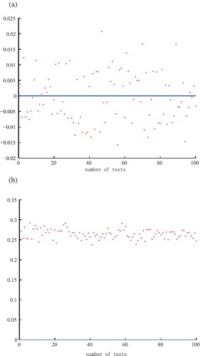
Figure 3. Results of (a) ( – ) and (b) (–), when prediction error is 1.4 and prediction time is .

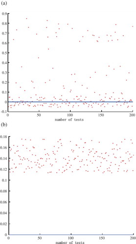
None of the cases below the blue line (x-axis) satisfy Equation (11). The maximum allowable initial errors of the simulated true values are all more than , . In the 100 experiments, is in the range of 0.3224–0.3775 and its average value is 0.3498, while is 24.50% of its average value.

It is clear from Figures 3 and 4 that is not a lower bound estimation of and is a lower bound estimation of . Although is not a lower bound estimation of , it still plays an important role in practical applications. For the reason that for every initial value we can calculate its and then compare it with the accuracy of the analysis value, if we can make sure that the prediction error of the initial value is good, which means the prediction error is less than . It is important to note, however, that the time and space of the calculation will increase because we have to do this for every initial value or observation.

5. Discussion and conclusion

Aimed at the third subproblem of predictability, we analyze the deficiencies of the existing lower bound estimation of the maximum allowable initial error. According to the definition of the maximum allowable initial error, a new lower bound estimation based on the initial observation is presented and proven. The numerical calculation of the new estimation is actualized by using the CNOP method and a PSO algorithm for both the Ikeda and Lorenz96 models. The estimations yielded by the existing and new formulas are compared to demonstrate the shortcomings of the existing estimation.

It is illustrated that is not a lower bound estimation of , but is. Although is not a lower bound estimation of , it still plays an important role in theoretical research and practical applications. It can estimate the range of the maximum allowable initial error, but it is a pity that the calculation time and space will increase because we need to calculate it for every initial state. As for the , the added conditions are stronger during the scaling process, which result in the estimation being much less than the maximum allowable initial error. Combined with the test experiments, we think one reason is that when the prediction time is not so long, the nonlinear effect is not very strong, and the linear effect still plays a big role.

Subsequent work should try to make the estimation more accurate, study its relationship with the maximum allowable initial error in different and nonlinearly stronger models, and obtain the lower bound of the maximum allowable initial error more accurately. Also, considering the high-dimensional characteristics of existing climate models or weather models, it is worth exploring whether a PSO algorithm can perform well in high-dimensional optimization problems.

Figure 4. Results of (a) ( – ) and (b) (–).

Disclosure statement

No potential conflict of interest was reported by the authors.

Additional information

Funding

This work was supported by the National Natural Science Foundation of China (Grant No. 41331174).

References

- Duan, W. S., and H. Y. Luo. 2010. “A New Strategy for Solving A Class of Constrained Nonlinear Optimization Problems Related to Weather and Climate Predictability.” Advances in Atmospheric Sciences 27 (4): 741–749. doi:10.1007/s00376-009-9141-0.
- Ikeda, K. 1979. “Multiple-Valued Stationary State and Its Instability of the Transmitted Light by a Ring Cavity System.” Optics Communications 30: 257–261. doi:10.1016/0030-4018(79)90090-7.
- Kalnay, E. 2002. Atmospheric Modeling, Data Assimilation and Predictability. Cambridge: Cambridge University Press.
- Li, Q., Q. Zheng, and S. Z. Zhou. 2016. “Study on the Dependence of the Two-Dimensional Ikeda Model on the Parameter.” Atmospheric and Oceanic Science Letters 9: 1–6. doi:10.1080/16742834.2015.1128694.
- Lorenz, E. 1996. “Predictability-A Problem Partly Solved.” In Proc. Seminar on Predictability,18 pp. Reading, UK: ECMWF.
- Lorenz, E. N. 1975. “Climate Predictability. The Physical Basis of Climate Modeling.” Global Atmosphere Research Program Publication Series 16:132–136. World Meteorological Organization.
- Mu, M., and W. S. Duan. 2003. “A New Approach to Studying ENSO Predictability: Conditional Nonlinear Optimal Perturbation.” Chinese Science Bulletin 48: 1045–1047. doi:10.1007/BF03184224.
- Mu, M., W. S. Duan, and J. C. Wang. 2002. “The Predictability Problems in Numerical Weather and Climate Prediction.” Advances in Atmospheric Sciences 19: 191–204. doi:10.1007/s00376-002-0016-x.
- Wang, W. Q. 2007. “Research on Ensemble Square Root Filter Assimilation Based on Lorenz - 96 Model.” Master diss., Lanzhou University.
- Yang, Z. B., Q. Zheng, and P. Wang. 2017. “The Applications of the Particle Swarm Optimization to the Predictability Problems.” Journal of PLA University of Science and Technology 2: 135. doi:10.12018/j.issn.1009-3443.20161216001.
- Zheng, Q., Z. B. Yang, J. X. Sha, and J. Yan. 2017. “Conditional Nonlinear Optimal Perturbations Based on the Particle Swarm Optimization and Their Applications to the Predictability Problems.” Nonlinear Processes in Geophysics 24 (1): 1–21. doi:10.5194/npg-24-101-2017.