Role of Atlantic Multidecadal Oscillation (AMO) in winter intraseasonal variability over Ural

ABSTRACT

The modulation of winter intraseasonal variability (ISV) by the Atlantic Multidecadal Oscillation (AMO) is investigated through three sets of reanalysis data and numerical experiments with the NCEP’s atmospheric general circulation model (AGCM). Results show that the positive phase of the AMO tends to intensify ISV activity over the northern Atlantic and shift ISV activity over the Ural Mountains toward the south, causing weakened ISV activity at 200 hPa in the north to the Urals and intensified activity in the south. The modulation of ISV activity by the AMO over the Urals is then explored through comparison of the composite evolution of anomalous ISV cases for the different AMO phases. Fewer ISV cases are found in the AMO positive phase than the negative phase, but no substantial difference in the temporal evolution of anomalous ISV events between the two opposing phases of the AMO. Thus, the AMO exerts its modulation through influencing the occurrence frequency of ISV events, rather than their development or evolution processes. A similar result is seen in the AGCM sensitivity experiments.

Graphical Abstract

摘要

利用多套再分析资料，结合大气环流模式试验，研究了大西洋海温多年代振荡（AMO）对冬季乌拉尔山地区上空大气季节内变率的影响。结果发现：AMO暖位相增强北大西洋上空大气季节内活动，有利于乌拉尔大气季节内变率大值中心向南移动，使得北部大气季节内活动减弱，而南部增强。相比较而言，AMO暖位相期间乌拉尔山上空强大气季节内活动个例明显少于冷位相期间，但不同位相期间季节内活动的发展演变过程并没有明显差异。机制上，AMO通过在北大西洋上空引起热力异常，影响大气准静止波活动，进而调制乌拉尔季节内变率。

KEYWORDS:

• Atlantic Multidecadal Oscillation
• modulation
• intraseasonal variability
• atmospheric stationary wave

关键词:

• 大西洋多年代振荡（AMO）
• 调制
• 大气季节内变率
• 大气静止波

1. Introduction

Intraseasonal variability (ISV) is atmospheric intrinsic variability at time scales beyond the synoptic but smaller than the seasonal, i.e., with a lifespan of 10–90 days. In addition to the well-known ISV over the tropics, like Madden–Julian Oscillation (MJO) (Madden and Julian 1971, 1972), a series of studies have shown the existence of significant ISV in the extratropics and found its important influence on weather and climate on the extended term (e.g., Langley et al. 1981; Rosen and Salstein 1983; Anderson and Rosen 1983; Krishnamurti and Gadgil 1985). A substantial impact of extratropical ISV has been found over East Asia, particularly in winter. For example, Jin and Sun (1996) illustrated the impact of the intraseasonal activity of the East Asian winter monsoon on surface air temperature (SAT) and pressure. Ma, Ding, and Xu (2008) found that a 10–20-day extratropical ISV played an important role in the formation of a strong cold event in winter 2004/05. Wang, Zhang, and Peng (2008) and Ma, Li, and Ju (2011) showed the important roles of both the extratropical ISV and MJO in causing an extreme cold, snowy, and freezing event in January 2008 in southern China. Recently, Ren et al. (2015) documented that the ISV of the Siberian high has a substantial impact on SAT in Southwest China. Thus, understanding the formation of extratropical ISV is of particular meaning for the intraseasonal prediction of the East Asian winter climate, and subsequently for realizing seamless forecasts from the weather to climate scale.

The region around the Ural Mountains (~ 60°N, 60°E) is one of three regions with the strongest ISV activity in mid-to-upper-troposphere geopotential height in the extratropics of the Northern Hemisphere. One important origin of ISV over the Urals is the anomalous persistence or intensified activity of the Urals blocking, which is a key circulation system for the East Asian winter monsoon (Ye et al. 1962). The collapse of the Urals blocking is often the precursor of cold-air outbreaks in East Asia (Tao 1959; Wang et al. 2010). The colder SAT in most regions of central and eastern Asia is closely related with a more frequent occurrence of the Urals blocking (Takaya and Nakamura 2005; Cheung et al. 2013; Wu, Diao, and Zhuang 2016). This is consistent with Yang and Li (2016) analysis based on SAT. The impact of the Urals blocking on the East Asian winter climate can even be seen on the decadal time scale (Wang and Chen 2014; Chang and Lu 2012; Cheung et al. 2015).

The Atlantic Multidecadal Oscillation (AMO) is a basin-scale sea surface temperature (SST) warming or cooling phenomenon in the North Atlantic, with an oscillation periodicity of 65–80 years (Kerr 2000). Previous studies have suggested that the AMO substantially modulates the East Asian summer and winter climate (Lu, Dong, and Ding 2006; Li and Bates 2007; Wang, Li, and Luo 2009; Zhou et al. 2015; Sun, Li, and Zhao 2015; Hong, Lu, and Li 2017). The role of the AMO was also discussed in a recent study by Wang et al. (2017). However, the underlying mechanism for the AMO’s impacts remains poorly understood. Whether the AMO modulates the ISV of the Urals blocking is unclear.

On the one hand, a positive phase of the AMO causes intensified thermal flux from the sea surface of the North Atlantic to the overlying atmosphere and enhanced warmer air advection downstream, which may provide a background favorable for the development and maintenance of atmospheric blocking. On the other hand, it can induce sea-ice reduction in the Barents and Kara seas, which in turn contributes to amplification of the Urals blocking (Luo et al. 2017). Nonetheless, the AMO’s modulation of ISV over the Urals cannot be excluded. Such a consideration motivates the present study, which aims at investigating the modulation of ISV over the Urals by the AMO.

2. Data, methods, and experimental design

2.1. Data and methods

The atmospheric circulation data used in this study include the NCEP–NCAR reanalysis from 1948 to 2015 (Kalnay and Coauthors 1996), the ECMWF’s 20th century reanalysis (ERA-20C) from 1970 to 2015 (Poli et al. 2013), and ERA-Interim from 1979 to 2015 (Dee et al. 2011). The horizontal resolution of these datasets is 2.5° longitude × 2.5° latitude. Winter (November to the following February) daily averaged geopotential heights are utilized. Since the intraseasonal time scale is the focus, Lanczos bandpass filtering is used to extract the components (Duchon 1979) with a time scale of 10–90 days. Before filtering, the climatological annual cycle is removed from the raw data. The climatological annual cycle is calculated as the daily mean during 1970–2010, and a nine-day running mean is then applied to the resultant series to reduce the day-to-day gaps owing to missing data or other mistakes. Due to the limited length of the atmospheric circulation dataset, we use only one AMO positive phase (1996–2015) and one negative phase (1970–90) to reflect the different AMO phases. The SST data used to derive the AMO-related SST anomaly is from the Kaplan Extended SST dataset (version 2), beginning from 1856, which was processed by the Lomont-Doherty Earth Observatory and can be downloaded from NOAA’s Earth System Research Lab website: www.esrl.noaa.gov/~psd.

2.2. Model and experimental design

Sensitivity experiments in an atmospheric general circulation model (AGCM) — an earlier version of the NCEP’s Global Forecasting System for seasonal prediction — are analyzed. The model does not have a well-resolved stratosphere, with the atmospheric top at 10 hPa only, which does not reach the top of the stratosphere (~ 1 hPa). We adapt two sets of experiments performed previously (Li and Bates 2007; Wang, Li, and Luo 2009; Zhou et al. 2015). The first set is termed as the ‘control experiment’, in which the model is forced with the climatological SST seasonal cycle in the North Atlantic (0°–60°N, 75°–7.5°W). The second experiment is termed the ‘AMO+ experiment’, in which the AGCM is forced with the AMO-related SST anomaly added on to the climatological SST. The AMO-related SST anomaly is calculated as the difference of SST in the North Atlantic during the positive-phase AMO period (1935–55) minus that during the negative-phase AMO period (1970–90). So, it is a doubled AMO anomaly. Each experiment consists of three members with an integration period of 12 months starting from initial fields from the NCEP–NCAR reanalysis at 0000 UTC 1–3 September 1980–99, individually. It is equivalent to each member including a total of 20 one-year integrations from September to the following August.

3. Results

3.1. Observational analysis

3.1.1. ISV activity intensity

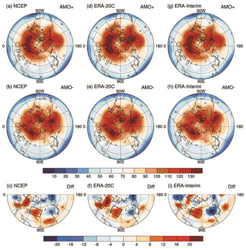
Figure 1 compares the standard deviation of 10–90-day filtered 200-hPa geopotential heights in various datasets for the opposite AMO phases. For the positive phase of the AMO (Figure 1(a,d,g), overall consistency is apparent among the datasets insofar as the three strongest ISV activity centers are over the North Atlantic, North Pacific, and the Ural Mountains. The situation is similar for the negative phase of the AMO (Figure 1(b,e,h)). However, differences between the opposite phases of the AMO are also clear. For example, the activity center over the eastern Atlantic during the positive phase the AMO is evidently stronger than during the negative phase, with the maximum value being 10 m greater (130 m versus 120 m; cf. Figure 1(a,b,d,e,g,h). Besides, the strong ISV activity center over the Urals extends southward during the positive phase of the AMO, with the contour of 100 m closer to Lake Baikal. The difference in ISV activity is seen even more clearly from their difference (Figure 1(c,f,i)). A negative ISV anomaly is located over the northern Urals, along with a positive one in the south. This is seen in all three datasets. Thus, a positive phase of the AMO tends to intensify the ISV over the North Atlantic and shift the ISV activity over the Urals to the south. In other words, the AMO significantly modulates the ISV activity over the Urals.

Figure 1. Comparison of the standard deviation of winter 10–90-day filtered 200-hPa geopotential heights during the different phases of the AMO and their difference. The upper (middle) panels represent the positive-phase (negative-phase) AMO, and the lower panels represent their difference. The left-hand, middle, and right-hand panels correspond to the results derived from NCEP–NCAR, ERA-20C, and ERA-Interim, respectively. The rectangular frames in the lower panels highlight the anomaly region. Dotted areas are statistically significant at the 95% confidence level (F-test). Units: m.

3.1.2. ISV events and their temporal evolution

In this next part of our study we compare the evolution of ISV events during the positive phase of the AMO with that during the negative phase to obtain indications regarding the mechanism for the AMO’s modulation of ISV activity. First, we extract positive or negative ISV events over the Urals from the NCEP–NCAR reanalysis. Then, we conduct a composite analysis for the positive and negative phase the AMO, separately.

Here, a positive (negative) ISV event is defined as when the filtered 200-hPa geopotential height anomaly over the Urals (60°E, 60°N) is greater than 1.5 (smaller than −1.5) times the standard deviation. As such, a total of 55 cases (26 positive and 29 negative) are obtained for the positive-phase AMO period. Meanwhile, a total of 74 cases (31 positive events and 43 negative) are derived for the negative-phase AMO. There are evidently fewer cases in the positive phase the AMO relative to the negative phase (55 versus 74). This is in agreement with the southward shift of the Urals ISV activity, as seen in the lower panels of Figure 1 (negative anomalies of standard deviation over the Urals).

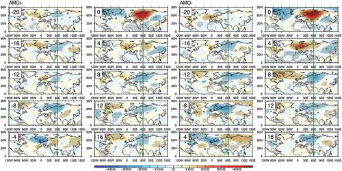
Since a power spectral analysis of daily 200-hPa geopotential heights over the Urals suggests a peak periodicity of 10–40 days for both the positive- and negative-phase AMO (not shown), a composite evolution of a total of 40 days, 20 days prior to the ISV occurrence and 20 days since its disappearance, is analyzed. Figure 2 compares the composite evolution of ISV events derived from the positive-phase AMO with that from the negative phase. Because of an overall symmetry, the difference of the positive ISV cases minus the negative cases is shown here. For the composite from the cases in the positive AMO phase period (the two left columns in Figure 2), on day(−16), a negative height anomaly is located over the Urals. Then, it moves westward and develops, reaching the northeastern Atlantic and West Europe on day(−4). Meanwhile, a positive height anomaly develops over Siberia, then propagates westward and reaches the Urals. The positive height anomaly develops rapidly and reaches its maximum on day(0). It then weakens and breaks into two centers before vanishing on day(8). At the same time, a negative anomaly develops rapidly over the Urals. For the ISV events derived from the cases in the negative-phase AMO (the two right columns in Figure 2), the composite evolution exhibits a similar process, albeit with a discernible difference in magnitude. For example, the maximum anomaly in the positive-phase AMO is visually smaller than that in the negative-phase AMO, which is even clearer on day(0) and day(4). This suggests that the AMO’s phase does not influence the development and evolution, but does influence the occurrence and amplitude, of the ISV over the Urals.

Figure 2. Comparison of the composite evolution of 10–40-day filtered 200-hPa geopotential heights during the positive AMO phase with those during the negative AMO phase. Displayed is the difference of the positive ISV cases minus the negative ISV cases from day(−20) to day(16), with an interval of 4 days. Units: m. Dotted areas are statistically significant at the 95% confidence level (Student’s t-test).

3.2. AGCM results

3.2.1. ISV activity intensity

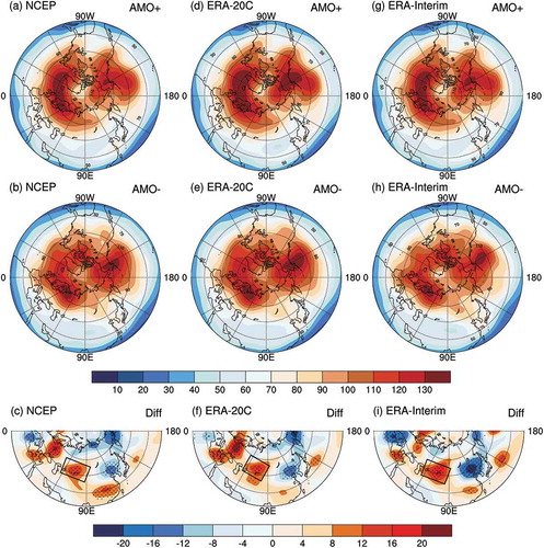
Figure 3 displays the standard deviation of filtered 200-hPa geopotential heights in the AGCM experiments. In comparison with the observational results (cf. Figures 1 and 3), the simulated ISV activity centers show consistency, with the maxima over the North Pacific and North Atlantic, extending eastward to reach western Siberia, albeit the latter being relatively weaker. This suggests that the model captures the observed ISV activity well, forming a basis for elucidating the AMO’s influence on ISV by using the AGCM experiments.

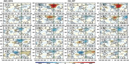
Figure 3. Comparison of standard deviation of winter 10–90-day filtered 200-hPa geopotential heights in different sets of AGCM experiments. (a) is from the ‘AMO+ SSTA’ experiment; (b) is from the control experiment; (c) is the difference of (a) minus (b).

Comparing the results from ‘AMO+ Experiment’ with ‘Control Experiment’, the simulated climatological ISV activity over the Urals in the former is obviously weaker, along with intensified ISV activity in the south of the Urals. In other words, the simulated ISV in the SST-forced experiments shifts evidently to the south. This shift is even clearer in their difference plot (Figure 3(c)), with positive values in the southern Urals but negative values in the north. Besides, the simulated ISV activity over the North Atlantic (55°–60°N, 0°–30°E) in the AMO-SST-forced experiments is evidently weaker than in the control experiment. These results bear an overall consistency with the observational findings (cf. Figure 1(c,f,i) with Figure 3(c)).

3.2.2. ISV events over the Urals and their temporal evolution

As in the observational analysis, we compare the ISV events over the Urals in the AMO-SST-forced experiments with those in the control experiments. Based on the same method, a total of 72 ISV events (32 positive and 40 negative) are derived from the SST-forced experiment. The number of ISV events is 74 in the control experiments, consisting of half positive and half negative. Regardless of the polarity of ISV events, there are fewer ISV cases corresponding to the positive-phase AMO (72 versus 74). This illustrates that a positive AMO favors a weakening of ISV events over the Urals, as seen in the observational analysis.

Figure 4 compares the composite temporal evolution of ISV events derived from the AMO-SST-forced and control experiments. As in the observational analysis (Figure 2), we compare the difference in positive ISV cases minus negative cases. From the results, the development and evolution processes in the AGCM experiments are similar to those seen in the observational analysis, in that no significant difference is seen between the two experiments. This suggests that the AMO exerts its modulation through affecting the occurrence rather than the development and evolution of ISV events over the Urals, consistent with the observational findings. No significant modulation by the AMO of the development and evolution of ISV events over the Urals seems reasonable, since the SST forcing does not usually change the intrinsic atmospheric dynamics (e.g., Peng and Robinson 2001).

Figure 4. Composite evolution of 10–40-day filtered 200-hPa geopotential heights of the ISV cases in the AGCM experiments. Displayed is the difference of the positive ISV cases minus the negative ISV cases. The left two columns are for the ‘AMO+ SST’ experiments, and the right two columns are for the control experiments.

4. Concluding remarks and discussion

The AMO’s modulation of ISV activity over the Urals is studied through three sets of reanalysis data and AGCM sensitivity experiments, and the results provide form evidence for such a relationship. Specifically, a positive phase of the AMO tends to intensify the ISV activity over the North Atlantic and shift the ISV activity to the south. However, the AMO does not change the development and evolution processes of the Urals ISV. Consistency is found between the observational results and those of the AMO-SSTA-forced experiments. Thus, the AMO’s modulation of the ISV over the Urals is robust.

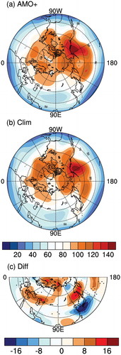
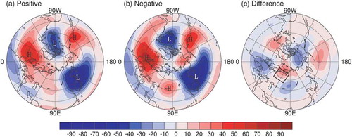
Why the AMO modulates the occurrence of Urals ISV events remains unclear. It is well known that atmospheric stationary waves play a role in the maintenance and variation of ISV. Figure 5 compares the observed atmospheric stationary wave activity, expressed as the winter seasonal mean 500-hPa geopotential height with the zonal-mean removed, in the different AMO phases. Clearly, there is a wavenumber-three stationary structure in the mid-to-high latitudes, regardless of the polarity of the AMO, with deep troughs over East Asia and North America, respectively, along with one shallow trough over Europe. However, a substantial difference exists between the different AMO phases (cf. Figure 5(a,b)) insofar as, during the AMO positive phase, the stationary ridge over the eastern North Atlantic is significantly weaker, and meanwhile the ridge over the Urals is obviously stronger and shifts to the north. This is even clearer in their difference plot (Figure 5(c)), with a negative anomaly over the eastern North Atlantic and a positive one over the Urals. This implies that the difference in stationary waves between the opposite AMO phases may play a role in modulating the ISV activity. The observed weakened stationary ridge over the eastern North Atlantic can be explained by the AMO-related warm SST, which can be seen from the simulated negative height response to the AMO in Wang, Li, and Luo (2009, Figure 12, left-hand panels).

Figure 5. Comparison of stationary waves at the winter geopotential height of 500 hPa during the different phases of the AMO: (a, b) positive- and negative-phase AMO; (c) their difference. ‘H’ indicates the stationary ridge; ‘L’ indicates the stationary trough. The frame in (c) represents the location of the climatological ridge around the Urals. Units: m.

In addition, stratosphere–troposphere coupling may play a role in connecting the AMO with the ISV over the Urals (Omrani et al. 2014). The AMO-related downward propagating signal from the stratosphere might contribute to the ISV. Thus, the AGCM without a well-resolved stratosphere will be unable to simulate the downward propagating signal, resulting in weaker ISV responses. The evidently weaker standard deviation and responses in the AGCM (cf. Figures 3 and 4 with Figures 1 and 2) may be attributable in part to the poor expression of the stratosphere in the AGCM used here, which has an atmospheric top at 10 hPa.

Recently, Li et al. (forthcoming) demonstrated that the cold phase of the AMO tends to be associated with a more frequent occurrence of the Urals blocking, which to a certain extent backs up our findings. Besides, Luo et al. (2017) revealed increased quasi-stationarity and persistence of the Urals blocking in the context of Arctic warming. Considering that the ISV over the Urals is in part related to the long persistence of the blocking, and the recent rapid warming of the Arctic coincides with a shift in the AMO phase from negative to positive, an outstanding issue is the relative importance of Arctic warming and the AMO in determining the nature of the Urals ISV. This issue is deserving of further study.

Finally, it is important to acknowledge that the period used to derive the positive-AMO-related SSTA (1935–55) for the experiments does not match that used to derive the atmospheric circulation variability (1996–2015). This is certainly a caveat of the present study; however, a qualitative resemblance between the AMO-related SSTA in the two periods can be found (not shown). Furthermore, in the observational analysis we only compare one AMO positive-phase period (1996–2015) and one negative-phase period (1970–1990) to derive the AMO’s modulation of the ISV. This too is recognized as a limitation that should be addressed in follow-up work.

Disclosure statement

No potential conflict of interest was reported by the authors.

Additional information

Funding

This work was jointly supported by the Strategic Priority Research Program of the Chinese Academy of Sciences [grant number XDA19070401], the National Natural Science Foundation of China [grant numbers 41790473 and 41421004], and the Fundamental Research Funds for the Central Universities.

References

- Anderson, J. R., and R. D. Rosen. 1983. “The Latitude-Height Structure of 40–50 Day Variation in Atmospheric Angular Momentum.” Journal of the Atmospheric Sciences 40 (6): 1584–1591. doi:10.1175/1520-0469(1983)040<1584:TLHSOD>2.0.CO;2.
- Chang, C.-P., and -M.-M. Lu. 2012. “Intraseasonal Predictability of Siberian High and East Asian Winter Monsoon and Its Interdecadal Variability.” Journal of Climate 25: 1773–1778. doi:10.1175/JCLI-D-11-00500.1.
- Cheung, H. H. N., W. Zhou, S. Lee, and H. Tong. 2015. “Interannual and Interdecadal Variability of the Number of Cold Days in Hong Kong and Their Relationship with Large-Scale Circulation.” Monthly Weather Review 143: 1438–1454. doi:10.1175/MWR-D-14-00335.1.
- Cheung, H. N., W. Zhou, Y. Shao, W. Chen, H. Y. Mok, and M. C. Wu. 2013. “Observational Climatology and Characteristics of Wintertime Atmospheric Blocking over Ural-Siberia.” Climate Dynamics 41: 63–79. doi:10.1007/s00382-012-1587-6.
- Dee, D. P., S. M. Uppala, A. J. Simmons, P. Berrisford, P. Poli, S. Kobayashi, U. Andrae, et al. 2011. “The ERA-Interim Reanalysis: Configuration and Performance of the Data Assimilation System.” Quarterly Journal of the Royal Meteorological Society 137 (656): 553–597. DOI:10.1002/qj.828.
- Duchon, C. E. 1979. “Lanczos Filtering in One and Two Dimensions.” Journal of Applied Meteorology 18 (8): 1016–1022. doi:10.1175/1520-0450(1979)018<1016:LFIOAT>2.0.CO;2.
- Hong, X., R. Lu, and S. Li. 2017. “Amplified Summer Warming in Europe-West Asia and Northeast Asia after the Mid-1990s.” Environmental Research Letters 12 (9): 094007. doi:10.1088/1748-9326/aa7909.
- Jin, Z. H., and S. Q. Sun. 1996. “The Characteristics of Low Frequency Oscillations in Winter Monsoon over the Eastern Asia.” Scientia Atmospherica Sinica 20 (1): 101–111. [in Chinese.].
- Kalnay, E.,M. Kanamitsu, R. Kistler, W. Collins, D. Deaven, L. Gandin, M. Iredell, et al. 1996. “The NCEP/NCAR 40-Year Reanalysis Project.” Bulletin of the American Meteorological Society 77 (3): 437–471. doi:10.1175/1520-0477(1996)077<0437:TNYRP>2.0.CO;2.
- Kerr, R. A. 2000. “A North Atlantic Climate Pacemaker for the Centuries.” Science 288 (5473): 1984–1985. doi:10.1126/science.288.5473.1984.
- Krishnamurti, T. N., and S. Gadgil. 1985. “On the Structure of the 30 to 50day Mode over the Globe during FGGE.” Tellus 37A: 336–360. doi:10.1111/j.1600-0870.1985.tb00432.x.
- Langley, R. B., R. W. King, I. I. Shapiro, R. D. Rosen, and D. A. Salstein. 1981. “Atmospheric Angular Momentum and the Length of Day: A Common Fluctuation with A Period near 50 Days.” Nature 294 (5843): 730–732. doi:10.1038/294730a0.
- Li, F., Y. J. Orsolini, H. Wang, Y. Gao, and S. He. forthcoming. “Atlantic Multidecadal Oscillation Modulates the Impacts of Arctic Sea Ice Decline.” Geophy Researcher Letters. doi:10.1002/2017GL076210.
- Li, S., and G. T. Bates. 2007. “Influence of the Atlantic Multidecadal Oscillation on the Winter Climate of East China.” Advances in Atmospheric Sciences 24 (1): 126–135. doi:10.1007/s00376-007-0126-6.
- Lu, R., B. Dong, and H. Ding. 2006. “Impact of the Atlantic Multidecadal Oscillation on the Asian Summer Monsoon.” Geophysical Research Letters 33 (24): 194–199. doi:10.1029/2006GL027655.
- Luo, D., Y. Yao, A. Dai, and I. Simmonds. 2017. “Increased Quasi-Stationarity and Persistence of Ural Blocking in Response to Arctic Warming. Part II: A Theoretical Explanation.” Journal of Climate 30 (10): 3569–3587. doi:10.1175/JCLI-D-16-0262.1.
- Ma, N., Y. F. Li, and J. H. Ju. 2011. “Intraseasonal Oscillation Characteristics of Extreme Cold, Snowy and Freezing Rainy Weather in Southern China in Early 2008.” Plateau Meteorology 30 (2): 318–327. [In Chinese].
- Ma, X. Q., Y. H. Ding, and H. M. Xu. 2008. “The Relation between Strong Cold Waves and Low-Frequency Waves during the Winter of 2004/2005.” Chinese Journal of Atmospheric Sciences 32 (2): 380–394. [In Chinese].
- Madden, R. A., and P. R. Julian. 1971. “Detection of a 40–50 Day Oscillation in the Zonal Wind in the Tropical Pacific.” Journal of Atmospheric Sciences 28 (5): 702–708. doi:10.1175/1520-0469(1971)028<0702:DOADOI>2.0.CO;2.
- Madden, R. A., and P. R. Julian. 1972. “Description of Global-Scale Circulation Cells in the Tropics with a 40–50 Day Period.” Journal of Atmospheric Sciences 29: 1109–1123. doi:10.1175/1520-0469(1972)029<1109:DOGSCC>2.0.CO;2.
- Omrani, N.-E., N. S. Keenlyside, J. Bader, and E. Manzini. 2014. “Stratosphere Key for Wintertime Atmospheric Response to Warm Atlantic Decadal Conditions.” Climate Dynamics 42: 649–663. doi:10.1007/s00382-013-1860-3.
- Peng, S., and W. A. Robinson. 2001. “Relationships between Atmospheric Internal Variability and the Responses to an Extratropical SST Anomaly.” Journal of Climate 14 (13): 2943–2959. doi:10.1175/1520-0442(2001)014<2943:RBAIVA>2.0.CO;2.
- Poli, P., H. Hersbach, D. G. H. Tan, D. P. Dee, J.-N. Thépaut, A. Simmons, C. Peubey, et al. 2013. “The Data Assimilation System and Initial Performance Evaluation of the ECMWF Pilot Reanalysis of the 20th-Century Assimilating Surface Observations Only (ERA-20C).” ERA Report 14: 59.
- Ren, J. Z., J. M. Zheng, Y. Y. Xu, Y. Tao, W. C. Zhang, and J. H. Ju. 2015. “The Interseasonal Oscillation of Siberian High Influenced on the Winter Temperature of Yunnan in 2007.” Journal of Yunnan University 37 (3): 386–398. [in Chinese.].
- Rosen, R. D., and D. A. Salstein. 1983. “Variations in Atmospheric Angular Momentum on Global and Regional Scales and the Length of Day.” Journal of Geophysical Research Atmospheres 88 (C9): 5451–5470. doi:10.1029/JC088iC09p05451.
- Sun, C., J. Li, and S. Zhao. 2015. “Remote Influence of Atlantic Multidecadal Variability on Siberian Warm Season Precipitation.” Sciences Reports 5: 16853. doi:10.1038/srep16853.
- Takaya, K., and H. Nakamura. 2005. “Mechanisms of Intraseasonal Amplification of the Cold Siberian High.” Journal of Atmospheric Sciences 62: 4423–4440. doi:10.1175/JAS3629.1.
- Tao, S. Y. 1959. ““Study on East Asian Cold Waves in China during Recent 10 Years (1949–1959).”[In Chinese.].” Acta Meteorologica Sinica 30 (3): 226–230. doi:10.11676/qxxb1959.031.
- Wang, L., and W. Chen. 2014. “The East Asian Winter Monsoon: Re-Amplification in the Mid-2000s.” Science Bulletin 59 (4): 430–436. doi:10.1007/s11434-013-0029-0.
- Wang, L., W. Chen, W. Zhou, J. C. L. Chan, D. Barriopedro, and R. Huang. 2010. “Effect of the Climate Shift around Mid 1970s on the Relationship between Wintertime Ural Blocking Circulation and East Asian Climate.” International Journal of Climatology 30: 153–158.
- Wang, L., P. Xu, W. Chen, and Y. Liu. 2017. “Interdecadal Variations of the Silk Road Pattern.” Journal of Climate 30: 9915–9932. doi:10.1175/JCLI-D-17-0340.1.
- Wang, Y., S. Li, and D. Luo. 2009. “Seasonal Response of Asian Monsoonal Climate to the Atlantic Multidecadal Oscillation.” Journal of Geophysical Research Atmospheres 114 (D2): 356–360.
- Wang, Y., Q. Y. Zhang, and J. B. Peng. 2008. “Relationship between the Intraseasonal Oscillation of East Asian Monsoon Circulation and the Heavy Snow over Southern China in Boreal Winter of 2007/2008.” Climatic and Environmental Research 13 (4): 459–467. [in Chinese.].
- Wu, J., Y. N. Diao, and X. Z. Zhuang. 2016. “The Relationship between the Ural Blocking in Boreal Winter and the East Asian Winter Monsoon.” Climatic and Environmental Research 21 (5): 577−585. [in Chinese.].
- Yang, S., and T. Li. 2016. “Intraseasonal Variability of Air Temperature over the Mid-High Latitude Eurasia in Boreal Winter.” Climate Dynamics 47: 2155–2175. doi:10.1007/s00382-015-2956-8.
- Ye, D. Z., S. Y. Tao, B. Zhu, J. Yang, and L. Chen. 1962. The Study on Wintertime Blocking Pattern of the Northern Hemisphere. Beijing: Chinese Science Press. 220. [in Chinese.].
- Zhou, X. M., S. Li, F. F. Luo, Y. Gao, and T. Furevik. 2015. “Air–Sea Coupling Enhances the East Asian Winter Climate Response to the Atlantic Multidecadal Oscillation.” Advances in Atmospheric Sciences 32 (12): 1647–1659. doi:10.1007/s00376-015-5030-x.