Improved EOF-based bias correction method for seasonal forecasts and its application in IAP AGCM4.1

ABSTRACT

An effective improvement on the empirical orthogonal function (EOF)–based bias correction method for seasonal forecasts is proposed in this paper, by introducing a stepwise regression method into the process of EOF time series correction. Using 30-year (1981–2010) hindcast results from IAP AGCM4.1 (the latest version of this model), the improved method is validated for the prediction of summer (June–July–August) rainfall anomalies in Southeast China. The results in terms of the pattern correction coefficient (PCC) of rainfall anomalies shows that the 30-year-averaged prediction skill improves from 0.01 to 0.06 with the original correction method, and to 0.29 using the improved method. The applicability in real-time prediction is also investigated, using 2016 summer rainfall prediction as a test case. With a PCC of 0.59, the authors find that the new correction method significantly improves the prediction skill; the PCC using the direct prediction of the model is −0.04, and using the old bias correction method it is 0.37.

Graphical Abstract

摘要

本文针对短期气候预测中的EOF误差订正方法，提出基于逐步回归改进EOF订正模态的选取及确定各模态对应时间系数的方法。改进后的订正方法显著提高了IAP AGCM4.1对中国东南地区夏季降水异常的预测技巧，30年（1981–2010年）平均的观测与订正后的模式回报夏季降水距平的空间相关系数（PCC）达到0.29，远高于订正前的0.01。该方法应用于2016年夏季降水的实际预测检验表明，采用改进后的订正方法可使得预测与模式预测结果的PCC提高到0.59，显著优于采用了改进前的订正方法的结果（PCC = 0.37）。

KEYWORDS:

• Bias correction
• seasonal forecast
• prediction skill
• IAP AGCM4.1

关键词:

• 误差订正；季节预测；预报技巧；IAP AGCM4.1大气环流模式

1. Introduction

Given the considerable socioeconomic damage that can be cause by major meteorological disasters, improving the accuracy of seasonal climate prediction is a long-standing challenge in climate research (Zeng 2009; Wang et al. 2015; MacLachlan et al. 2015). Indeed, existing climate prediction systems suffer from many shortcomings, such as imperfect model physics or initial conditions. Therefore, a large variety of post-treatment techniques, including bias correction methods, have been proposed and developed by many investigators (e.g. Christensen et al. 2008; Li, Sheffield, and Wood 2010), and have also been applied in real-time prediction (e.g. Lin et al. 1998; Chen and Lin 2006). Among them, a bias correction method based on the empirical orthogonal function (EOF) was proposed by Zeng et al. (1994). It considers the spatial correlation between observation and prediction, and has been widely used in seasonal prediction (Yun et al. 2005; Li et al. 2005).

Based on the second generation IAP dynamical extra-seasonal climate prediction system (IAP DCP-II) (Lin et al. 1998; Zeng, Lin, and Zhou 2003), Qin et al. (2011) developed an EOF-based bias correction method (hereinafter referred to as ‘QLS’) as a new component of IAP DCP-II to remove the model systematic bias, and significant improvement was found in the seasonal summer rainfall prediction skill over China. However, when considering each individual year, the bias-corrected results exhibited no significant improvement, and even became worse in 4 of the 20 hindcast years. This suggests that there is still room for further improvement to the QLS method used in IAP DCP-II.

Recently, a new version of the IAP’s AGCM (namely, IAP AGCM4.1) has been released, and its performance in reproducing the observed climatology has been evaluated (e.g. Lin et al. 2016; Wang et al. 2016). To update the dynamical seasonal prediction system within IAP AGCM4.1, the efficiency and applicability of the QLS method in IAP AGCM4.1 needs to be assessed. In this paper, using 30-year hindcast results from IAP AGCM4.1, we investigate the efficiency of the QLS method in terms of the prediction skill of summer rainfall over Southeast China. The deficiencies of the method are then further analyzed, and an improved EOF-based bias correction method is proposed. Finally, the effectiveness of the improved method in terms of the seasonal prediction skill is demonstrated through its application in the hindcast experiment and real-time prediction of summer rainfall anomalies over Southeast China.

2. Hindcast experiment and data

The model used in this study is IAP AGCM4.1, which is the latest version of the IAP’s AGCM, with a horizontal resolution of 1.4° × 1.4° and 30 levels in the vertical direction (Zhang, Lin, and Zeng 2009). Hindcast experiments for a 30-year period (1981–2010) are conducted, wherein the experiment in each year is initiated from 0000 UTC 1 March to 1800 UTC 5 March with atmospheric initial conditions taken from NCEP’s CFSR (Saha et al. 2010) at intervals of 6 h and a forecast lead time of up to six months. Thus, there are 30 years of hindcasts with a 20-member ensemble for each individual year, and all the ensemble members are treated equally to calculate the ensemble mean for each year. The SST anomaly (SSTA) used in the ensemble hindcast is a weighted summation according to the observed February SSTA from Hadley/OI SST and the forecasted SSTA of the IAP’s ENSO ensemble prediction system (Zheng et al. 2006).

The observed monthly rainfall data used in this study are from the CN05.1 gridded dataset, originally developed by Wu and Gao (2013), which have a horizontal resolution of 1° × 1° and cover the period 1961–2017. The IAP AGCM4.1 hindcast data are bilinearly interpolated from 1.4° × 1.4° to 1° × 1° for analysis.

3. Results

3.1. Prediction skill of summer rainfall anomalies over southeast china in IAP AGCM4.1

The prediction skill of IAP AGCM4.1 summer rainfall in Southeast China is demonstrated using the temporal correlation coefficient (TCC) between observed and hindcast rainfall anomalies during 1981–2010, as shown in Figure 1(a). Relatively higher TCCs can be seen between the Yangtze and Yellow river basins, with a maximum TCC of more than 0.2. However, the prediction skill of summer rainfall anomalies in Southeast China is low, with TCCs lower than −0.2 over most parts of South China, and the lowest value being approximately −0.4 near the middle reaches of the Yangtze River.

Figure 1. (a) TCCs between the observed and hindcast summer rainfall anomaly in Southeast China during the 30 years from 1981–2010. (b) TCCs between the observation- and the QLS-based result during the 30 years from 1981–2010. (c) Observed total summer precipitation in 1998. (d–f) Summer rainfall anomaly percentage in 1998 based on observation, hindcast, and the QLS method.

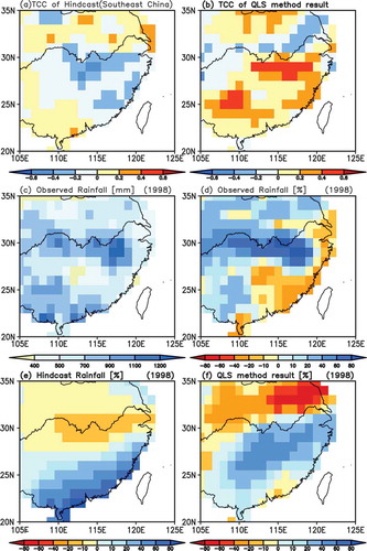
Figure 1(b) shows the TCCs between observed and hindcast summer rainfall anomalies after bias correction using the QLS EOF-based method. After QLS bias correction, the TCCs over the south of the Yangtze River increase significantly, with values exceeding 0.4 over most parts of Southeast China. However, along the lower reaches of the Yangtze River the TCCs change to negative values lower than −0.2, where they are positive in the uncorrected results. However, we find that the 30-year mean pattern correlation coefficient (PCC) increases from 0.01 to 0.06. These results suggest that the QLS method can generally improve the summer rainfall prediction skill over most parts of Southeast China, but the prediction skill can also become worse in certain regions after correction.

The effectiveness of the QLS method is further assessed for the prediction of rainfall in a specific year, i.e. 1998, when severe flooding occurred across the whole of China, especially in the south. Figure 1(c) shows the summer rainfall distribution over Southeast China. The summer precipitation amount is more than 700 mm from the Yangtze River to the west part of South China, and the precipitation over the middle reaches of the Yangtze River reaches 1300 mm. Figure 1(d) is the distribution of percentage summer rainfall anomalies, with 1981–2010 as the base period. Significant positive percentage anomalies can be found over Southeast China, with maximum percentage anomalies larger than 80% near the middle reaches of the Yangtze River. Unfortunately, the hindcast result feature large bias; anomalies along the Yangtze River are negative (−20% to −10%), while the positive rainfall anomaly values are mainly distributed over the south of the Yangtze River, with the anomaly percentage reaching 60% near the coast (Figure 1(e)).

Treating 1998 as the prediction year, the hindcast and observational data from 1981 to 2010 (except 1998) are used for correction. We can see from Figure 1(f) that the bias-corrected pattern of rainfall anomalies is improved over the Yangtze river basin, with the PCC between the observed and predicted results over Southeast China increasing from −0.45 to 0.07. The rainy areas over the middle and lower reaches of the Yangtze River are reproduced, with positive rainfall anomalies ranging from 20% to 40%. However, even after QLS bias correction, the predicted rainfall anomalies along the upper reaches of the Yangtze River and the Huaihe River Basin are still negative, which is inconsistent with observation. This suggests that the prediction skill is generally improved by the QLS method, but limitations still exist.

3.2. Improvement of the EOF-based bias correction method

As described in Qin et al. (2011), the EOF bias correction method is based on the spatial patterns and time series (i.e. principal component (PC)) of the observations and hindcasts by the EOF. Firstly, the regression relationships are established between the PCs of the observations and hindcasts; then, those PCs of the corrected prediction are modified according to the relationships, and the observed EOF spatial pattern is used to replace the EOF pattern of the hindcast. Finally, the corrected prediction result is obtained by the product of the modified PCs and the observed EOF spatial patterns.

As the first five EOF modes of the 30-year CN05.1 rainfall data in Southeast China carry 73.03% of the total variance, the QLS bias correction applied as above is based on these five dominant modes. Figure 2 shows the patterns of the five dominant modes based on observation and the hindcast results of IAP AGCM4.1 during 1981–2010. We can see that IAP AGCM4.1 is basically able to capture the dominant patterns of rainfall in Southeast China.

Figure 2. EOF pattern of the five dominant modes of 30-year observation and hindcast. The percentage value in each panel is the explained variance. The PCC between observation and hindcast EOF Modes 1–5 are 0.87, 0.61, 0.60, 0.42, and 0.24, respectively.

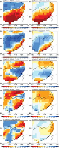
The pattern of observed EOF Mode 1 shows the opposite rainfall anomalies north and south of the Yangtze River. The EOF Mode 1 of the model hindcast captures these characteristics well, with the PCC of EOF Mode 1 between observation and hindcast reaching 0.87. The observed EOF Mode 2 shows positive rainfall anomalies along the Yangtze River and in the western part of South China, and negative anomalies over the northern part of the Huaihe River basin and South China coast. The hindcast Mode 2 reproduces the main pattern, with the PCC between them of 0.61. The observed EOF Mode 3 shows a negative–positive–negative tripolar pattern, with the anomaly in the eastern part of South China being opposite to the other areas; and the hindcast Mode 3 has similar features, with a PCC of 0.60. The observed pattern of Mode 4 shows positive anomalies along the lower reaches of the Yangtze River and the middle part of South China, and significant negative anomalies over the Huaihe River basin and other regions of South China. The hindcast EOF Mode 4 basically captures the anomaly characteristics over the Huaihe River basin and South China, except for the positive anomalies over the Yangtze River. The PCC between them is 0.42, which is relatively low compared with the first three modes. There are clear differences between the observed and hindcast EOF Mode 5. The observed Mode 5 shows positive anomalies over the western part of the Huaihe River basin, the area near the lower reaches of the Yangtze River, and in the middle part of South China; while negative anomalies occupy the Yangtze River delta, the western part of South China, and over the eastern South China coast. The hindcast Mode 5, however, can only simulate the positive anomalies in the Huaihe River Basin; the anomaly characteristics in other regions are almost completely opposite to observation.

The correlation coefficient between the time series of observed and hindcast PCs of Mode 1 is 0.04, for both mode 2 and mode 3 it is −0.29, for mode 4 it is −0.03, and for mode 5 it is 0.57. These results suggest that IAP AGCM4.1 cannot reproduce the observed temporal variation of the first four EOF patterns, even though the spatial patterns of these four dominant EOF modes agree well with observation. Therefore, EOF-based bias correction should be accomplished through modifying the PCs of each mode.

We next check the possible reasons for the failure of the QLS method in improving the summer rainfall anomalies in 1998. As summarized in Table 1, we find that the observed summer rainfall pattern for 1998 is dominated by Mode 2, Mode 4, and Mode 5, as shown in Figure 2. PC2, PC4, and PC5 from observation are equal to 1.74, −0.73, and 1.28 respectively, so the observed rainfall pattern is mainly a combination of positive Mode 2 and Mode 5, and negative Mode 4. They provide the main features of the 1998 summer rainfall anomalies (Figure 1(d)), i.e. the positive anomaly in the Huaihe River Basin, along the Yangtze River, and in southwest China; and negative anomalies in the area around the Yangtze River delta and the southeast coast.

Table 1. PCs of the five dominant modes in 1998.

	Observation	Hindcast	QLS correction	Improved correction
Mode1	0.1327	−2.5660	−1.0368	0.1380
Mode2	1.7377	−1.6346	0.5799	1.5009
Mode3	0.1407	−0.5991	1.9662	1.2760
Mode4	−0.7276	1.0428	1.2351	0.9991
Mode5	1.2822	0.7674	−0.2971	0.8900

As shown in Table 1, different from observation, Mode 1 is the most significant for the IAP AGCM4.1 hindcast result, with a PC1 value of −2.57. We also find that the signs of the PCs of the four dominant hindcast modes are all opposite to observation, except Mode 5. Moreover, the overly large weight of Mode 1 leads to the positive anomalies being mainly located over South China in the hindcast result, while the opposite signs of modes cause the rainfall pattern in most areas to be opposite to that observed (Figure 1(e)). Therefore, the key issue for the QLS EOF-based bias correction method is whether the PCs for each dominant mode can be modified efficiently close to observation.

Following the original method proposed by QLS, modified PCs are also shown in Table 1. As the hindcast EOF pattern will be replaced with the observed one after correction, here, we only evaluate the correction effect on the model hindcast PCs. The improvements observed in the corrected result are that the signs of Mode 2 and Mode 3 become the same as observed, and the weight of Mode 1 decreases. However, the signs of Mode 1, Mode 4, and Mode 5 are still incorrect, and obvious bias still exists in each mode’s weight. Negative Mode 1 incorrectly contributes the positive anomaly in South China. The lower weight of Mode 2 leads to the percentage rainfall anomalies ranging from 20% to 40% along the Yangtze River — far less than the observed value of 80%. The region with a false negative anomaly in the Huaihe River Basin is attributed to the excessively positive Mode 3 and Mode 4 (Figure 1(f)).

To explain the reason for the poor correction of PCs, the regression effect of the multiple linear regression method used in the bias correction is tested. Following the QLS method, the first k PCs of the hindcast are used in regression with each PC of the observation. The multiple linear regression equation can be expressed as

(1)

where is the PCs of observation, is the PCs of the hindcast, is the regression coefficient, is the regression deviation, i is the mode number of the hindcast, and j is the mode number of observation. Here, we set the value of k as 10.

The regression equation of the first observed mode in 1998 is as follows:

(2)

The F-test, which can calculate the joint significance of a group of variables, is used. The F-value in the regression is the result of a test in which the null hypothesis is that all of the regression coefficients are equal to zero. The F-value of regression Equation (2) is 0.3129, which means that the significance of this equation is only approximately 68.71%. The regression relationship between the observed and hindcast PCs is unstable, which will lead to a limited correction effect for prediction.

Stepwise regression is considered a better regression method for this problem, because the independent variables that have a weak regression relationship with the dependent variable will be eliminated. Using stepwise regression, the regression equation with the best significance is combined with three hindcast modes:

(3)

The F-value of the new equation is 0.0095, which means that it can pass the 0.01 significance test. The regression relationship is much more stable. Here, we define the number of hindcast modes used for regression as n. The regression equations of other observed PCs have similar results, and the n value for all of the observed modes is three. Then, the new PCs of the first five modes in 1998 are calculated (see Table 1). Compared with the corrected results with the original QLS method, the values of PC1, PC3, and PC5 are much closer to the observed values, and the signs of the PCs are the same as those of the observations, except for Mode 4.

Although the effectiveness of the new regression method has been demonstrated for 1998, its suitability for other years needs to be further tested. Figure 3(a) shows the correlation coefficients between the 30-year time series of the observed and corrected hindcast PCs for each mode, which shows the prediction skill of the corrected PCs. The correlation coefficient values change with the number of hindcast modes used in the regression for each observed mode. The hindcast mode with the best regression relationship with observed mode is used firstly, then the second-best hindcast mode, until the worst hindcast mode of the first 10 modes is added in the regression.

Figure 3. (a) Correlation coefficient between the 30-year time series of observed PCs and the corrected hindcast PCs. The values change with the number of hindcast modes used in the regression. (b) The 30-year average of the PCC between the observed and corrected rainfall anomaly in Southeast China based on the two correction methods. The values change with the hindcast modes used in the correction methods. (c–f) Order numbers of the hindcast mode with the best three regression relationships with the time series of observed PCs over 30 years.

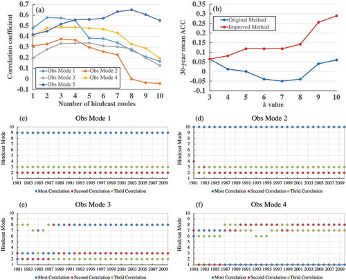
Here, we take observed Mode 2 as an example. When the hindcast mode with the best regression relationship is used to establish the regression equation (n = 1), the correlation coefficient between the 30-year observed PC2 and corrected PCs is 0.31. As the second-best hindcast modes are added (n = 2), the correlation coefficient increases to 0.33. When the best three hindcast modes are used (n = 3), the value of the correlation coefficient reaches a peak at 0.38. After the fourth best hindcast mode is added (n = 4), the correlation coefficient decreases to 0.37, and the value becomes lower as more modes are added. When all 10 modes have been added (n = 10), the correlation coefficient decreases to −0.04.

Therefore, for observed Mode 2, the regression effect reaches a peak when the n value is equal to three, and the effect is almost the same when n increase to four. Then, the correlation coefficient decreases with an increase in n, until it becomes negative. For Mode 1, Mode 3, and Mode 4, the regression effect becomes gradually worse with an increase in the value of n when it is greater than three. The peak of Mode 5 is not reached until the eighth mode is added. However, in our application, using more hindcast modes for Mode 5 does not lead to a significant impact on the corrected result, possibly because of its relatively low explained variance.

According to the above analysis, using the three best hindcast modes in the regression is suitable. However, the stability of the mode number of the selected three hindcast modes for each observed mode still needs to be examined. The regression relationships between 10 hindcast PCs and 5 observed PCs are calculated during the 30 years. Figure 3(c–f) show the order numbers of the best three hindcast PCs for observed modes in each individual year.

Taking observed Mode 1 as an example (Figure 3(c)), the hindcast modes with the top three regression relationships are Mode 9, Mode 2, and Mode 3 in every year, which proves strong stability. Observed Mode 2 (Figure 3(d)) and Mode 3 (Figure 3(e)) also have similar situations. Even if observed Mode 4 (Figure 3(f)) has good regression relationships with four hindcast modes, the top three relationships still mainly belong to Mode 1, Mode 7, and Mode 8. The result of Mode 5 is not shown as it is similar. Therefore, the members of the hindcast PCs with the three best regression relationships for each observed modes are relatively stable; the hindcast PCs used in regressions are shown in Table 2.

Table 2. Hindcast PCs used in the regression of each observed PC.

Observed PCs	Hindcast PCs
	, ,
	, ,
	, ,
	, ,
	, ,

All the above analyses are conducted based on the first 10 hindcast modes used, as they contain sufficient information. However, we still want to check the impact of the k value on the correction effect. Figure 3(b) shows the 30-year mean PCCs between the observed and corrected rainfall anomalies in Southeast China using the two correction methods. The best three hindcast modes are selected from the first k modes when using the improved method. Based on stepwise regression, the improved method ensures that the 30-year mean PCC improves steadily from 0.01 to 0.29 with an increase in the value of k. Although the PCC almost value does not change from k = 5 to k = 8, it increases rapidly after the hindcast PC9 and PC10 are added, and the correction effect is best when the k value is 10. Unlike the improved result, fluctuations exist in the results of the QLS method. The decline is mainly attributable to the inclusion of the hindcast PCs with a poor regression relationship. The mean PCC of the QLS method result is equal to 0.06 when k = 10, which is obviously lower than the improved result.

3.3. Verification of the improved bias correction method

Further applications to IAP AGCM4.1’s hindcast and real-time predictions are conducted to verify the improved bias correction method. The improvement is remarkable when comparing the TCC of the corrected hindcast with the improved method (Figure 4(a)) and QLS method (Figure 1(b)). The TCC in most regions increases to greater than 0.2, and the value is generally above 0.4 south of the Yangtze River. The regional-average TCC reaches 0.28, whereas it is 0.08 in the QLS method result. The prediction skill of the summer rainfall anomalies in 1998 also increases (Figure 4(b)). The rainfall pattern of the positive anomalies along the Yangtze River and negative anomalies over the southeast coast is reproduced, and the PCC increases from −0.45 to 0.42, while that of the QLS method result is 0.07.

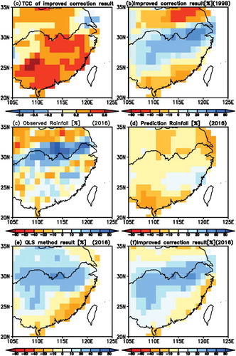
Figure 4. (a) TCCs between the observed rainfall anomaly and improved corrected result during the 30 years from 1981 to 2010. (b) Summer rainfall anomaly percentage of the improved correction results in 1998. (c) Observed summer rainfall anomaly percentage in 2016. (d) Predicted summer rainfall anomaly percentage in 2016. (e) Summer rainfall anomaly percentage of the QLS method results in 2016. (f) Summer rainfall anomaly percentage of the improved correction results in 2016.

To investigate the effect of the improved bias correction method in the real-time prediction, it is applied to correct the 2016 summer rainfall based on the 30-year hindcast data. The observed positive rainfall anomalies for summer 2016 are mainly found between the Yangtze and Yellow River basins, and the rainfall anomaly percentage can reach 60%–80% (Figure 4(c)). In contrast, the Huaihe River Basin is covered by a negative anomaly, and the abnormal rainfall characteristics in southern China are not significant.

In the uncorrected prediction result (Figure 4(d)), nearly the whole of Southeast China is characterized by negative rainfall anomalies, and the observed rainy area between the Yangtze and Yellow River basins is not captured. Besides, the rainfall anomaly percentage ranges at a low level (20%). After correcting with the QLS method, the rainy area along the Yangtze River is reproduced, and the center with strong rainfall is close to the observed position (Figure 4(e)); the PCC increases from −0.04 to 0.37. However, the anomalies in the Huaihe River Basin are still different from the observation.

Figure 4(f) shows the corrected results with the improved EOF bias correction method. Compared with the QLS method, its correction effect is even better. Not only the positive anomaly in the Yangtze River is reproduced, but the negative anomaly in the Huaihe River Basin is also well predicted. Moreover, the rainfall pattern along the Yangtze River is closer to that of the observation, and the PCC between the observation and bias-corrected prediction result reaches up to 0.59.

4. Summary and discussion

In this study, an effective improvement on the EOF-based bias correction method is proposed. The main idea is to obtain corrected PCs with better regression relationships with observed PCs by introducing stepwise regression analysis to the QLS method. Using the 30-year (1981–2010) hindcast results from IAP AGCM4.1 and CN05.1 gridded monthly rainfall data, the universality and stability of the new method are well validated. The correction effect for real-time prediction is also demonstrated, through application to the rainfall in summer 2016 as a test case.

As mentioned above, the EOF bias correction method might be model dependent. To optimize the effect of this correction method, the n and k values should be recalculated through the procedure described in section 3.2 for different models. Furthermore, a stability test of the number of hindcast modes selected for the regression is also needed, as it can greatly affect the efficiency of this method. Moreover, other topics still exist that are worthy of further investigation with respect to the EOF-based bias correction method; for instance, identification of the optimal domain size for the EOF analysis, as the dominant EOF patterns will likely vary with the region selected and the size of domain.

The EOF bias correction method demonstrates high efficiency in enhancing the prediction skill for the interannual variability of rainfall, but it might not be able to reflect the interdecadal change characteristics in the time series of PCs. Further improvement of the method could be pursued through incorporating a method that considers the interdecadal signals, e.g. the year-to-year increment approach proposed by Fan and Wang (2010).

Disclosure statement

No potential conflict of interest was reported by the authors.

Additional information

Funding

This research was jointly supported by the National Key Research and Development Program of China [grant number 2016YFC0402702], the Key Project of the Meteorological Public Welfare Research Program [grant number GYHY201406021], and the National Natural Science Foundation of China [grant numbers 41575095 and 41661144032].

References

- Chen, H., and Z. Lin. 2006. “A Correction Method Suitable for Dynamical Seasonal Prediction.” Advances in Atmospheric Sciences 23 (3): 425–430. doi:10.1007/s00376-006-0425-3.
- Christensen, J. H., F. Boberg, O. B. Christensen, and P. Lucas‐Picher. 2008. “On the Need for Bias Correction of Regional Climate Change Projections of Temperature and Precipitation.” Geophysical Research Letters 35 (20). doi:10.1029/2008GL035694.
- Fan, K., and H. Wang. 2010. “Seasonal Prediction of Summer Temperature over Northeast China Using a Year-To-Year Incremental Approach.” Acta Meteorologica Sinica 24 (3): 269–275.
- Li, F., Z. Lin, R. Zuo, and Q. Zeng. 2005. “The Methods for Correcting the Summer Precipitation Anomaly Predicted Extraseasonal over East Asian Monsoon Region Based on EOF and SVD.” Climatic and Environmental Research 10: 658–668. in Chinese.
- Li, H., J. Sheffield, and E. F. Wood. 2010. “Bias Correction of Monthly Precipitation and Temperature Fields from Intergovernmental Panel on Climate Change AR4 Models Using Equidistant Quantile Matching.” Journal of Geophysical Research: Atmospheres 115 (D10).
- Lin, Z., X. Li, Y. Zhou, G. Zhou, H. Wang, C. Yuan, Y. Guo, and Q. Zeng. 1998. “An Improved Short-Term Climate Prediction System and Its Application to the Extraseasonal Prediction of Rainfall Anomaly in China for 1998”. Climatic and Environmental Research 3 (4): 339–348. in Chinese.
- Lin, Z., Z. Yu, H. Zhang, and C. Wu. 2016. “Quantifying the Attribution of Model Bias in Simulating Summer Hot Days in China with IAP AGCM4.1.” Atmospheric and Oceanic Science Letters 9 (6): 436–442. doi:10.1080/16742834.2016.1232585.
- MacLachlan, C., A. Arribas, K. A. Peterson, A. Maidens, D. Fereday, A. A. Scaife, M. Gordon, et al. 2015. “Global Seasonal Forecast System Version 5 (Glosea5): A High‐Resolution Seasonal Forecast System.” Quarterly Journal of the Royal Meteorological Society 141 (689): 1072–1084. doi:10.1002/qj.2396.
- Qin, Z., Z. Lin, H. Chen, and Z. Sun. 2011. “The Bias Correction Methods Based on the EOF/SVD for Short-Term Climate Prediction and Their Applications.” Acta Meteorologica Sinica 69 (2): 289–296. in Chinese.
- Saha, S., S. Moorthi, H. L. Pan, and X. Wu. 2010. “The NCEP Climate Forecast System Reanalysis.” Bulletin of the American Meteorological Society 91 (8): 1015–1058. doi:10.1175/2010BAMS3001.1.
- Wang, H., K. Fan, J. Sun, S. Li, Z. Lin, G. Zhou, L. Chen, et al. 2015. “A Review of Seasonal Climate Prediction Research in China.” Advances in Atmospheric Sciences 32 (2): 149–168. doi:10.1007/s00376-014-0016-7.
- Wang, K., Z. H. Lin, J. Ling, Y. Yu, and C. L. Wu. 2016. “MJO Potential Predictability and Predictive Skill in IAP AGCM4.1.” Atmospheric and Oceanic Science Letters 9 (5): 388–393. doi:10.1080/16742834.2016.1211469.
- Wu, J., and X. Gao. 2013. “A Gridded Daily Observation Dataset over China Region and Comparison with the Other Datasets.” Chinese Journal of Geophysics 56 (4): 1102–1111. in Chinese.
- Yun, W. T., L. Stefanova, A. K. Mitra, T. S. V. Vijaya Kumar, W. Dewar, and T. N. Krishnamurti. 2005. “A Multi-Model Superensemble Algorithm for Seasonal Climate Prediction Using DEMETER Forecasts.” Tellus A 57 (3): 280–289. doi:10.3402/tellusa.v57i3.14699.
- Zeng, Q. 2009. “Progress and Challenge of the Short-Term Climate Prediction.” Atmospheric and Oceanic Science Letters 2 (5): 267–270. doi:10.1080/16742834.2009.11446820.
- Zeng, Q., B. Zhang, C. Yuan, P. Lu, F. Yang, X. Li, and H. Wang. 1994. “A Note on Some Methods Suitable for Verifying and Correcting The Prediction Of Climatic Anomaly.” Advances in Atmospheric Sciences 11 (2): 121–127. doi: 10.1007/BF02666540.
- Zeng, Q., Z. Lin, and G. Zhou. 2003. “Dynamical Extra-Seasonal Climate Prediction System IAP DCP-II.” Chinese Journal of Atmospheric Sciences 27 (3): 289–303. in Chinese.
- Zhang, H., Z. Lin, and Q. Zeng. 2009. “The Computational Scheme and the Test for Dynamical Framework of IAP AGCM-4.” Chinese Journal of Atmospheric Sciences 33: 1267–1285. in Chinese.
- Zheng, F., J. Zhu, R. Zhang, and G. Zhou. 2006. “Ensemble Hindcasts of SST Anomalies in the Tropical Pacific Using an Intermediate Coupled Model.” Geophysical Research Letters 33 (19). doi:10.1029/2006GL026994.