Evaluation of the subseasonal forecast skill of surface soil moisture in the S2S database

ABSTRACT

Based on the reforecasts from five models of the Subseasonal to Seasonal (S2S) Prediction project, the S2S prediction skill of surface soil moisture (SM) over East Asia during May–September is evaluated against ERA-Interim. Results show that good prediction skill of SM is generally 5–10 forecast days prior over southern and northeastern China in the majority of models. Over the Tibetan Plateau and northwestern China, only the ECMWF model has good prediction skill 20 days in advance. Generally, better prediction skill tends to appear over wet regions rather than dry regions. In terms of the seasonal variation of SM prediction skill, some differences are noticed among the models, but most of them show good prediction skill during September. Furthermore, the significant positive correlation between the prediction skill of SM and ENSO index indicates modulation by ENSO of the S2S prediction of SM. When there is an El Niño (a La Niña) event, the SM prediction skill over eastern China tends to be high (low). Through evaluation of the S2S prediction skill of SM in these models, it is found that the prediction skill of SM is lower than that of most atmospheric variables in S2S forecasts. Therefore, more attention needs to be given to the S2S forecasting of land processes.

Graphical Abstract

摘要

利用次季节-季节（S2S）预测计划的五个数值模式历史回报，评估了东亚5~9月土壤湿度的模式预测技巧。发现在中国南方和东北，多数S2S模式对土壤湿度的有效预测可提前5~10天；在我国青藏高原和西北地区，仅有欧洲中心模式的有效预测能提前20天左右。一般来说，土壤湿润区的预测技巧好于干燥区，多数模式在9月的预测技巧高于其余月份。然而，模式间的预测技巧还存在较大的差异。此外，厄尔尼诺-南方涛动对土壤湿度的S2S技巧也具有一定的影响，当发生厄尔尼诺（拉尼娜）事件时，我国东部的土壤湿度预测技巧偏高（低）。与大气变量相比，土壤湿度的预测技巧明显偏低，说明陆面过程的次季节预测还有待进一步的提高。

KEYWORDS:

• Soil moisture
• subseasonal to seasonal
• forecast skill evaluation
• East Asia

关键词:

• 土壤湿度；次季节；预测技巧评估
• 东亚

1. Introduction

Accurate subseasonal to seasonal (S2S) climate prediction is crucial for policy decisions (Brunet et al. 2010; White et al. 2017). However, limited S2S prediction skill based on both dynamical and statistical models makes it difficult to apply S2S prediction products to climate services (Zhang et al. 2013). In order to improve S2S prediction skill, the S2S Prediction project was sponsored by the World Meteorological Organization in 2013 (Vitart et al. 2015) and provided a comprehensive database including real-time forecasts and reforecasts on subseasonal time periods (Vitart et al. 2017). Based on the S2S products, an increasing number of studies have evaluated the prediction skill of S2S climate prediction (e.g. Vitart 2017; Jie et al. 2017; Zhou et al. 2018; Zeng and Yuan 2018).

Soil moisture (SM) is a key variable of the land surface processes. Compared to atmospheric variables, SM varies relatively slowly and anomalous SM can persist for a longer time (Entin et al. 2000). After a rainfall process, soil retains water for days or even months (Mccoll et al. 2017) and soil water exhibits evident variations on subseasonal time scales (Li et al. 2015). SM can significantly affect the energy balance, hydrological cycle, and even the atmospheric general circulation (Koster and Suarez 2000; Seneviratne et al. 2010; Mei and Wang 2011). Moreover, SM is an important predictor for the atmospheric variables in the midlatitude Northern Hemisphere during boreal summer (Liu, Yu, and Mishra 2016; Koster et al. 2017). It has been noted that the initialization of SM in numerical models can improve the performance of S2S forecasts (Koster et al. 2011). Therefore, the improvement of SM prediction could potentially improve climate prediction, especially on S2S scales.

In order to learn about the performance of current operational models to capture the SM variability on S2S scales, the S2S prediction skill of SM during the warm season (May to September) over East Asia was evaluated in this study. Section 2 describes the data and methods. The S2S forecast skill of SM is evaluated in Section 3. A summary is provided in Section 4.

2. Data and methods

Six-hourly SM data at depths of 0–7 cm and 7–28 cm, with a horizontal resolution of 1.5° × 1.5°, during 1979–2017, were obtained from the ERA-Interim reanalysis dataset (http://apps.ecmwf.int). ERA-Interim SM generally agrees with satellite and microwave observations (Rahmani, Golian, and Brocca 2016). In this study, the daily averaged surface SM at the depth of 0–20 cm was estimated by interpolating the six-hourly SM at 0–7 cm and 7–28 cm, which were weighted by distance and then averaged into daily data. Furthermore, in order to evaluate the prediction skill against different climate backgrounds, especially El Niño–Southern Oscillation (ENSO), the ENSO index during December–January of 1979–2016 was obtained from the US National Weather Service/Climate Prediction Center (http://www.cpc.ncep.noaa.gov). Although the evaluation of SM prediction skill was performed for May–September, winter ENSO index was utilized because ENSO events show their greatest strength during winter, the effects of which can persist from winter to summer.

The S2S reforecasts of SM were provided by five operational centers participating in the S2S project (http://www.s2sprediction.net/; Table 1): the Australian Bureau of Meteorology (BoM), the China Meteorological Administration (CMA), the European Centre for Medium-Range Weather Forecasts (ECMWF), the Hydrometeorological Centre of Russia (HMCR), and the US National Centers for Environmental Prediction (NCEP). Table 1 shows the land surface models (LSMs), initial conditions, and horizontal resolutions applied in the five models. In the five models, the LSMs used are the bucket model (Manabe and Holloway 1975), Noah LSM 2.7.1 (Ek et al. 2003), the Hydrology Tiled ECMWF Scheme for Surface Exchanges over Land (HTESSEL; Balsamo, Beljaars, and Scipal 2009; Balsamo et al. 2015), BCC_AVIM2 (Wu et al. 2013, 2014), and the Interactions between Soil, Biosphere, and Atmosphere scheme (ISBA; Noilhan and Planton 1989), for BoM, NCEP, ECMWF, CMA, and HMCR, respectively. The land surface variables in BoM are initialized through nudging the atmosphere model to the ERA-40 reanalysis (Hudson et al. 2011). NCEP SM is initialized by the CFSR and the Global Land Data Assimilation System (GLDAS) analyses (Saha, Moorthi, and Pan 2010). The SM of the ECMWF LSM is initialized by ERA-Interim soil reanalysis. The SM from the CMA model is not directly initialized but produced during the coupling processes of the CMA model through nudging the near-surface atmospheric forcing fields (Liu, Wu, and Yang 2017). The SM in the HMCR model is initialized through quasi-assimilation with the ERA-Interim reanalysis. The horizontal resolutions of the models range from 0.5° × 0.5° to 2° × 2°.

Table 1. The land surface model (LSM), initial conditions (Initial Con.), horizontal resolution (Hor. Res.), forecast time (Fc. Time), ensemble size (Ens. Size), reforecast frequency (Rfc. Freq.), and reforecast period (Rfc. Period) used in the five S2S models, which can be accessed at the S2S website (https://confluence.ecmwf.int/display/S2S/Models).

Model	LSM	Initial Con.	Hor. Res.	Fc. Time (days)	Ens. Size	Rfc. Freq.	Rfc. Period
BoM	Bucket model	Nudging to ERA-40	~2° × 2°	0–62	33	6/month	1981–2013
CMA	BCC_AVIM2	Not directly initialized	~1° × 1°	0–60	4	Daily	1994–2014
ECMWF	HTESSEL	ERA-I Soil reanalysis	~0.5° × 0.5°	0–46	11	2/week	1995–2014
HMCR	ISBA	Quasi-assimilation with ERA-I	~1.1° × 1.4°	0–61	10	Weekly	1985–2010
NCEP	Noah 2.7.1	CFSR and GLDAS	~1° × 1°	0–44	4	Daily	1999–2010

The forecast times, ensemble sizes, reforecast frequencies, and reforecast periods of the reforecasts of the five models are also presented in Table 1. Forecast times range from 44 to 62 days for the five models. Ensemble sizes are from 4 to 33, and reforecast frequencies are from once a week to once a day. Reforecast periods range from 20 to 32 years, and the common period of the reforecasts is 1999–2010. To present an equal evaluation for each model, reforecasts were evaluated for the period 1999–2010. However, the prediction skill during different ENSO years was analyzed during the entire period of the model reforecasts to enlarge the sample size. The horizontal resolutions of the archived data are 2.5° × 2.5° for BoM, and 1.5° × 1.5° for the rest of the models. Before evaluation, the seasonal cycles and long-term trends of both the observations and reforecasts were removed. After that, the correlation between prediction and observation was used as the prediction skill of the SM at 0–20 cm over East Asia during May–September. Note that ERA-Interim is used to assess the prediction skill of the five models because of the lack of station observations of SM. Although the same LSM (HTESSEL) is used for ERA-Interim and the ECMWF S2S reforecast, their SM results are different. The LSM in ERA-Interim is forced by ERA-Interim reanalysis data and the precipitation data of the Global Precipitation Climate Project (Balsamo, Beljaars, and Scipal 2009; Balsamo et al. 2015), while the LSM in the ECMWF S2S reforecast is coupled with the ECMWF atmospheric model. Therefore, the ERA-Interim SM is close to the observation, and it agrees well with satellite and microwave observations (Rahmani, Golian, and Brocca 2016). The SM in the ECMWF S2S reforecast is produced by the model itself, and its agreement with observation depends on the model performance.

3. SM prediction skill and its relationship with ENSO

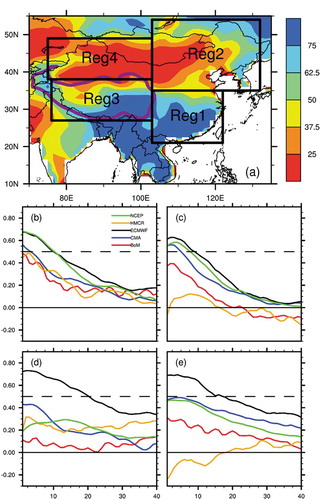
East Asia was divided into four regions by the percentile of the climatology of ERA-Interim SM (0–20 cm) during May–September of 1979–2017 (Figure 1(a)). The topography was also a factor in the division. The results show that SM decreases gradually from south to north over East Asia. Therefore, Region 1 (Reg1), mainly in southern China (21°–35°N, 103°–122°E), is the area where soil has large water content; Region 2 (Reg2), in northeastern China (35°–54°N, 103°–132°E), is a transition area where soil varies from wet to dry; Region 3 (Reg3) is the Tibetan Plateau, with the highest topography in East Asia (27°–38°N, 76°–103°E); and Region 4 (Reg4), in northwestern China (38°–49°N, 75°–103°E), has the lowest SM in East Asia.

Figure 1. (a) Percentile of the SM in the top 0–20 cm over East Asia according to ERA-Interim reanalysis. The four boxes are regions in East Asia: Reg1 (21°–35°N, 103°–122°E); Reg2 (35°–54°N, 103°–132°E); Reg3 (27°–38°N, 76°–103°E); Reg4 (38°–49°N, 75°–103°E). (b–e) Prediction skill (y-axis) of SM during the first 40 forecast-days (x-axis) in the NCEP (green line), HMCR (orange line), ECMWF (black line), CMA (blue line), and BoM (red line) models over (b) Reg1, (c) Reg2, (d) Reg3, and (e) Reg4. Prediction skill is represented by the correlation coefficient between the reforecast and observation. A good prediction skill has a correlation coefficient that is greater than 0.5.

The prediction skill of SM over Regs1–4 in BoM, CMA, ECMWF, HMCR, and NCEP are shown in Figure 1(a–d). Prediction skill is defined by the correlation coefficient between prediction and observation. The correlation coefficient is calculated based on the time series of regionally averaged SM for all the forecast cases. Generally, good prediction skill is greater than 0.5. In Figure 1, the y-axis (x-axis) is the prediction skill (forecast day). In Reg1 (Figure 1(a)), good prediction skill is found in the ECMWF and NCEP models during the first 10 forecast days. The CMA model has good skill only during the first three forecast days, while the rest of the models have no good skill. In Reg2 (Figure 1(b)), ECMWF, NCEP, and CMA have good skill before about forecast-days 10, 9, and 5, respectively. BoM and HMCR have no good skill. In Regs3 and 4 (Figure 1(c) and (d), only ECMWF has good skill during the first 20 forecast days, whereas the rest of the models have no good skill. Generally, the ECMWF model has the best prediction skill among the five models. In most of the models, prediction skill is better over wet regions than dry regions, except for the ECMWF model.

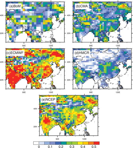
Figure 2 shows the spatial distribution of prediction skill on forecast-day 10 for the five models. In BoM (Figure 2(a)), prediction skill is higher over western Indochina, eastern China, and northeastern China than the rest of East Asia. In CMA (Figure 2(b)), good prediction skill can be found over the western Tibetan Plateau and northeastern China. In Figure 2(c), ECMWF has the best prediction skill of the five models. Moreover, good prediction skill is found over western Indochina, eastern China, northeastern China, the western Tibetan Plateau, western Mongolia, and India. In HMCR (Figure 2(d)), prediction skill is higher over central China and India than the remaining parts on the map. In NCEP (Figure 2(e)), the distribution is quite similar to that of ECMWF, but the value of prediction skill is smaller than that of ECMWF. The results shown in Figure 2 are consistent with those shown in Figure 1.

Figure 2. Prediction skill over East Asia on forecast-day 10 for (a) BoM, (b) CMA, (c) ECMWF, (d) HMCR, and (e) NCEP.

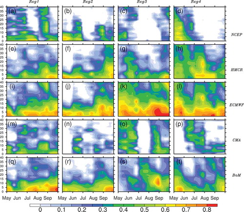
Besides spatial distribution, the prediction skill of SM has seasonal variation. Figure 3 presents the temporal variation of SM prediction skill over the four regions in the five models. In BoM (Figure 3(a–d)), SM can be well predicted five days in advance during July in Reg1, 10 days during May in Reg2, and 25 days during May in Reg4. In Reg3, BoM has no good skill during May–September. CMA has good prediction skill 10 forecast-days in advance in Reg1 (Figure 3(e)). In Reg2 (Figure 3(f)), good prediction skill is found before forecast-day 5 (20) during May–June (August–September). In Reg3 (Reg4), SM can be well predicted 5 (20) days in advance during June–July and September (May and July–August) in Figure 3(g) (Figure 3(h)). ECMWF generally has good prediction skill before forecast-day 10–15 during May–August (Figure 3(i–l)). In Regs3 and 4 (Figure 3(k) and (l), good prediction skill is before forecast-day 20–25. In HMCR, good prediction skill can be found before forecast-day 5 (10) during June (August) in Reg1 (Reg3) in Figure 3(m) (Figure 3(o)). In Regs2 and 4 (Figure 3(n) and (p), no good prediction skill can be found during May–September. In NCEP, good prediction skill is before forecast-day 10 during May–September over Regs1 and 2 (Figure 3(q) and (r). In Reg3 (Reg4), SM is well predicted 20 days in advance during August to September (May and September) in Figure 3(s) (Figure 3(t)). Overall, the seasonal variation of SM prediction shows large diversity in the five models, which indicates some uncertainties exist in the prediction skill of SM among the five models. However, a common feature can also be identified in that good prediction skill tends to be found in September over most of the regions in most of the models.

Figure 3. Temporal variation of the prediction skill of SM (shading) over each region (columns) in each model (rows). Prediction skill is calculated in 10-day bins during may–september (x-axis) at each forecast time (y-axis) to obtain the temporal variation.

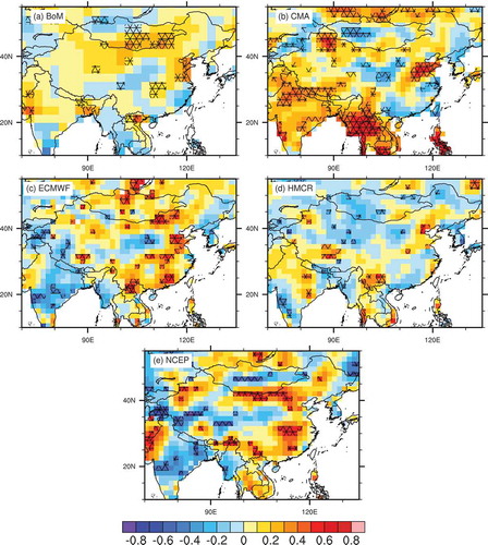
The prediction skill related to ENSO was also evaluated because the S2S prediction skill of SM can be modulated by ENSO. The results are shown in Figure 4 in the form of the correlation coefficients between the annual prediction skill and ENSO index at each grid point. The prediction skill on forecast-day 10 correlated with ENSO is shown because the correlation patterns between ENSO index and prediction skill during the first 15 forecast days are very similar. Moreover, forecast-day 10 is the start of the S2S forecast. In BoM (Figure 4(a)), a region that generally features significant positive correlation is located from northern Indochina to Shandong Province of China. Correlations are also significantly positive over northern China and eastern Mongolia. In CMA (Figure 4(b)), positive correlation can be identified over northern India, the Indochina Peninsula, Shandong Province, and northern Xinjiang. In ECMWF (Figure 4(c)), correlations are generally significantly positive from northern Indochina to Shandong Province and northern China. In HMCR (Figure 4(d)), positive and significant correlations are found over southwestern China, part of the Tibetan Plateau, and a small part of northern China. The correlation pattern shown in NCEP (Figure 4(e)) is quite similar to those shown in BoM and ECMWF. In general, except for HMCR, the prediction skill of SM from southwestern China to Shandong Province is significantly correlated with ENSO index in all the models. This indicates that SM prediction is better in El Niño years than La Niña years.

Figure 4. Correlation between ENSO index in winter (december–january–february) and SM prediction skill at the forecast time of 10 days during may–september. Grid cells marked with asterisks are significant at the 0.1 level based on the student’s t-test.

4. Summary

Using the SM at the depth of 0–20 cm derived from the S2S Prediction project database, the S2S prediction skill of SM in East Asia during May–September was evaluated against ERA-Interim reanalysis data. Most of the five models provide good prediction skill at 5–10 days in advance over southern China and northeastern China. Over the Tibetan Plateau and northwestern China, only the ECMWF model has good prediction skill at about 20 forecast-days in advance. However, observations are very limited over the Tibetan Plateau, and therefore prediction here may not be very reliable. Generally, good prediction skill is found over wet regions rather than dry regions in most of the models. This may relate to the long ‘memory’ of SM over wet regions. For the seasonal variation of SM prediction skill, some uncertainties can be noticed, but most of the models show good prediction skill during September. This may be attributable to the fact that the rainy season over East Asia usually takes place before September, which makes the soil wet; after that, rainfall reduces and, due to the memory of SM, the persistence of anomalous SM may lead to good prediction skill. Except for the HMCR model, all the S2S models show that the prediction skill of SM over eastern China is significantly and positively correlated with ENSO index, which means SM predictions are better during El Niño years than La Niña years. Comparing this study to others (e.g. Zhou et al. 2018), it is apparent that the prediction skill of SM is lower than that for most atmospheric variables in the S2S forecast. This indicates that more attention should be paid to the subseasonal forecasting of land processes.

Correction Statement

This article has been republished with minor changes. These changes do not impact the academic content of the article.

Acknowledgments

Yang ZHOU thanks the support from the Startup Foundation for Introducing Talent of NUIST. Finally, we thank the reviewers for their insightful and constructive comments. We thank Ms. Chuyan CHEN for proofreading the manuscript.

Disclosure statement

No potential conflict of interest was reported by the authors.

Additional information

Funding

This study was supported by the National Key R&D Program of China [grant number 2016YFA0602100].

References

- Balsamo, G., C. Albergel, A. Beljaars, S. Boussetta, E. Brun, H. Cloke, D. Dee, et al. 2015. “ERA-Interim/Land: A Global Land Surface Reanalysis Data Set.” Hydrology and Earth System Sciences 19 :389–407. doi:10.5194/hess-19389-2015.
- Balsamo, G., A. Beljaars, and K. Scipal. 2009. “A Revised Hydrology for the ECMWF Model: Verification from Field Site to Terrestrial Water Storage and Impact in the Integrated Forecast System.” Journal of Hydrometeorology 10 (3): 623. doi:10.1175/2008JHM1068.1.
- Brunet, G., M. Shapiro, B. Hoskins, M. Moncrieff, R. Dole, G. N. Kiladis, B. Kirtman, et al. 2010. “Collaboration of the Weather and Climate Communities to Advance Subseasonal-to-seasonal Prediction.” Bulletin of the American Meteorological Society 91 (10): 1397–1406. doi:10.1175/2010BAMS3013.1.
- Ek, M. B., K. E. Mitchell, Y. Lin, E. Rogers, P. Grunmann, V. Koren, G. Gayno, and J. D. Tarpley. 2003. “Implementation of Noah Land Surface Model Advances in the National Centers for Environmental Prediction Operational Mesoscale Eta Model.” Journal of Geophysical Research 108 (D22): 8851. doi:10.1029/2002JD003296.
- Entin, J. K., A. Robock, K. Y. Vinnikov, S. E. Hollinger, S. Liu, and A. Namkhai. 2000. “Temporal and Spatial Scales of Observed Soil Moisture Variations in the Extratropics.” Journal of Geophysical Research Atmospheres 105 (D9): 11865–11877. doi:10.1029/2000JD900051.
- Hudson, D., O. Alves, H. H. Hendon, and G. Wang. 2011. “The Impact of Atmospheric Initialisation on Seasonal Prediction of Tropical Pacific SST.” Climate Dynamics 36: 1155–1171. doi:10.1007/s00382-010-0763-9.
- Jie, W., F. Vitart, T. Wu, and X. Liu. 2017. “Simulations of Asian Summer Monsoon in the Sub-Seasonal to Seasonal Prediction Project (S2S) Database: Simulations of Asian Summer Monsoon in the S2S Database.” Quarterly Journal of the Royal Meteorological Society 143: 2282–2295. doi:10.1002/qj.3085.
- Koster, R. D., A. K. Betts, P. A. Dirmeyer, M. Bierkens, K. E. Bennett, S. J. Déry, J. P. Evans, et al. 2017. “Hydroclimatic Variability and Predictability: A Survey of Recent Research.” Hydrology and Earth System Sciences 21 (7): 3777–3798. doi:10.5194/hess-21-3777-2017.
- Koster, R. D., S. P. P. Mahanama, T. J. Yamada, G. Balsamo, A. A. Berg, M. Boisserie, P. A. Dirmeyer, et al. 2011. “The Second Phase of the Global Land–Atmosphere Coupling Experiment: Soil Moisture Contributions to Subseasonal Forecast Skill.” Journal of Hydrometeorology 12 (5): 805–822. doi:10.1175/2011JHM1365.1.
- Koster, R. D., and M. J. Suarez. 2000. “Soil Moisture Memory in Climate Models.” Journal of Hydrometeorology 2 (6): 558–570. doi:10.1175/1525-7541(2001)002<0558:SMMICM>2.0.CO;2.
- Li, J. Y., A. Kokkinaki, H. Ghorbanidehno, E. F. Darve, and P. K. Kitanidis. 2015. “The Compressed State Kalman Filter for Nonlinear State Estimation: Application to Large-scale Reservoir Monitoring.” Water Resources Research 51 (12): 9942–9963. doi:10.1002/2015WR017203.
- Liu, D., Z. Yu, and A. K. Mishra. 2016. “Evaluation of Soil Moisture-precipitation Feedback at Different Time Scales over Asia.” International Journal of Climatology 37: 3619–3629. doi:10.1002/joc.4943.
- Liu, X., T. Wu, and S. Yang. 2017. “MJO Prediction Using the Sub-Seasonal to Seasonal Forecast Model of Beijing Climate Center.” Climate Dynamics 48: 3283–3307. doi:10.1007/s00382-016-3264-7.
- Manabe, S., and J. L. Holloway Jr. 1975. “The Seasonal Variations of the Hydrologic Cycle as Simulated by a Global Model of the Atmosphere.” Geophysical Research 80: 1617–1649. doi:10.1029/JC080i012p01617.
- Mccoll, K. A., S. H. Alemohammad, R. Akbar, A. G. Konings, S. Yueh, and D. Entekhabi. 2017. “The Global Distribution and Dynamics of Surface Soil Moisture.” Nature Geoscience 10 (2): 100–104. doi:10.1038/ngeo2868.
- Mei, R., and G. Wang. 2011. “Impact of Sea Surface Temperature and Soil Moisture on Summer Precipitation in the United States Based on Observational Data.” Journal of Hydrometeorology 12 (5): 1086–1099. doi:10.1175/2011JHM1312.1.
- Noilhan, J., and S. Planton. 1989. “A Simple Parameterization of Land Surface Processes for Meteorological Models.” Monthly Weather Review 117: 536–549. doi:10.1175/1520-0493(1989)117<0536:ASPOLS>2.0.CO;2.
- Rahmani, A., S. Golian, and L. Brocca. 2016. “Multiyear Monitoring of Soil Moisture over Iran through Satellite and Reanalysis Soil Moisture Products.” International Journal of Applied Earth Observations & Geoinformation 48: 85–95. doi:10.1016/j.jag.2015.06.009.
- Saha, S., S. Moorthi, and H.-L. Pan. 2010. “The NCEP Climate Forecast System Reanalysis.” Bulletin of the American Meteorological Society 91: 1015–1057. doi:10.1175/2010BAMS3001.1.
- Seneviratne, S. I., T. Corti, E. L. Davin, M. Hirschi, E. B. Jaeger, I. Lehner, B. Orlowsky, and A. J. Teuling. 2010. “Investigating Soil Moisture–Climate Interactions in A Changing Climate: A Review.” Earth Science Reviews 99 (3): 125–161. doi:10.1016/j.earscirev.2010.02.004.
- Vitart, F. 2017. “Madden-Julian Oscillation Prediction and Teleconnections in the S2S Database.” Quarterly Journal of the Royal Meteorological Society 143: 2210–2220. doi:10.1002/qj.3079.
- Vitart, F., C. Ardilouze, A. Bounet, A. Brookshaw, M. Chen, C. Codorean, M. Deque, et al. 2017. “The Subseasonal to Seasonal (S2S) Prediction Project Database.” Bulletin of the American Meteorological Society 98: 163–173. doi:10.1175/BAMS-D-16-0017.1.
- Vitart, F., A. W. Robertson, and S2S Steering Group. 2015. “Sub-Seasonal to Seasonal Prediction: Linking Weather and Climate.” Chapter 20 in Seamless Prediction of the Earth System: From Minutes to Months. G. Brunet, S. Jones, and P. M. Ruti, Eds., WMO- No 1156, World Meteorological Organization, 385–401.
- White, C. J., H. Carlsen, A. W. Robertson, R. J. Klein, J. K. Lazo, A. Kumar, F. Vitart, et al. 2017. “Potential Applications of Subseasoanl-to Seasonal (S2S) Predictions.” Meteorological Applications 24: 315–325. doi:10.1002/met.1654.
- Wu, T., W. Li, J. Ji, X. Xin, L. Li, Z. Wang, Y. Zhang, et al. 2013. “Global Carbon Budgets Simulated by the Beijing Climate Center Climate System Model for the Last Century.” Journal of Geophysical Research Atmospheres 118: 4326–4347. doi:10.1002/jgrd.50320.
- Wu, T., L. Song, W. Li, Z. Wang, H. Zhang, X. Xin, Y. Zhang, et al. 2014. “An Overview of BCC Climate System Model Development and Application for Climate Change Studies.” Journal of Meteorological Research 28(1): 34–56. doi:10.1007/s13351-014-3041-7.
- Zeng, D., and X. Yuan. 2018. “Multiscale Land–Atmosphere Coupling and Its Application in Assessing Subseasonal Forecasts over East Asia.” Journal of Hydrometeorology 19 (5): 745–760. doi:10.1175/JHM-D-17-0215.1.
- Zhang, C., J. Gottschalck, E. D. Maloney, M. W. Moncrieff, F. Vitart, D. E. Waliser, B. Wang, and M. C. Wheeler. 2013. “Cracking the MJO Nut.” Geophysical Research Letters 40 (6): 1223–1230. doi:10.1002/grl.50244.
- Zhou, Y., B. Yang, H. Chen, Y. Zhang, A. Huang, and M. La. 2018. “Effects of the Madden–Julian Oscillation on 2-m Air Temperature Prediction over China during Boreal Winter in the S2S Database.” Climate Dynamics 52: 6671–6689. doi:10.1007/s00382-018-4538-z.