Comparison of two double-moment microphysics schemes in aspects of warm-rain droplet spectra and raindrop budget

ABSTRACT

Simulation results of the WDM6 scheme and the Thompson scheme, both of which are commonly-used double-moment bulk microphysics schemes, are compared within the Weather Research and Forecasting model. The purpose of the comparison is to study the difference in the aspects of the warm-rain hydrometeor number concentrations, the droplet size distributions, and the budgets of the rain mixing ratio and number concentration. It is found that the WDM6 scheme overestimates the ratio and the amount of large precipitation, and underestimates those of small precipitation, compared to the Thompson scheme. The cloud number concentration (CNC) predicted in the WDM6 scheme is one to three orders of magnitude smaller than that of the Thompson scheme, which is set to the specific value of CNC. The cloud droplet spectra of the WDM6 scheme are broader. The WDM6 scheme produces a larger rain number concentration and smaller mass mean diameter of raindrops under the influence of both warm and cold rain processes— specifically, autoconversion and melting of snow and graupel. The WDM6 scheme produces a larger autoconversion rate and smaller total melting rate of snow and graupel than the Thompson scheme in the rain mixing ratio budget. The sign of the difference in the rain-cloud collection varies with region, and the rain-cloud collection process together with evaporation of rain have a major influence on the sign of the surface precipitation difference between the two schemes.

Graphical abstract

摘要

本文对WRF模式中两种常用的雨滴双参数微物理方案，即Thompson方案和WDM6方案在华北地区‘7.20’暴雨中暖云粒子谱和雨滴源汇项的模拟差异，以及上述差异如何影响降水模拟进行了详细的分析。结果表明：WDM6方案模拟的云滴数浓度比Thompson方案中给定的云滴数浓度概量小1-3个量级，云滴谱较宽。云雨自动转换过程和雪、霰融化过程的共同导致WDM6方案雨滴粒子数浓度较大，平均尺度较小。本文着眼于微物理方案间的暖云粒子谱模拟差异，是以往研究关注较少的领域，有助于更好地理解微物理方案的模拟特征。

KEYWORDS:

• WDM6 scheme
• Thompson scheme
• droplet number concentration
• droplet size distribution
• raindrop budget analysis

关键词:

• WDM6方案
• Thompson方案
• 粒子数浓度
• 粒子谱分布
• 雨滴源汇项分析

1. Introduction

Microphysics parameterization determines the evolution of hydrometeors, affects latent heat release, and interacts with dynamics. Thus, microphysics parameterization plays a central role in the prediction of the occurrence, development, and dissipation of weather systems. Double-moment schemes (Reisner, Rasmussen, and Bruintjes 1998; Cohard and Pinty 2000; Seifert and Beheng 2001; Morrison, Curry, and Khvorostyanov 2005; Thompson et al. 2008), which typically predict the number concentration in addition to the mixing ratio of hydrometeors, offer a more flexible treatment of droplet size distributions (DSDs), and outperform their single-moment counterparts (Morrison, Thompson, and Tatarskii 2009; Lim and Hong 2010; Jung, Xue, and Tong 2012). Double-moment schemes show advantage in the capability of investigating interactions of cloud and aerosols, e.g. in the Weather Research and Forecasting (WRF) model (Xie et al. 2013) and the Community Atmosphere model, version 5 (Xie et al. 2017).

Sensitivity tests of the simulation of microphysics schemes have been conducted for various weather systems. Different treatments of graupel and hail were found by Morrison and Milbrandt (2011) to be responsible for the differences in aspects of storm dynamics, reflectivity structure, surface precipitation, and cold pool between two microphysics schemes. Adams-Selin, van Den Heever, and Johnson (2013) tested the sensitivity of a bow-echo simulation to eight microphysics schemes in aspects of rainfall, radar reflectivity, and hydrometeor mixing ratio, among others, with a focus on graupel parameter characteristics. The sensitivity of the simulation of tropical cyclone size to microphysics schemes was tested by Chan and Chan (2016). Simulations of different microphysics schemes were compared with remote-sensing observations with respect to the aspects of reflectivity, differential reflectivity, and microwave brightness temperature, among others, to analyze the characteristics of droplet spectra without explaining the cause of droplet spectra differences (Gao et al. 2011; Jankov et al. 2011; Molthan and Colle 2012; Johnson et al. 2016). However, few of these studies concentrated on droplet number concentrations, spectra and identifying microphysical causes of differences between microphysics schemes.

The objective of this paper is to explore the differences in droplet spectra and the microphysical causes of the differences between two commonly used double-moment bulk schemes in the WRF model (Skamarock and Klemp 2008) through a budget analysis.

2. Model configuration

During 19–21 July 2016, continuous heavy rain that mainly affected the provinces of Beijing, Tianjin, Hebei, Henan, Shandong, Shanxi, and Liaoning occurred in North China. The average accumulated precipitation from 1700 UTC 18 July to 0000 UTC 21 July in Beijing was 212.6 mm.

The WDM6 scheme (Lim and Hong 2010) and the Thompson scheme (Thompson et al. 2008) are used in this study. These schemes were chosen because they have been widely used and tested (e.g. Loughner et al. 2011; Bove et al. 2014; Clark et al. 2014; Varble et al. 2014), and the main point of interest of the study is their different treatment of cloud number concentration (CNC). Both schemes predict the mixing ratio of cloud, rain, ice, snow, graupel, and the number concentration of rain. Additionally, the WDM6 scheme predicts the number concentration of cloud condensation nuclei (CCN) and clouds, while the Thompson scheme predicts the number concentration of ice and sets the CNC as a constant. The gamma distribution,

(1) $n(D)=N_0{D}^{\alpha }exp(-\lambda D),$(1)

and the four-parameter normalized gamma function,

(2) $n(D)=N\frac{\alpha }{\mathrm{\Gamma }(\nu )}{\lambda }^{\alpha \nu }{D}^{\alpha v-1}exp[-(\lambda D{)}^{\alpha }],$(2)

are adopted for rain DSD in the Thompson scheme and the WDM6 scheme, respectively. Here, λ is the slope parameter, whereas α and ν are the dispersion parameters. Besides, N, N₀, and D represent the droplet number concentration, intercept parameter, and diameter of droplets, respectively. Additional details of parameter definitions of the schemes are presented in Tables 1 and 2. The simulations performed using the WRF model (version 3.6) cover the 18-h period from 0000 to 1800 UTC 20 July, during which time precipitation was mainly located in Beijing. The model setup is shown in Table 3.

Table 1. Parameter definitions in the Thompson microphysics scheme. The fall speed relation for the Thompson scheme is $V(D)=\gamma c{D}^{d}exp(-fD)$, in which $\gamma =({\rho }_0/{\rho }_{\mathrm{a}\mathrm{i}\mathrm{r}}{)}^{0.5}$ and ρ₀ is the standard air density at sea level. The mass relation is $m=a{D}^b$.

Species	N0	α	ρ	a	b	c	d	f
Cloud	3 × 10^8	5	1000	πρw/6	3	0.316946 × 10^8	2	0
Rain	Prognostic	0	1000	πρw/6	3	4854	1	195
Ice	Prognostic	0.6357	890	πρi/6	2	1847.5	1	0
Graupel	10^4－3 × 10^6	0	500	πρg/6	3	442	0.89	0
Snow	Temperature dependent	0	100	0.069	2	40	0.55	100

Table 2. Parameter definitions in the WDM6 microphysics scheme. The fall speed relation for the WDM6 scheme is $V(D)=c{D}^d$. The particle size distribution of the WDM6 scheme is $n(D)=N\frac{\alpha }{\mathrm{\Gamma }(\nu )}{\lambda }^{\alpha \nu }{D}^{\alpha v-1}exp[-(\lambda D{)}^{\alpha }]$. The mass relation is $m=a{D}^b$.

Species	N0	α	ν	ρ	a	b	c	d
Cloud	Prognostic	3	1	1000	πρw/6	3	–	–
Rain	Prognostic	1	2	1000	πρw/6	3	841.9γ	0.8
Ice	–	–	–	–	0.2899	2	1.49 × 10^4	1.31
Graupel	4 × 10^6	1	1	500	πρg/6	3	330γ	0.8
Snow	Temperature dependent	1	1	100	πρs/6	3	11.72γ	0.41

Table 3. Model configuration.

	Outer domain	Inner domain
Grids	151 × 130, 9 km, 40 layers	196 × 199, 3 km, 40 layers
Cumulus	Kain–Fritsch	None
Radiation	RRTM longwave, Dudhia shortwave
Land surface	NOAH-MP
Surface layer	Revised MM5
PBL	YSU
Microphysics	WDM6 or Thompson

3. Model simulation results

3.1 Precipitation

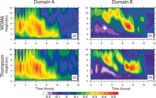
The simulated 0000–1800 UTC accumulated precipitation is presented in Figure 1(a,b). Generally, simulation using either scheme agrees with the observations (Figure 1(d)) in location. Both simulations have a rainfall center of over 300 mm in central Beijing and the simulated accumulated precipitation of both schemes is larger than the observations. The probability distribution of hourly precipitation of the Thompson scheme is closer to the observation than that of the WDM6 scheme. The WDM6 scheme underestimates the ratio of precipitation smaller than 5 mm h⁻¹ and overestimates the ratio of larger precipitation at the same time (Figure 1(f)). As shown in Table 4, the average precipitation is larger when the WDM6 scheme produces more precipitation. Meanwhile, the WDM6 scheme overestimates larger precipitation and underestimates smaller precipitation compared to the observation. Two typical domains (marked as domain A and B in Figure 1(c)) around Beijing are chosen to explore the differences and the corresponding microphysical causes in hydrometeor characteristics between the two schemes. The simulated radar reflectivity of both schemes compares well with the observation in domain A. However, the WDM6 scheme shows a delay of precipitation in domain B, as presented in Figure 2. In domain A, the WDM6 scheme generally produces more precipitation than the Thompson scheme, while the opposite happens in domain B. Domain A is mainly dominated by updrafts, with a maximum average vertical velocity exceeding 0.5 m s⁻¹. Downdrafts are dominant at a lower level in domain B in both schemes, as shown in Figure 3.

Table 4. Average accumulated precipitation (units: mm) of the WDM6 scheme simulation, the Thompson scheme simulation, and the observation in different regions.

Region	WDM6	Thompson	Observation
WDM6 > Thompson	64.83	51.35	56.37
WDM6 ≤ Thompson	29.61	37.66	37.86

Figure 1. Accumulated precipitation during 0000–1800 UTC in the (a) WDM6 scheme simulation, (b) Thompson scheme simulation, (c) their difference (WDM6 minus Thompson), and (d) observations. (f) Probability distribution function (PDF) of hourly precipitation.

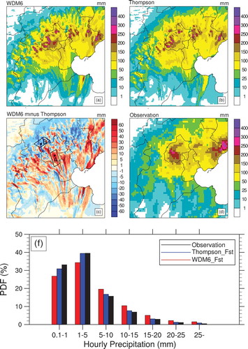
Figure 2. Time–height series of median observed Beijing S-band radar (39.81°N, 116.47°E) and simulated radar reflectivity (units: dBZ): (a) observations in domain A; (b) observations in domain B; (c) WDM6 scheme simulation in domain A; (d) WDM6 scheme simulation in domain B; (e) Thompson scheme simulation in domain A; (f) Thompson scheme simulation in domain B.

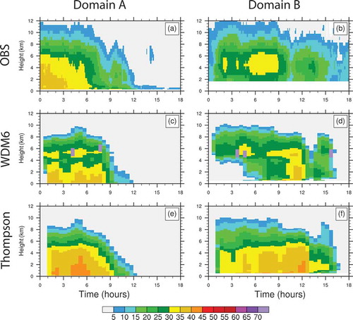
Figure 3. Time–height series of average vertical velocity (units: m s⁻¹): (a) WDM6 scheme simulation in domain A; (b) WDM6 scheme simulation in domain B; (c) Thompson scheme simulation in domain A; (d) Thompson simulation in domain B.

3.2 Hydrometeors

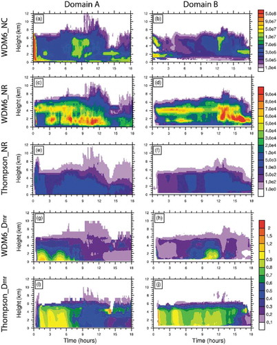
Time–height series of the warm-rain hydrometeor number concentrations of the two schemes are presented in Figure (4a–f). The treatment of CNC is quite different between the two schemes. In the Thompson scheme, the CNC is set at a constant of 3 × 10⁸ m⁻³, as recommended for a continental system. However, in the WDM6 scheme, the CNC is predicted with an initial CCN number concentration (CNNC) of 10⁹ m⁻³ (Yum and Hudson 2002). We also tested the WDM6 scheme with an initial CNNC of 10¹⁰ m⁻³, since the CNNC is about 10⁹–10¹⁰ m⁻³ at a supersaturation of 0.4%–0.6% according to observations in North China (Shi and Duan 2007; Deng et al. 2011; Li et al. 2015). The results, which are not presented here, showed that the simulation is more sensitive in the choice of microphysics scheme than the initial CNNC. The CNC in the WDM6 scheme is within the range of 10⁵–10⁷ m⁻³, which is one to three orders of magnitude smaller than the typical CNC magnitude of 10⁸ m⁻³ (Huang and Xu 1999), except during 0000–0100 UTC. The rain number concentration (RNC) in the WDM6 scheme, with two maxima at 2 km and 5 km, is over 10 times higher than that in the Thompson scheme.

Figure 4. Time–height series of average warm-rain droplet number concentration (units: m⁻³) and median mean mass diameter of raindrops (units: mm): (a) CNC in domain A in the WDM6 scheme; (b) CNC in domain B in the WDM6 scheme; (c) RNC in domain A in the WDM6 scheme; (d) RNC in domain B in the WDM6 scheme; (e) RNC in domain A in the Thompson scheme; (f) RNC in domain B in the Thompson scheme; (g) median mean mass diameter of raindrops in domain A in the WDM6 scheme; (h) median mean mass diameter of raindrops in domain B in the WDM6 scheme; (i) median mean mass diameter of raindrops in domain A in the Thompson scheme; (j) median mean mass diameter of raindrops in domain B in the Thompson scheme.

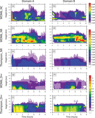
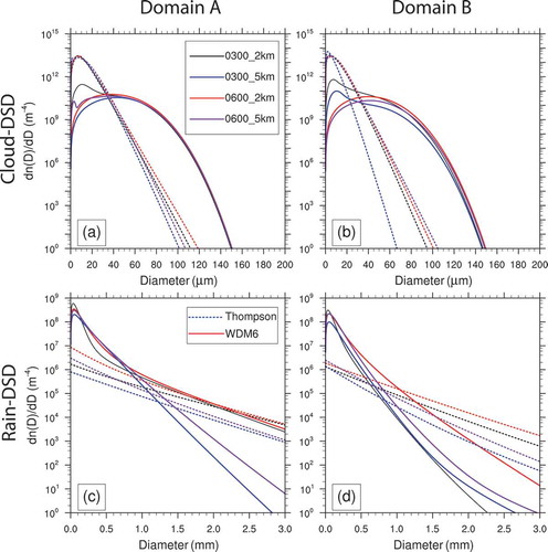
There is also a notable difference in the warm-rain DSD between the two schemes. The DSDs are explicitly predicted in bin schemes, whereas they are calculated by the number concentration, mixing ratio, and the predefined DSD forms in bulk schemes. The warm-rain DSDs of 0300 UTC and 0600 UTC at 2 km and 5 km are taken as examples and shown in Figure 5. It is found that the WDM6 scheme produces wider cloud spectra, with more cloud droplets of 30 μm in diameter or larger. Meanwhile, the raindrop spectra are narrower in the WDM6 scheme, and numerous small raindrops with diameters of approximately 0.1 mm are responsible for the larger RNC. It has also been found, in other research, that the WDM6 scheme tends to produce a large RNC and a high proportion of small raindrops (Gao et al. 2011; Adams-Selin, van Den Heever, and Johnson 2013; Morrison et al. 2015; Johnson et al. 2016). The mean mass diameter of raindrops (D_mr) influences the terminal velocity, radar reflectivity, and microphysical processes of evaporation, collection, etc. Time–height series of the median D_mr are presented in Figure 4(g–j). As can be seen, D_mr increases while descending to the ground in both schemes during most simulation periods, which demonstrates the ability of reflecting ‘size-sorting’ in double-moment microphysics schemes. Generally, the D_mr of the WDM6 scheme is smaller and varies more widely with altitude.

Figure 5. Average droplet spectra of warm-rain hydrometeors of 0300 UTC and 0600 UTC at 2 km and 5 km, with the results of the WDM6 scheme and the Thompson scheme presented by the solid line and dashed line, respectively: (a) cloud spectrum in domain A; (b) cloud spectrum in domain B; (c) rain spectrum in domain A; (d) rain spectrum in domain B.

3.3 Budget analysis of raindrops

Vertical profiles of horizontally averaged and temporally averaged budget terms of RNC and rain mixing ratio between 0100 and 1400 UTC in domain A and B are presented in Figure 6. The period 0100–1400 UTC is chosen because the rainfall rate is quite different in the two schemes in both domains during this period.

Figure 6. Average profiles of the budget terms of the (a–d) RNC (units: m⁻³ s⁻¹) and (e–j) rain mixing ratio (units: 10⁻⁶ kg kg⁻¹ s⁻¹). The first and third rows represent the results in domain A. The second and fourth rows represent the results in domain B. The first, second, and third columns represent the results of the WDM6 scheme, the Thompson scheme, and the difference between them (WDM6 minus Thompson), respectively.

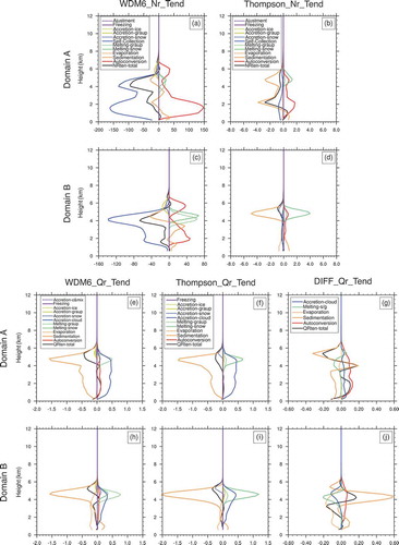
There is a more significant difference in the budget terms of RNC than that of rain mixing ratio between the two schemes. The main sources of RNC include autoconversion (Autoconversion in Figure 6) and melting of snow and graupel (Melting-snow and Melting-graup in Figure 6; hereafter, Melt_sg), and all of these terms are larger in the WDM6 scheme. Autoconversion is the process of collision and coalescence of cloud droplets to form raindrops. The autoconversion rate of the RNC in the WDM6 scheme is one to three orders of magnitude larger than in the Thompson scheme. The parameterization of autoconversion, which is positively associated with five power of cloud droplet diameter, follows Cohard and Pinty (2000) in both MP schemes. Thus, the larger autoconversion rate is a result of the wider cloud spectra produced by the WDM6 scheme. Melt_sg is responsible for the maximum RNC at approximately 5 km (Figure 4(c,d)) in the WDM6 scheme. The rain mixing ratio produced by Melt_sg is similar in magnitude, and thus the difference in the RNC source of Melt_sg is caused by the different treatment of snow and graupel number concentrations between the two schemes. Self-collection/breakup (Self-Collection in Figure 6), which is the process of raindrops collecting other raindrops or breaking up after collision, is the main sink of the RNC and forms a negative feedback effect on the larger RNC.

The rain mixing ratio is mainly increased by rain-collecting cloud droplets (Accretion-Cloud in Figure 6) and Melt_sg, and decreased by falling to the ground (Sedimentation in Figure 6). In domain A, rain-cloud collection is comparable with Melt_sg, while Melt_sg is the dominant source of the rain mixing ratio in domain B in both schemes. Evaporation of raindrops is vigorous in domain B, especially in the WDM6 scheme. Autoconversion is an important source of the RNC, while it contributes little to the rain mixing ratio, indicating that the raindrop size produced by autoconversion is much smaller than that produced by Melt_sg. The term Accretion-c&mix in the WDM6 scheme represents the process of clouds collected by snow and graupel in a warm area converting to rain, which could be considered another form of Melt_sg.

The differences in the main budget terms of the rain mixing ratio between the two schemes (WDM6 minus Thompson) are presented in Figure 6(g,j). The melting of snow and graupel are treated as one term because they are similar, and the Accretion-c&mix term of the WDM6 scheme is also regarded as the melting of snow and graupel. In the Thompson scheme, Melt_sg is larger in the rain mixing ratio budget, while it is smaller in RNC budget in both domain A and B, indicating the D_mr of raindrops produced by Melt_sg is larger in the Thompson scheme than that of the WDM6 scheme. As discussed previously, the autoconversion process produces a large number of small raindrops. Vigorous autoconversion in the WDM6 scheme is another reason for the smaller D_mr. Rain-cloud collection does not change the RNC, which leads to an increase in the D_mr. Rain-cloud collection is found to be larger in the WDM6 scheme in domain A, making D_mr in the WDM6 scheme comparable with that in the Thompson scheme. In domain B, evaporation is larger due to the larger total surface area of numerous smaller raindrops in the WDM6 scheme. Besides, rain-cloud collection is smaller, and thus the D_mr is much smaller in the WDM6 scheme. As a result, precipitation is smaller in the WDM6 scheme in domain B. The difference in rain-cloud collection could be an explanation of the overestimation of large precipitation and underestimation of small precipitation.

4. Summary

In this study, the WDM6 scheme and the Thompson scheme, both of which are double-moment schemes for raindrops, are compared in a simulation of an unusually heavy rainfall event in North China on 20 July 2016. Although the simulation basically agrees with observations in terms of rainfall location and accumulated precipitation when either of the two schemes is used, there are notable differences in the aspects of surface precipitation, warm-rain DSDs and droplet number concentration, among others. The major conclusions can be summarized as follows:

The probability distribution of the hourly precipitation of the Thompson scheme is closer to the observations than that of the WDM6 scheme. The WDM6 scheme overestimates (underestimates) the ratio and amount of large (small) precipitation.

The CNC is predicted in the WDM6 scheme but is set as constant in the Thompson scheme. The WDM6 scheme produces a much smaller CNC and wider cloud droplet spectra compared to the Thompson scheme.

The WDM6 scheme produces over 10 times more raindrops than the Thompson scheme, as a result of both a larger rate of autoconversion and melting of snow and graupel. The raindrop spectra are narrower, and numerous raindrops with diameters of 0.1 mm are responsible for the larger RNC in the WDM6 scheme.

For the rain mixing ratio budget terms, the WDM6 scheme produces a larger autoconversion rate and smaller total melting rate of snow and graupel than the Thompson scheme. The rain-cloud collection rate is larger in the WDM6 scheme in the area dominated by updrafts. As a result, a large number of small raindrops develop by collecting cloud droplets, leading to more precipitation in the WDM6 scheme. Meanwhile, in the area where convection is not vigorous, the precipitation of the WDM6 scheme is less than that of the Thompson scheme. The reason could be the smaller rain-cloud collection term and the larger evaporation rate owing to the larger total surface area of numerous small raindrops.

Disclosure statement

No potential conflict of interest was reported by the authors.

Additional information

Funding

This study was sponsored by the National Natural Science Foundation of China [grant number 41530427].

References

- Adams-Selin, R. D., S. C. van Den Heever, and R. H. Johnson. 2013. “Sensitivity of Bow-Echo Simulation to Microphysical Parameterizations.” Weather and Forecasting 28 (5): 1188–1209. doi:10.1175/WAF-D-12-00108.1.
- Bove, M. C., P. Brotto, F. Cassola, E. Cuccia, D. Massabò, A. Mazzino, A. Piazzalunga, and P. Prati. 2014. “An Integrated PM2.5 Source Apportionment Study: Positive Matrix Factorisation Vs. The Chemical Transport Model CAMx.” Atmospheric Environment 94: 274–286. doi:10.1016/j.atmosenv.2014.05.039.
- Chan, K. T. F., and J. C. L. Chan. 2016. “Sensitivity of the Simulation of Tropical Cyclone Size to Microphysics Schemes.” Advances in Atmospheric Sciences 33 (9): 1024–1035. doi:10.1007/s00376-016-5183-2.
- Clark, A. J., R. G. Bullock, T. L. Jensen, M. Xue, and F. Kong. 2014. “Application of Object-Based Time-Domain Diagnostics for Tracking Precipitation Systems in Convection-Allowing Models.” Weather and Forecasting 29 (3): 517–542. doi:10.1175/WAF-D-13-00098.1.
- Cohard, J.-M., and J.-P. Pinty. 2000. “A Comprehensive Two-moment Warm Microphysical Bulk Scheme. I: Description and Tests.” Quarterly Journal of the Royal Meteorological Society 126 (566): 1815–1842. doi:10.1002/qj.49712656613.
- Deng, Z. Z., C. S. Zhao, N. Ma, P. F. Liu, L. Ran, W. Y. Xu, and J. Chen. 2011. “Size-resolved and Bulk Activation Properties of Aerosols in the North China Plain.” Atmospheric Chemistry and Physics 11 (8): 3835–3846. doi:10.5194/acp-11-3835-2011.
- Gao, W., C. H. Sui, T. C. Chen Wang, and W. Y. Chang. 2011. “An Evaluation and Improvement of Microphysical Parameterization from a Two-moment Cloud Microphysics Scheme and the Southwest Monsoon Experiment (sowmex)/terrain-influenced Monsoon Rainfall Experiment (timrex) Observations.” Journal of Geophysical Research: Atmospheres 116 (D19): D19101. doi:10.1029/2011JD015718.
- Huang, M., and H. Xu. 1999. Cloud and Precipitation Physics (in Chinese). Beijing: China Meteorological Press.
- Jankov, I., L. D. Grasso, M. Sengupta, P. J. Neiman, D. Zupanski, M. Zupanski, and D. Lindsey. 2011. “An Evaluation of Five ARW-WRF Microphysics Schemes Using Synthetic GOES Imagery for an Atmospheric River Event Affecting the California Coast.” Journal of Hydrometeorology 12 (4): 618–633. doi:10.1175/2010JHM1282.1.
- Johnson, M., Y. Jung, D. T. Dawson, and M. Xue. 2016. “Comparison of Simulated Polarimetric Signatures in Idealized Supercell Storms Using Two-Moment Bulk Microphysics Schemes in WRF.” Monthly Weather Review 144 (3): 971–996. doi:10.1175/MWR-D-15-0233.1.
- Jung, Y., M. Xue, and M. Tong. 2012. “Ensemble Kalman Filter Analyses of the 29–30 May 2004 Oklahoma Tornadic Thunderstorm Using One- and Two-Moment Bulk Microphysics Schemes, with Verification against Polarimetric Radar Data.” Monthly Weather Review 140 (5): 1457–1475. doi:10.1175/MWR-D-11-00032.1.
- Li, J., Y. Yin, G. Ren, L. Yuan, P. Li, and D. Shen. 2015. “Observational Study of the Spatial-temporal Distribution of Cloud Condensation Nuclei in Shanxi Province, China.” China Enviromental Science (in Chinese) 35 (8): 2261–2271. doi:10.3969/j.issn.1000-6923.2015.08.003.
- Lim, K.-S.-S., and S.-Y. Hong. 2010. “Development of an Effective Double-Moment Cloud Microphysics Scheme with Prognostic Cloud Condensation Nuclei (CCN) for Weather and Climate Models.” Monthly Weather Review 138 (5): 1587–1612. doi:10.1175/2009MWR2968.1.
- Loughner, C. P., D. J. Allen, K. E. Pickering, D.-L. Zhang, Y.-X. Shou, and R. R. Dickerson. 2011. “Impact of Fair-weather Cumulus Clouds and the Chesapeake Bay Breeze on Pollutant Transport and Transformation.” Atmospheric Environment 45 (24): 4060–4072. doi:10.1016/j.atmosenv.2011.04.003.
- Molthan, A. L., and B. A. Colle. 2012. “Comparisons of Single- and Double-Moment Microphysics Schemes in the Simulation of a Synoptic-Scale Snowfall Event.” Monthly Weather Review 140 (9): 2982–3002. doi:10.1175/MWR-D-11-00292.1.
- Morrison, H., J. A. Curry, and V. I. Khvorostyanov. 2005. “A New Double-moment Microphysics Parameterization for Application in Cloud and Climate Models. Part I: Description.” Journal of the Atmospheric Sciences 62 (6): 1665–1677. doi:10.1175/JAS3446.1.
- Morrison, H., and J. Milbrandt. 2011. “Comparison of Two-moment Bulk Microphysics Schemes in Idealized Supercell Thunderstorm Simulations.” Monthly Weather Review 139: 1103–1130. doi:10.1175/2010MWR3433.1.
- Morrison, H., J. A. Milbrandt, G. H. Bryan, K. Ikeda, S. A. Tessendorf, and G. Thompson. 2015. “Parameterization of Cloud Microphysics Based on the Prediction of Bulk Ice Particle Properties. Part II: Case Study Comparisons with Observations and Other Schemes.” Journal of the Atmospheric Sciences 72 (1): 312–339. doi:10.1175/JAS-D-14-0066.1.
- Morrison, H., G. Thompson, and V. Tatarskii. 2009. “Impact of Cloud Microphysics on the Development of Trailing Stratiform Precipitation in a Simulated Squall Line: Comparison of One- and Two-Moment Schemes.” Monthly Weather Review 137 (3): 991–1007. doi:10.1175/2008MWR2556.1.
- Reisner, J., R. M. Rasmussen, and R. T. Bruintjes. 1998. “Explicit Forecasting of Supercooled Liquid Water in Winter Storms Using the MM5 Mesoscale Model.” Quarterly Journal of the Royal Meteorological Society 124 (548): 1071–1107. doi:10.1002/qj.49712454804.
- Seifert, A., and K. D. Beheng. 2001. “A Double-moment Parameterization for Simulating Autoconversion, Accretion and Selfcollection.” Atmospheric Research 59–60: 265–281. doi:10.1016/S0169-8095(01)00126-0.
- Shi, L., and Y. Duan. 2007. “Obervations of Cloud Condensation Nuclei in North China.” Acta Meteorologica Sinica (in Chinese) 65 (4): 644–652. doi:10.11676/qxxb2007.059.
- Skamarock, W. C., and J. B. Klemp. 2008. “A Time-split Nonhydrostatic Atmospheric Model for Weather Research and Forecasting Applications.” Journal of Computational Physics 227 (7): 3465–3485. doi:10.1016/j.jcp.2007.01.037.
- Thompson, G., P. R. Field, R. M. Rasmussen, and W. D. Hall. 2008. “Explicit Forecasts of Winter Precipitation Using an Improved Bulk Microphysics Scheme. Part II: Implementation of a New Snow Parameterization.” Monthly Weather Review 136 (12): 5095–5115. doi:10.1175/2008MWR2387.1.
- Varble, A., E. J. Zipser, A. M. Fridlind, P. Zhu, A. S. Ackerman, J. P. Chaboureau, and S. Collis. 2014. “Evaluation of Cloud-resolving and Limited Area Model Intercomparison Simulations Using TWP-ICE Observations: 1. Deep Convective Updraft Properties.” Journal of Geophysical Research: Atmospheres 119 (24): 13–891. doi:10.1002/2013JD021371.
- Xie, X., X. Liu, Y. Peng, Y. I. Wang, Z. Yue, and X. Li. 2013. “Numerical Simulation of Clouds and Precipitation Depending on Different Relationships between Aerosol and Cloud Droplet Spectral Dispersion.” Tellus B: Chemical and Physical Meteorology 65 (1): 19054. doi:10.3402/tellusb.v65i0.19054.
- Xie, X., H. Zhang, X. Liu, Y. Peng, and Y. Liu. 2017. “Sensitivity Study of Cloud Parameterizations with Relative Dispersion in CAM5.1: Impacts on Aerosol Indirect Effects.” Atmospheric Chemistry and Physics 17 (9): 5877–5892. doi:10.5194/acp-17-5877-2017.
- Yum, S. S., and J. G. Hudson. 2002. “Maritime/continental Microphysical Contrasts in Stratus.” Tellus B: Chemical and Physical Meteorology 54 (1): 61–73. doi:10.3402/tellusb.v54i1.16648.