Application of multigrid NLS-4DVar in radar radial velocity data assimilation with WRF-ARW

ABSTRACT

The nonlinear least-squares four-dimensional variational assimilation (NLS-4DVar) method introduced here combines the merits of the ensemble Kalman filter and 4DVar assimilation methods. The multigrid NLS-4DVar method can be implemented without adjoint models and also corrects small- to large-scale errors with greater accuracy. In this paper, the multigrid NLS-4DVar method is used in radar radial velocity data assimilations. Observing system simulation experiments were conducted to determine the capability and efficiency of multigrid NLS-4DVar for assimilating radar radial velocity with WRF-ARW (the Advanced Research Weather Research and Forecasting model). The results show significant improvement in 24-h cumulative precipitation prediction due to improved initial conditions after assimilating the radar radial velocity. Additionally, the multigrid NLS-4DVar method reduces computational cost.

摘要

非线性最小二乘法的集合四维变分同化方法是一种结合了集合卡尔曼滤波和四维变分同化优势的混合同化方法。引入多重网格策略的NLS-4DVar方法不仅可以避免使用伴随模式，而且可以从大尺度到小尺度依次修正误差得到精度更高的分析场。本文将高效的多重网格策略的NLS-4DVar方法应用于雷达径向风数据同化中。通过一组基于ARW-WRF模式的观测系统模拟试验检验该方法对雷达径向风的同化能力和同化效率。试验结果显示，同化雷达径向风数据后，初始场得到明显改进且24小时累计降水预报精度有大幅度提高。与此同时，多重网格策略的NLS-4DVar方法还减少了计算代价，明显提高了计算效率。

KEYWORDS:

• Heavy rainfall
• multigrid scheme NLS-4DVar method
• radar radial velocity data assimilation

关键词:

• 强降水
• 多重网格策略NLS-4DVar方法
• 雷达径向风同化

1. Introduction

Radar data assimilation strongly impacts short-term weather forecasting; however, unconventionally observed parameters and mismatched resolutions between observations and models limit assimilation implementation (Fabry and Kilambi 2011; Thompson, Wicker, and Wang 2012). Recently, four-dimensional variational assimilation (4DVar) has been applied to radar data to improve quantitative precipitation forecasts of mesoscale convective systems (Wang et al. 2013; Sun and Wang 2013). However, traditional 4DVar needs adjoint models; thus, data assimilation is complicated by a series of challenges in coding, maintaining and updating the adjoint model. On the other hand, the ensemble Kalman filter (EnKF) method has attracted broad attention because of its simple conceptual formulation and relative ease with which it can be implemented; as such, it is widely used in radar data assimilation. Researchers have shown the EnKF method to be better at simulating heavy rainfall caused by mesoscale convection systems, such as those that occur during the pre-summer rainy season in South China (Bao et al. 2017). However, the EnKF method lacks the constraints of numerical models and cannot correct errors over the window of assimilation; thus, it takes longer for the EnKF to spin-up in mesoscale weather applications (Kalnay and Yang 2010).

Based on the merits and demerits of the 4DVar and EnKF methods, a hybrid assimilation method combining the advantages of both has emerged: the so-called 4DEnVar method (Tian, Xie, and Dai 2008; Tian, Xie, and Sun 2011; Lorenc 2003). Tian, Xie, and Dai (2008) and Tian, Xie, and Sun (2011) proposed the PODEn4DVar method on the basis of proper orthogonal decomposition and ensemble forecasting. Zhang et al. (2015) created a PODEn4DVar-based radar data assimilation scheme to assimilate radar data for heavy-rain forecasting. Tian and Feng (2015) proposed a nonlinear least-squares 4DVar (NLS-4DVar)–enhanced POD-4DVar method, and demonstrated that POD-4DVar is the first iteration of the NLS-4DVar version.

NLS-4DVar obtains flow-dependent background error covariance through ensemble perturbations without invoking an adjoint model, which significantly reduces computational complexity. Zhang et al. (2017a) used the NLS-4DVar method to assimilate radar data; their approach showed an improvement in the prediction accuracy of precipitation intensity and location due to the adjustments of the initial field’s wind and water vapor. Tian et al. (2018) explored the relationship between the En4DVar and 4DEnVar methods and further improved the algorithm to minimize the cost function while improving the accuracy of NLS-4DVar with minimal computational load.

The multigrid method is an efficient approach to accelerate iterative processes to solve linear and nonlinear optimization problems. For example, the multigrid method used in the Space and Time Mesoscale Analysis System has been applied to 2D radar radial-velocity data assimilation of typhoon structures (Li et al. 2010). Fu et al. (2016) also used the Space and Time Mesoscale Analysis System to assimilate 3D Doppler radar radial velocity data, and reconstructed the 3D structure of a typhoon in an idealized experiment. Compared with NLS-4DVar, multigrid NLS-4DVar (referred to as MG_NLS-4DVar) minimizes the errors from different scales and has higher efficiency and precision in the assimilation of conventional data (Zhang et al. 2017b; Zhang and Tian 2018a).

In this study, the assimilation capabilities of MG_NLS-4DVar were assessed in observing system simulation experiments (OSSEs) of radar radial velocity. Section 2 briefly reviews the MG_NLS-4DVar method. In section 3, we describe the OSSEs used to assess the capabilities of the main formulation of the MG_NLS-4DVar method for assimilating radar radial velocity and the advantages of the multigrid technique with the Advanced Research Weather Research and Forecasting (WRF-ARW) model. Section 4 summarizes the findings.

2. Material and methods

2.1 Brief review of multigrid variational data assimilation schemes

Ide et al. (1997) presented the cost function of multigrid variational data assimilation for any given grid level $i$:

$J^{(i)}(\delta {\text{bi}x}^{(i)})=\frac{1}{2}(\delta {\text{bi}x}^{(i)}{)}^T({\text{bi}B}^{(i)}{)}^{-1}(\delta {\text{bi}x}^{(i)})$

(1) $+\frac{1}{2}\sum _{k=0}^S{\left[{\text{bi}H}_k^{(i)}\delta {\text{bi}x}^{(i)}\left(t_k\right)-{\text{bi}d}_k^{(i)}\right]}^T({\text{bi}R}_k^{(i)}{)}^{-1}\left[{\text{bi}H}_k^{(i)}\delta {\text{bi}x}^{(i)}\left(t_k\right)-{\text{bi}d}_k^{(i)}\right]$(1)

where $k$ is the observation time, and $S+1$ represents the total number of observation times in the assimilation window; $i=1,2,...,n$ is the $i$th grid level; $\mathrm{n}$ represents the total number of levels; ${\text{bi}H}_k^{\left(\mathrm{i}\right)}$ is the linearization of the observation operator $H_k^{\left(\mathrm{i}\right)}$; the superscripts $\mathrm{T}$ and $-1$ denote the matrix transposition and inverse, respectively; ${\text{bi}B}^{\left(i\right)}$and ${\text{bi}R}_k^{\left(i\right)}$ are the background and observation error covariance matrices, respectively; $\delta {\text{bi}x}^{(i)}={\text{bi}x}^{(i)}-{\text{bi}x}_{\mathrm{b}}^{(i)}$ is the perturbation of the background field ${\text{bi}x}_{\mathrm{b}}^{(i)}$, and ${\text{bi}x}^{(i)}$ is the state variables; and ${\text{bi}d}_k^{(i)}$ is the innovation at the $\mathrm{i}$th grid level.

A nonlinear optimization algorithm can be used to solve the cost function (Equation (1)) at the $\mathrm{i}$th grid level to calculate the analysis increment $\delta {\text{bi}x}^{(i)}$ of individual levels, as described elsewhere (Xie et al. 2005, 2011; Zhang and Tian 2018a).

Minimizing the 4DVar cost function at different scales requires repeated calls to the forecast model, observation operator, and their adjoint model, which is a challenge for 4DVar. Here, we introduce MG_NLS-4DVar, which avoids the need for an adjoint model.

2.2 Brief review of MG_NLS-4DVar

Generally, when NLS-4DVar is used to solve each grid level, it is necessary to repeatedly invoke the forecast model and observation operator for the simulation, resulting in higher computational costs. To minimize the computational load, MG_NLS-4DVar only simulates samples on the finest mesh. On the other hand, the ensemble samples of other grid levels are interpolated from the finest mesh. The implementation of MG_NLS-4DVar is divided into the following four steps:

Step one: According to the particular assimilation problem, determine the total number of grid levels $n$.

Step two: Prepare the observation ${\text{bi}y}_{\mathrm{o},k},k=0,1,\dots ,S$, the background field $x_{\mathrm{b}}^{(n)}$, and samples on the finest grid level ${\text{bi}M}_{t_0\to t_k}^{(n)}\left(x_j\right),j=1,2,\dots ,N$, where $N$ represents the number of ensemble samples and $M_{t_0\to t_k}^{(n)}$ is the linearization of the nonlinear forecast model ${\text{bi}M}_{t_0\to t_k}^{(i)}$ from $t_0$ to $t_k$.

Step three: Calculate the analysis increment $\delta {\text{bi}x}^{(i)}$ at the $i$th mesh using the NLS-4DVar method ($i=1,2,...,n$):

${\beta }^{{}^{l,\left(i\right)}}={\beta }^{{}^{l-1,\left(i\right)}}+{\displaystyle \sum _{k=0}^S\left({\rho }_{\text{o}}^{\left(i\right)}<e>P_{y,k}^{*,\left(i\right)}\right)\stackrel{\text{T}}{}{L}_k^{\text{"},\left(i\right)}\left(\delta x^{l-1,\left(i\right)}\right)}$

(2) $+\sum _{k=0}^S\left({\text{rhoo}}_{\mathrm{o}}^{\left(i\right)}<e>{\text{bi}P}_{y,k}^{\mathrm{\#},\left(i\right)}\right){\text{bi}R}_k^{-1,\left(i\right)}\left[{\text{bi}d}_k^{\left(i\right)}-L_k^{{ }^{\prime },\left(i\right)}\left(\delta {\text{bi}x}^{l-1,\left(i\right)}\right)\right],$(2)

(3) $\delta {\text{bi}x}^{\left(i\right)}=\left({\text{bi}P}_x^{\left(i\right)}<e>{\text{rhoo}}_{\mathrm{m}}^{\left(i\right)}\right){\text{betaa}}^{l,\left(i\right)},$(3)

(4) ${\text{bi}P}_{y,k}^{\ast ,\left(i\right)}=-\left(N-1\right){\left[\sum _{k=0}^S{\left({\text{bi}P}_{y,k}^{\left(i\right)}\right)}^{\mathrm{T}}{\text{bi}R}_k^{-1,\left(i\right)}{\text{bi}P}_{y,k}^{\left(i\right)}+\left(N-1\right)\text{bi}I\right]}^{-1}\text{break}{\left[\sum _{k=0}^S{\left({\text{bi}P}_{y,k}^{\left(i\right)}\right)}^{\mathrm{T}}{\text{bi}P}_{y,k}^{\left(i\right)}\right]}^{-1}{\left({\text{bi}P}_{y,k}^{\left(i\right)}\right)}^{\mathrm{T}},$(4)

(5) $P_{y,k}^{\#,\left(\text{i}\right)}\text{=}{\left[{\displaystyle \sum _{k=0}^S{\left(P_{y,k}^{\left(i\right)}\right)}^{\text{T}}}{R}_k^{-1,\left(i\right)}{P}_{y,k}^{\left(i\right)}+\left(N-1\right)I\right]}^{-1}{\left(P_{y,k}^{\left(i\right)}\right)}^{\text{T}},$(5)

where $\text{bi}l=1,\dots ,I_{max}^{\left(i\right)}$, $I_{max}^{\left(i\right)}$ is the maximum iteration number at the $i$th grid level, $\text{bi}I$ is the $N\times N$ identity matrix, and $\beta$ is the linear combination coefficient vector,

(6) $L_{\mathrm{k}}^{{ }^{\prime },\left(i\right)}\left(\delta {\text{bi}x}^{l-1,\left(i\right)}\right)=H_k^{\left(i\right)}\left({\mathrm{\Gamma }}_{\left(n\to i\right)}\left(M_{t_0\to t_k}\left({\text{bi}x}_{\mathrm{b}}^{\left(n\right)}+{\mathrm{\Gamma }}_{\left(i\to n\right)}\delta {\text{bi}x}^{l-1,\left(i\right)}\right)\right)\right)-H_k^{\left(i\right)}\left({\mathrm{\Gamma }}_{\left(n\to i\right)}\left(M_{t_0\to t_k}\left({\text{bi}x}_{\mathrm{b}}^{\left(n\right)}\right)\right)\right)$(6)

where ${\mathrm{\Gamma }}_{\left(i\to j\right)}\left(\cdot \right)$ represents an interpolation operator from $i$ to $j$, which are the numbers of grid levels. The forecast model $M_{t_0\to t_k}^{\left(\mathrm{i}\right)}\left(\cdot \right)$ at each grid level simplifies $M_{t_0\to t_k}\left(\cdot \right)$. In addition, the efficient local correlation matrix decomposition scheme, proposed by Zhang and Tian (2018b), is used in the horizontal localization calculation. The vertical localization adopts the same scheme as Zhang et al. (2004). ${\text{rhoo}}_{\mathrm{o}}^{\left(i\right)},{\text{rhoo}}_{\mathrm{m}}^{\left(i\right)}$ are matrix that related to the localization; model perturbations ${\text{bi}P}_x^{\left(i\right)}$ are interpolated from corresponding data at the finest grid level. The simulated observation perturbations at the $i$th grid level are as follows:

(7) $\begin{array}{rl}& {\text{bi}P}_{\mathrm{y}}^{\left(i\right)}=H_k^{\left(i\right)}\left({\mathrm{\Gamma }}_{\left(n\to i\right)}\left(M_{t_0\to t_k}\left({\text{bi}x}_j^{\left(n\right)}\right)\right)\right)\\ & -H_k^{\left(i\right)}\left({\mathrm{\Gamma }}_{\left(n\to i\right)}\left(M_{t_0\to t_k}\left({\text{bi}x}_{\mathrm{b}}^{\left(n\right)}\right)\right)\right),\\ & j=1,\dots N.\end{array}$(7)

When $i=1$,

(8) ${\text{bi}d}_k^{\left(1\right)}={\text{bi}y}_{o,k}-H_k^{(1)}\left({\mathrm{\Gamma }}_{\left(n\to 1\right)}{M}_{t_0\to t_k}\left({\text{bi}x}_{\mathrm{b}}^{\left(n\right)}\right)\right)$(8)

and when $2\le i\le n$,

(9) ${\text{bi}d}_k^{\left(i\right)}={\text{bi}d}_k^{\left(i-1\right)}-L_k^{{ }^{\prime },\left(i-1\right)}\left(\delta {\text{bi}x}^{\left(i-1\right)}\right).$(9)

Step four: If $i<n$, we need to repeat step 3 until it reaches the finest grid level ($i=n$). Finally, we have $x_{\mathrm{a}}$ as the sum of the background field and the analysis increment on all grid levels:

(10) ${\text{bi}x}_{\mathrm{a}}={\text{bi}x}_{\mathrm{b}}^{\left(n\right)}+\sum _{i=1}^n{\mathrm{\Gamma }}_{\left(i\to n\right)}\left(\delta {\text{bi}x}^{\left(i\right)}\right).$(10)

When $l=1$ in Equation (2), that is the first iteration, ${\text{bi}\beta }^{0,\left(i\right)}=0$,

(11) ${\text{betaa}}^{1,\left(i\right)}=\sum _{k=0}^S\left({\text{bi}\text{rhoo}}_o^{\left(i\right)}⟨e⟩{\text{bi}P}_{y,k}^{\mathrm{\#},\left(i\right)}\right){\text{bi}R}_k^{-1,\left(i\right)}{\text{bi}d}_k^{\left(i\right)}.$(11)

Equation (11) describes the POD-4DVar method (Tian, Xie, and Sun 2011; Zhang and Tian 2018a). The MG_NLS-4DVar method used in this study solves the variational minimization problem through Equation (11). The simplification for Equation (2) improves assimilation efficiency. As such, MG_NLS-4DVar provides the multi-scale, flow-dependent background error covariance matrices $\text{bi}B$. Using the four-step approach described, the background error can be corrected sequentially from different scales to improve the final analysis. The study by Zhang and Tian (2018a) provides more details on MG_NLS-4DVar.

2.3 Observation operator for radar velocity

The observation operator for radial velocity $V_{\mathrm{r}\mathrm{a}\mathrm{d}\mathrm{a}\mathrm{r}}$ was proposed by Sun and Crook (1997, 1998):

(12) $V_{\mathrm{r}\mathrm{a}\mathrm{d}\mathrm{a}\mathrm{r}}=u\frac{x_{\mathrm{o}\mathrm{b}\mathrm{s}}-x_{\mathrm{r}\mathrm{a}\mathrm{d}\mathrm{a}\mathrm{r}}}{r_{\mathrm{d}\mathrm{i}\mathrm{s}}}+v\frac{y_{\mathrm{o}\mathrm{b}\mathrm{s}}-y_{\mathrm{r}\mathrm{a}\mathrm{d}\mathrm{a}\mathrm{r}}}{r_{\mathrm{d}\mathrm{i}\mathrm{s}}}+\left(w-V_{\mathrm{t}\mathrm{m}}\right)\frac{z_{\mathrm{o}\mathrm{b}\mathrm{s}}-z_{\mathrm{r}\mathrm{a}\mathrm{d}\mathrm{a}\mathrm{r}}}{r_{\mathrm{d}\mathrm{i}\mathrm{s}}},$(12)

in which $\left(u,v,w\right)$ are the zonal wind, meridional wind, and vertical velocity, respectively; $r_{\mathrm{d}\mathrm{i}\mathrm{s}}$ is the distance between the observation location $\left(x_{\mathrm{o}\mathrm{b}\mathrm{s}},y_{\mathrm{o}\mathrm{b}\mathrm{s}},z_{\mathrm{o}\mathrm{b}\mathrm{s}}\right)$ and the radar location $\left(x_{\mathrm{r}\mathrm{a}\mathrm{d}\mathrm{a}\mathrm{r}},y_{\mathrm{r}\mathrm{a}\mathrm{d}\mathrm{a}\mathrm{r}},z_{\mathrm{r}\mathrm{a}\mathrm{d}\mathrm{a}\mathrm{r}}\right)$; and $V_{\mathrm{t}\mathrm{m}}$ is the mass-weighted terminal velocity of the precipitation:

(13) $V_{\mathrm{t}\mathrm{m}}=5.40a{\left(\rho q_{\mathrm{r}}\right)}^{0.125}$(13)

The correction factor $\mathrm{a}$ is defined as

(14) $a={\left(\frac{P_0}{\bar{P}}\right)}^{0.4},$(14)

where $P_0$ is the pressure at the ground, $\bar{P}$ is the base state pressure, $q_{\mathrm{r}}$ is the rainwater mixing ratio in units of g kg⁻¹, and $\rho$ is the air density.

3. Observing system simulation experiments

3.1 Data and model

In the OSSEs, ARW-WRF version 3.9 was the forecast model. The number of vertical layers was 30, with the model top at 50 hPa, from $\eta =0$ to $\eta =1$. The domain was (27°–33°N, 117°–125°E). The final level was $\text{ir}n=3$ for the MG_NLS-4DVar experiments in the horizontal direction. The finest grid level had 260 × 220 (longitude × latitude) grid points with a 3-km horizontal resolution. In the horizontal direction, the number of grid points from the coarser grid to the finer grid increased two-fold (i.e. from 65 × 55 to 130 × 110 and then to 260 × 220). The physics options of the forecast model were the same as employed in Zhang et al. (2015). In the OSSEs, the boundary conditions and first-guess field were generated from the National Centers for Environmental Prediction (NCEP) final (FNL) operational global analysis data. The assimilated data consisted of simulated radar radial velocity observations of Ningbo radar station, located in Jiangsu Province, China (30.07°N, 121.51°E), at an altitude of 458.4 m.

3.2 Experimental design

In 2012, Typhoon Haikui struck Jiangsu and Zhejiang provinces, making landfall at Xiangshan County, Ningbo City, at 1920 UTC 7 August 2012, and produced heavy rain from 7 August to 9 August 2012. The OSSEs in our study used data from the heavy rainfall event in the Ningbo area. The test design is described below.

The analysis time was 0000 UTC 8 August 2012, with an analysis window of 0000–0100 UTC 8 August 2012. Radar data were assimilated every 12 min. The analysis variables included the temperature, pressure, water vapor mixing ratio (${\mathrm{q}}_v$), and the three wind components (u, v and w winds). The horizontal localization radius was 150 km.

The ‘true’ atmospheric state was initiated from 12 h prior to the analysis time at 0000 UTC 8 August 2012 with NCEP FNL analysis data. The ‘true’ initial field was used to initiate the 24-h simulation. Correspondingly, the background fields (without data assimilation) were generated from a 24-h forecast initialized by the NCEP FNL analysis data, 12 h prior to the time of analysis. Then, we took the 24-h integration as the control run (referred to as CTRL) to prepare the basic states for assimilation and to assess the results. On this basis, the observation was constructed by the observation operator and the ‘true’ atmospheric state in the assimilation window. Ningbo radar station had nine elevation scans, with elevation angles of 0.5°, 1.5°, 2.4°, 3.4°, 4.3°, 6.0°, 9.9°, 14.6°, and 19.5°. Simulated observation perturbations and model perturbations for the MG_NLS-4DVar method were formed from two sampling runs. On the basis of a 4D moving-sampling strategy (Tian and Feng 2015), these perturbations were used to generate the ensemble samples. Specifically, we ran the model from 0000 UTC 6 August 2012 and 0000 UTC 7 August 2012 to 0000 UTC 8 August 2012 with NCEP FNL data. Then, two 14-h forecasts were intercepted from the previous simulations that included the analysis time. Each 14-h forecast included 61 1-h moving windows. Thus, the size of the ensemble was 122.

Three sets of comparative tests were designed in this study. MG_NLS-4DVar, with a final level of $n=3$ (referred to as MG_NLS), was compared with NLS-4DVar with a maximum iteration number of $I_{max}=3$ (referred to as NLS) in the OSSEs. In addition, we investigated the impact of multiscale errors with respect to the total number of grid levels $n$ on the assimilation accuracy. Finally, we designed an experiment to explore the sensitivity of the assimilation results to the localization radius.

3.3 Experimental results

Root-mean-square errors (RMSEs) were calculated between CTRL, MG_NLS with $n=3$, NLS with $I_{max}=3$, and the truth at the analysis time. Figure 1 indicates the vertical profiles of the RMSEs of $u$ (zonal) and $v$ (meridional) winds, temperature, and the water vapor mixing ratio. The RMSEs from both MG_NLS and NLS assimilation results were far less than CTRL, especially for $u$ and $v$ winds. This indicated that both assimilation methods are capable of effectively assimilating radar radial velocity to improve the accuracy of the initial field. Moreover, the two methods improved accuracy to the same degree. To assess the effectiveness of MG_NLS and NLS for forecast capacity, Figure 2 compares the RMSEs of the 24-h forecast of accumulated rainfall (including analysis time) with the initial condition from CTRL, MG_NLS with $n=3$, and NLS with $I_{max}=3$. The RMSEs of MG_NLS and NLS were smaller than those of CTRL, which implies that both methods are effective at absorbing the observations, consequently improving the 24-h accumulated rainfall forecast. Further comparison showed that MG_NLS outperformed NLS.

Figure 1. Vertical profiles of the RMSEs of (a) $u$ (zonal) wind (m s⁻¹), (b) $v$ (meridional) wind (m s⁻¹), (c) temperature (°C), and (d) water vapor mixing ratio (g kg⁻¹) from CTRL, nonlinear least-squares (NLS) assimilation with $I_{max}=3$, and multigrid NLS (MG_NLS) with $n=3$ results at the analysis time.

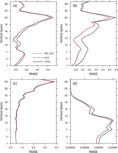
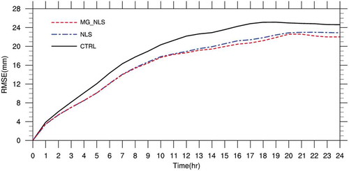
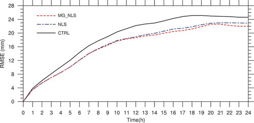
Figure 2. RMSEs of the 24-h forecast of accumulated rainfall (from 0000 UTC 8 August to 0000 UTC 9 August) with the initial condition from CTRL, nonlinear least squares (NLS) assimilation with $I_{max}=3$, and multigrid NLS (MG_NLS) with $n=3$ methods.

To evaluate their efficiency, we compared the central processing unit (CPU) times of NLS with $I_{max}=3$ and MG_NLS with $n=3$. The experiments were implemented serially using a Dell PowerEdge R610 server at 24-GB memory and 2.40 GHz with 16 CPUs (16 × 4 [2-thread] Intel Xeon CPU E5620). The forecast model ran on 24 cores in parallel. It is important to note that the CPU time for model implementation depended on the case and the given CPU. The CPU times for MG_NLS with $n=3$ and NLS with $I_{max}=3$ is different. A forecast model was run for each iteration. The CPU time for NLS was the sum of 909.520 s and 120 s, where the former is the time of the assimilation process and the latter is twice the time of the forecast model operation. The CPU time for MG_NLS was 481.459 s for the assimilation process, which was almost half that of the NLS method. Therefore, the computational cost was reduced by the multigrid strategy.

To further investigate the effect of the number of total grid levels $\mathrm{n}$ on multi-scale error in the assimilation, we compared the performances when using different total numbers of grid levels for MG_NLS (referred to as MG_NLS_i, $i=2,3$, where $i$ represents the total number of grid levels). MG_NLS₂ represents two grid levels (130 × 110 and 260 × 220), and MG_NLS₃ is the same as MG_NLS with $n=3$ referred to earlier. 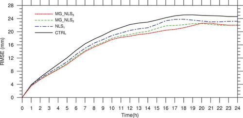For comparison, NLS₁ (with one grid level; 260 × 220 grid points) is the same as NLS with $I_{max}=3$ referred to earlier. The RMSEs of the 24-h forecast of accumulated rainfall with CTRL and the three schemes, NLS₁ and MG_NLS_i, had smaller RMSEs than CTRL (Figure 3), indicating that the three methods assimilated the observations correctly, creating a more accurate rainfall forecast. The forecast accuracy increased gradually with the number of total grid levels. MG-NLS₃ outperformed MG-NLS₂ and NLS₁; thus, the three grid levels more effectively accounted for and minimized background error, starting from large-scale error and working towards error at a small scale, for a more accurate analysis.

Figure 3. RMSEs of 24-h forecast of accumulated rainfall (from 0000 UTC 8 August to 0000 UTC 9 August) with the initial condition from the CTRL, nonlinear least squares (NLS₁), and multigrid NLS (MG_NLS_i) ($\mathrm{i}=2,3$ represents the total number of grid levels) methods.

The total times for the NLS₁, MG_NLS, and MG_NLS₃ methods were 300.368, 483.958, and 601.459 s, respectively (Table 1). The computational cost increased with the number of horizontal grids. The time for the forecast model operation to run once was about 60 s. Although MG-NLS₃ had the highest computational cost, its higher forecast accuracy was worth the extra but almost negligible computational cost. Moreover, compared with NLS with $I_{max}=3$ referred to earlier, which is slightly lower accuracy, MG-NLS₃ had greatly improved computing efficiency.

Table 1. CPU time of each grid level and total time for NLS₁ and MG_NLS_i ($i=2,3$, where $\mathrm{i}$ represents the number of grid levels) (units: s).

Method	NLS1	MG_NLS2	MG_NLS3
65 × 55	0	0	62.729 + 60
130 × 110	0	118.916 + 60	112.735 + 60
260 × 220	300.368	305.041	305.994
Total time (s)	300.368	483.958	601.459

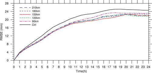
To test the sensitivity of MG_NLS with $n=3$, the RMSEs of the 24-h forecast of accumulated rainfall of MG_NLS with five localization radii were compared (Figure 4). The RMSE was smallest when the localization radius was 150 km. Therefore, this radius was used for MG_NLS and NLS in the OSSEs. The MG_NLS performance was similar when the localization radius varied from 120 to 210 km, indicating that MG_NLS has low sensitivity to the localization radius of the interval.

Figure 4. RMSEs of the 24-h forecast of accumulated rainfall (from 0000 UTC 8 August to 0000 UTC 9 August) with the initial condition from CTRL and multigrid nonlinear least-squares assimilation (MG_NLS) ($n=3$) with different localization radii.

4. Conclusions

Ensemble-based variational data assimilation methods have flow-dependent background error covariance matrices $\text{bi}B$ and avoid the adjoint model; however, their accuracy depends on iterative corrections on a given scale. The assimilation of unconventionally observed radar data using a large number of observations and high time frequency incurs a high computational cost. The MG_NLS-4DVar method used in this paper not only has the advantages of ensemble-based variational data assimilation, but also corrects the background error from large to small scales. Ultimately, the analysis field is the sum of the background field and the analysis increment on all grid levels. In this paper, a triple-grid MG_NLS-4DVar method was used to assimilate the radar radial velocity of Ningbo station to assess the capabilities of MG_NLS-4DVar. The main conclusions can be summarized as follows.

Both NLS-4DVar and MG_NLS-4DVar can effectively assimilate radar radial velocity to improve the initial field and enhance the 24-h cumulative precipitation forecast accuracy. Also, MG_NLS-4DVar outperforms NLS-4DVar. In terms of assimilation CPU time, the computational cost of NLS-4DVar with three iterations on the finest grid was found to be higher. The precision of MG_NLS-4DVar improved as the total number of grids increased. Therefore, the MG_NLS-4DVar method, with dual advantages in assimilation accuracy and computational efficiency, is a promising tool for radar radial velocity data assimilation. Only a limited area was covered in this paper because the radar radial velocity observations were from a single radar. Multiple radar observations and the radar reflectivity are expected to be assimilated with MG_NLS-4DVar in the future.

Acknowledgments

We thank Dr. FENG Chen at the Zhejiang Institute of Meteorological Sciences for providing the radar data and helpful comments and suggestions, and Dr. ZHANG Bin for data analysis. We thank NCAR, Boulder, Colorado, USA, for making the WRF-ARW model available (http://www2.mmm.ucar.edu/wrf/users/downloads.html). The initial and lateral boundary conditions are generated by NCEP FNL operational global analysis data (https://rda.ucar.edu/datasets/ds083.2/).

Disclosure statement

No potential conflict of interest was reported by the authors.

Additional information

Funding

The work was partially supported by the National Key Research and Development Program of China [grant number 2016YFA0600203]; the National Natural Science Foundation of China [grant number 41575100]; and the Key Research Program of Frontier Sciences, Chinese Academy of Sciences [grant number QYZDY-SSW-DQC012].

References

- Bao, X., Y. Luo, J. Sun, Z. Meng, and J. Yue. 2017. “Assimilating Doppler Radar Observations with an Ensemble Kalman Filter for Convection Permitting Prediction of Convective Development in a Heavy Rainfall Event during the Pre-summer Rainy Season of South China.” Science China Earth Sciences 60: 1866. doi:10.1007/s11430-017-9076-9.
- Fabry, F., and A. Kilambi. 2011. “The Devil Is in the Details: Preparing Radar Information for Its Proper Assimilation.” 35th Conf. on Radar Meteorology, Pittsburgh, PA, Amer. Meteor. Soc., 19A.6. https://ams.confex.com/ams/35Radar/webprogram/Paper191698.html
- Fu, H., X. R. Wu, W. Li, Y. F. Xie, G. J. Han, and S. Q. Zhang. 2016. “Reconstruction of Typhoon Structure Using 3-dimensional Doppler Radar Radial Velocity Data with the Multigrid Analysis: A Case Study in an Idealized Simulation Context.” Advances in Meteorology 2016: 1–10. doi:10.1155/2016/2170746.
- Ide, K., P. Courtier, M. Ghil, and A. C. Lorenc. 1997. “Unified Notation for Data Assimilation: Operational, Sequential and Variational.” Journal of the Meteorological Society of Japan 75 (1B): 181–189. doi:10.2151/jmsj1965.75.1B_181.
- Kalnay, E., and S. C. Yang. 2010. “Accelerating the Spin-up of Ensemble Kalman Filtering.” Quarterly Journal of the Royal Meteorological Society 136 (651): 1644–1651. doi:10.1002/qj.652.
- Li, W., Y. Xie, S. Deng, and Q. Wang. 2010. “Application of the Multigrid Method to the Two-Dimensional Doppler Radar Radial Velocity Data Assimilation.” The Journal of Atmospheric and Oceanic Technology 27: 319–332. doi:10.1175/2009JTECHA1271.1.
- Lorenc, A. C. 2003. “The Potential of the Ensemble Kalman Flter for NWP—Acomparison with 4d-var.” Quarterly Journal of the Royal Meteorological Society 129: 3183–3203. doi:10.1256/qj.02.132.
- Sun, J., and N. A. Crook. 1997. “Dynamical and Microphysical Retrieval from Doppler Radar Observations Using a Cloud Model and Its Adjoint: Part I. Model Development and Simulated Data Experiments.” Journal of the Atmospheric Sciences 54: 1642–1661. doi:10.1175/1520-0469(1997)054<1642:DAMRFD>2.0.CO;2.
- Sun, J., and N. A. Crook. 1998. “Dynamical and Microphysical Retrieval from Doppler Radar Observations Using a Cloud Model and Its Adjoint: Part II. Retrieval Experiments of an Observed Florida Convective Storm.” Journal of the Atmospheric Sciences 55: 835–852. doi:10.1175/1520-0469(1998)055<0835:DAMRFD>2.0.CO;2.
- Sun, J., and H. Wang. 2013. “Radar Data Assimilation with WRF 4d-var. Part II: Comparison with 3d-var for a Squall Line over the U.S. Great Plains.” Monthly Weather Review 141: 2245–2264.
- Thompson, T. E., L. J. Wicker, and X. Wang. 2012. “Impact from a Volumetric Radar-sampling Operator for Radial Velocity Observations within EnKF Supercell Assimilation.” The Journal of Atmospheric and Oceanic Technology 29: 1417–1427. doi:10.1175/JTECH-D-12-00088.1.
- Tian, X. J., and X. B. Feng. 2015. “A Non-linear Least Squares Enhanced POD-4DVar Algorithm for Data Assimilation.” Tellus A 67: 25340. doi:10.3402/tellusa.v67.25340.
- Tian, X. J., Z. H. Xie, and A. G. Dai. 2008. “An Ensemble-based Explicit Four-dimensional Variational Assimilation Method.” Journal of Geophysical Research 113: D21124. doi:10.1029/2008JD010358.
- Tian, X. J., Z. H. Xie, and Q. Sun. 2011. “A POD-based Ensemble Four-dimensional Variational Assimilation Method.” Tellus A 63: 805–816. doi:10.1111/j.1600-0870.2011.00529.x.
- Tian, X. J., H. Q. Zhang, X. B. Feng, and Y. F. Xie. 2018. “Nonlinear Least Squares En4DVar to 4denvar Methods for Data Assimilation: Formulation, Analysis and Preliminary Evaluation.” Monthly Weather Review 146: 77–93. doi:10.1175/MWR-D-17-0050.1.
- Wang, H., J. Sun, X. Zhang, X. Huang, and T. Auligne´. 2013. “Radar Data Assimilation with WRF 4d-var. Part I: System Development and Preliminary Testing.” Monthly Weather Review 141: 2224–2244. doi:10.1175/MWR-D-12-00168.1.
- Xie, Y., S. Koch, J. McGinley, S. Albers, P. E. Bieringer, M. Wolfson, and M. Chan. 2011. “A Space–Time Multiscale Analysis System: A Sequential Variational Analysis Approach.” Monthly Weather Review 139 (4): 1224–1240. doi:10.1175/2010MWR3338.1.
- Xie, Y., S. E. Koch, J. A. McGinley, S. Albers, and N. Wang. 2005. “A Sequential Variational Analysis Approach for Mesoscale Data Assimilation, Preprints.” 21st Conf. on Weather Analysis and Forecasting/17th Conf. on Numerical Weather Prediction, Washington, DC: Amer. Meteor. Soc., 15B.7. http://ams.confex.com/ams/pdfpapers/93468.pdf.
- Zhang, B., X. Tian, J. Sun, F. Chen, Y. Zhang, L. Zhang, and S. Fu. 2015. “PODEn4DVar-based Radar Data Assimilation Scheme: Formulation and Preliminary Results from Real-data Experiments with Advanced Research WRF(ARW).” Tellus A 67: 26045. doi:10.3402/tellusa.v67.26045.
- Zhang, B., X. J. Tian, L. F. Zhang, and J. H. Sun. 2017a. “The Radar Data Assimilation System Based on NLS-4DVar and Its Application. in Heavy Rain Forecast.” Chinese Journal of Atmospheric Sciences (in Chinese) 41 (2): 321−332. doi:10.3878/j.issn.1006-9895.1607.16103.
- Zhang, H., J. Xue, S. Zhuang, G. Zhu, and Z. Zhu. 2004. “GRAPeS 3d-var Data Assimilation System Ideal Experiments.” Acta Meteorologica Sinca 62: 31–41.
- Zhang, H. Q., and X. J. Tian. 2018a. “A Multigrid NLS-4DVar Data Assimilation Scheme with Advanced Research WRF (ARW).” Journal of Geophysical Research 123: 5116–5129. doi:10.1029/2017JD027529.
- Zhang, H. Q., and X. J. Tian. 2018b. “An Efficient Local Correlation Matrix Decomposition Approach for the Localization Implementation of Ensemble-based Assimilation Methods.” Journal of Geophysical Research: Atmospheres 123. doi:10.1002/2017JD027999.
- Zhang, L., X. J. Tian, X. F. Liu, and C. X. Shi. 2017b. “NLS-3DVar Data Fusion Method Based on Multigrid Implementation Strategy and Its Application in Temperature Data Fusion.” Climatic and Environmental Research (in Chinese) 22 (3): 271–288. doi:10.3878/j.issn.1006-9585.2016.16140.