Subseasonal variabilities of surface soil moisture in reanalysis datasets and CESM simulations

ABSTRACT

Using surface soil moisture (SM) from ERA-Interim reanalysis and Climate Forecast System Reanalysis (CFSR) data together with simulated results from CESM, the authors evaluated the subseasonal variability of SM and explored its basic features. Evident subseasonal variability of SM was detected in all seasons and with different datasets. However, the subseasonal variability of SM showed significant regional differences and varied with seasons. It was found that SM has large subseasonal variances in eastern China, North America, South Africa, and Australia in the summer hemisphere. The variances of the low-frequency SM variations given by ERA-Interim and CFSR are different. Overall, CFSR shows stronger variability than ERA-Interim. Through spectral analysis, it was noticed that low-frequency variations of surface SM mainly happen with periods of 10–30 days and 30–50 days. Subseasonal variations with a period of 10–30 days are dominant in eastern China and South Africa. However, subseasonal variations with periods of both 10–30 days and 30–50 days were detected in North America and Australia. Generally, CESM captures the main features of SM subseasonal variation. However, the model overestimates the subseasonal variability in all seasons in most regions, especially in the high latitudes of the Northern Hemisphere.

Graphical abstract

摘要

利用欧洲中心(ERA-Interim)和美国气候预测系统（CFSR）再分析资料，结合地球系统模式CESM的模拟结果，考察了1979–2016年全球表层土壤湿度次季节变率的基本特征。在各个季节和所有资料中，土壤湿度均有明显的次季节变率，且有明显的区域和季节性差异。在中国东部、北美、南非、澳大利亚的夏季，土壤湿度有较大的次季节方差，CFSR和CESM中的土壤湿度变率强于ERA-Interim。通过谱分析，发现中国东部和南非的土壤湿度主要为10–30天的周期，北美和澳大利亚的土壤湿度同时具有10–30天和30–50天的周期。

KEYWORDS:

• Soil moisture
• subseasonal variability
• land–atmosphere interaction

关键词:

• 土壤湿度；次季节变率；陆–气相互作用

1. Introduction

Soil moisture (SM) plays a key role in the climate system, being an important impact factor for hydrology, ecology, and meteorology (Jipp et al. 1998; Legates et al. 2011; Manzoni, Schimel, and Porporato 2012; Jia et al. 2017; Chou et al. 2018). SM can directly affect land-surface evaporation and terrestrial vegetation activity, and further adjust water and energy balances at the land surface (Ying et al. 2016; Alavi et al. 2016). Because of the soil water content, soil can keep abnormal signals for a longer time than the atmosphere (Koster and Suarez 2000), which is usually referred to as the ‘memory’ of SM (Seneviratne et al. 2006). Meanwhile, anomalous SM has important impacts on land-surface conditions, near-surface meteorological elements, and even atmospheric general circulation (e.g. Manabe 1969; Berg et al. 2017; Huang and Margulis 2013). Therefore, investigation into the variability of SM is necessary to better our understanding of land–atmosphere interaction and its associated mechanisms.

The spatiotemporal variations of SM have been widely investigated (Entin et al. 2000; Cheng et al. 2015; Huang et al. 2016). Previous studies have indicated that SM usually shows an evident seasonal cycle, which is closely related to the seasonality of precipitation (Nie, Luo, and Zhu 2008; Berg et al. 2017). In addition, large interannual variabilities of SM are found in central North America, Europe, and West Asia (Yang, Wang, and Bao 2016). On decadal and longer time scales, SM shows evident wetting (drying) trends in most arid and humid (semiarid) regions (Ma, Wei, and Fu 2000; Li, Ma, and Niu 2011; Zhang and Zuo 2011). Huang et al. (2016) pointed out that the area of drylands has expanded significantly over semi-arid regions since the early 1960s. Regarding the spatial distribution of global SM, the largest SM occurs in the tropics, eastern North America, and from northern Europe to Russia; and the smallest SM can be found in deserts and semi-arid areas (Mccoll et al. 2017). Notably, the variabilities of SM on various time scales exhibit evident regional differences.

Many studies have pointed out that SM variation is important for the variabilities of the atmosphere on various time scales. For example, in Australia, extreme heatwaves are strongly related to the leading dry soil condition (Perkins, Argüeso, and White 2015). On seasonal and interannual time scales, persistent SM anomalies can cause significant impacts on precipitation (Liu, Zhang, and Zuo 2017). It has also been found that, by including realistic SM with interannual variation, models can produce more reasonable precipitation in the East Asian summer monsoon region (Li et al. 2015). On the intraseasonal time scale, Saha, Pokhrel, and Chaudhari (2013) found that the intraseasonal variation of the Indian summer monsoon is significantly associated with the intraseasonal variation of SM. Also, the subseasonal variability of the West African monsoon is also closely linked to the subseasonal variation of SM (Taylor 2008). Furthermore, SM variability is considered a key factor in the dominant modes of the intraseasonal variability of monsoon activity (Taylor 2008; Lavender, Taylor, and Matthews 2010). In addition, the initialization of SM can greatly improve the skill of subseasonal to seasonal climate predictions (Koster et al. 2009; Seo et al. 2018).

Even though the seasonal and interannual variability of SM has been widely explored, the subseasonal variations of SM are still not clear in both observations and model simulations. This paper attempts to reveal the subseasonal variability of SM based on reanalysis and model simulation data. Section 2 describes the data used. In section 3, the subseasonal variations of SM and their spectral features are investigated. Section 4 briefly summarizes our main findings.

2. Data and methods

2.1 Data

The 6-h SM data from the ERA-Interim and Climate Forecast System Reanalysis (CFSR) datasets during 1979–2016 were used in this study. The ERA-Interim data were obtained from the website of the European Centre for Medium-Range Weather Forecasts (https://www.ecmwf.int). The CFSR data can be acquired from the Research Data Archive of the US National Center for Atmospheric Research (https://rda.ucar.edu). Surface SM data (in m³ m⁻³) were selected at the depths of 0–7 cm and 0–10 cm from ERA-Interim and CFSR, respectively. The horizontal resolution of the ERA-Interim SM data is 1.5° × 1.5°, and the CFSR SM data are on 192 × 92 Gaussian grids. The original resolutions of both datasets were used in our analysis and the 6-h data were averaged into daily means.

In addition, the simulation results during 1985–2013 from the interactive atmosphere and land coupled mode of the Community Earth System Model, version 1.2.2 (CESM), with observational forcing, were used. The simulated SM given by the model is at daily intervals, at the depth of 0–9.1 cm, and on 192 × 288 Gaussian grids. The land surface model in CESM is the Community Land Model, version 4.0. The configurations of the model were similar to those in Wei et al. (2014). Note that ERA-Interim and CFSR were examined during the same period of 1979–2016, while the time period used for CESM was 1985–2013. We also analyzed the results during 1985–2013 for all three datasets, and obtained similar conclusions. In order to prove that the SM subseasonal variability widely exists in most years, the entire time period of each dataset was examined.

2.2 Methods

A 10–90-day bandpass filter was used to obtain the subseasonal component of the variation in daily SM (Duchon 1979). The four seasons were defined as March–May (spring), June–August (summer), September–November (autumn), and December–February (winter). Note that, in our study, the four seasons were defined according to those of the Northern Hemisphere. During the bandpass filtering, the data were extended forwards and backwards by 1 month, and then the data in each season were picked out for analysis. The standard deviation in each season was used to represent the subseasonal variability of SM.

3. Results

3.1 Subseasonal variability of surface SM

Figure 1 presents the geographic distribution of the subseasonal variability of the surface SM defined by seasonally averaged variances of 10–90-day bandpass-filtered daily SM from the ERA-Interim and CFSR data. The variability of SM examined in this study is mainly on the subseasonal time scale of 10–90 days. SM exhibits evident subseasonal variabilities in both datasets, characterized by significant regional differences and distinct seasonality. Overall, the spatial patterns of the subseasonal variability estimated from the two datasets are consistent, but CFSR gives a stronger subseasonal signal, covering a more extensive land area, than ERA-Interim.

Figure 1. Subseasonal variances of surface soil moisture (SM) in spring (top row), summer (second row), autumn (third row), and winter (bottom panels), calculated using (a–d) ERA-Interim, (e–h) CFSR, and (i–l) CESM. Subseasonal variance is defined as the standard deviation of SM that is bandpass-filtered by the cut-off of 10–90 days. During the filtering, the time period of the data was extended forwards and backwards by 1 month, and then the data in spring, summer, autumn, and winter were picked out to calculate the standard deviations. The reanalysis data (ERA-Interim and CFSR) covered the period 1979–2016, while the results of CESM covered 1985–2013. The rectangles surround areas with large variances in summer (b, f, and j) and winter (d, h, and l) over the Northern and Southern Hemisphere.

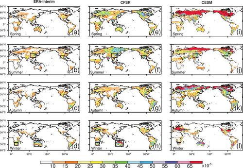
In spring (Figure 1(a,e)), evident subseasonal variabilities mainly appear in East Europe, East Asia, and North America in the Northern Hemisphere, but in East and South Africa, Australia, Argentina, and Brazil in the Southern Hemisphere. In summer (Figure 1(b,f)), large variances are mainly located in the Northern Hemisphere, especially over India, eastern China, and North America. In autumn (Figure 1(c,g)), the distributions of SM variances are similar to those in spring, but weaker. In winter (Figure 1(d,h)), large SM variances are generally found over South Africa, Australia, and the southern part of South America. We also evaluated the subseasonal variations of SM in the deep soil layer (100–200 cm) (figure not shown), and similar spatial patterns of SM subseasonal variabilities were found. However, the variabilities of SM in the deep soil layer were much weaker than those of the surface layer, which could be related to the relatively weak impact of atmospheric forcing on soil water in the deep soil layer.

We also evaluated the subseasonal variability simulated by CESM (Figure 1(i–l)). Generally, CESM can capture the main features of the subseasonal variation of SM, in terms of both the spatial pattern and the period of the low-frequency variation of SM. However, the model overestimates the subseasonal variability of SM in all seasons in most regions of the global land area, especially in the high latitudes of the Northern Hemisphere. The overestimation of the subseasonal variability of SM might be related to the rainfall bias and misinterpretation of land processes in the model, which deserves further investigation.

3.2 Spectral features of SM

To further investigate the spectral features of SM, several target areas with significant subseasonal variability, as marked by the rectangles in Figure 1, were chosen and the regionally averaged SM over the target regions calculated.

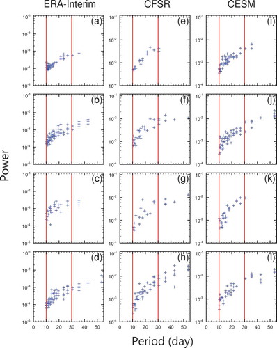
Figure 2 shows significant spectral peaks of 10–90 days in each year during 1979–2016 (1985–2013) for ERA-Interim and CFSR (CESM). Those peaks were calculated during each season of each year by using the fast Fourier transform method, and were found to be significant at the 0.05 level according to the Markov red noise test. In each season, data were extended forwards and backwards by 1 month. Because most of the significant spectral peaks are between 10 and 50 days, the x-axis in Figure 2 is only drawn from 0 to 50 days. Moreover, significant peaks during 0–10 days are not plotted. From Figure 2, in both summer hemispheres, there are significant spectral peaks on the subseasonal time scale. Most of the spectra are between 10 and 30 days. In eastern China (Figure 2(a,e,i)), summer spectral peaks are mainly between 10 and 30 days. In North America (Figure 2(b,f,g)), summer spectral peaks are also found between 30 and 50 days. In South Africa (Figure 2(c,g,k)), winter spectral peaks are also mainly between 10 and 30 days, but less frequent than those in the Northern Hemisphere. In Australia (Figure 2(d,h,l)), there are also winter spectral peaks between 30 and 50 days, similar to those in North America, but the number of spectral peaks is evidently smaller than that in North America. Overall, there are significant spectral peaks between 10 and 30 days in the Southern Hemisphere, but the number of spectral peaks is larger in the Northern Hemisphere than in the Southern Hemisphere. There are also spectral peaks between 30 and 50 days in North America and Australia.

Figure 2. Significant spectral peaks during 10–90 days (x-axis) in each year of 1979–2016 for ERA-Interim and CFSR, and of 1985–2013 for CESM. Spectra were obtained using the fast Fourier transform method. The Markov red noise test was used for significance testing, revealing the peaks to be significant at the 0.05 level. Panels in the top two rows are for areas in the Northern Hemisphere in summer. Panels (a, e, i) are for eastern China, and (b, f, j) are for North America. Panels in the bottom two rows are for areas in the Southern Hemisphere in winter. Panels (c, g, k) are for South Africa, and (d, h, l) are for Australia. Panels (a–d) are for ERA-Interim, (e–h) are for CFSR, and (i–l) are for CESM. The two red reference lines are at 30 and 60 days, respectively.

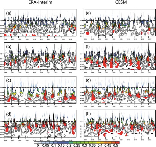
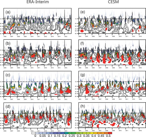
The variation of the spectral features with time was also checked, through wavelet analysis (Figure 3). The wavelet spectra of the original daily SM are presented for ERA-Interim during 1979–2015 and for CESM during 2004–13. Only the aforementioned spectra during 2004–13 are shown, because the results for CFSR are similar to those shown in Figure 3. In Figure 3(a,e), the spectra on subseasonal time scales are generally significant at 10–30 days in eastern China. In North America (Figure 3(b,f)), significant spectra are found between 10 and 30 days and between 30 and 50 days. In South Africa (Figure 3(c,g)), the distribution of spectra is quite similar to that in North America, but the significant areas are smaller than those in the Northern Hemisphere. In Australia (Figure 3(d,h)), more significant spectra are found than in South Africa, and mainly at 10–30 days and 30–50 days. It is interesting that the 10–30-day spectra occur throughout the seasons in both hemispheres, but the 30–50-day spectra mostly happen at the start and end of each season.

Figure 3. Wavelet analysis for soil moisture in ERA-Interim during 2006–2015 (a–d) and CESM during 2004–13 (e–h). Panels in the top (bottom) two rows correspond to the two areas in the Northern (Southern) Hemisphere in summer, similar to those shown in Figure 2. Significant spectra are shaded, having been tested against Markov red noise.

4. Summary and discussion

Using surface SM data from ERA-Interim and CFSR together with simulated results from CESM, we evaluated the subseasonal variability of SM and explored the basic features of the subseasonal variation of SM.

Results showed that evident subseasonal variability of SM can be detected in all seasons and with different datasets. However, the subseasonal variability of SM shows significant regional differences and varies with season. It was found that SM has large subseasonal variances over eastern China, North America, South Africa, and Australia in the summer hemisphere. The variances of the low-frequency SM variation given by ERA-Interim and CFSR are different. Overall, CFSR shows stronger variability than ERA-Interim. Through spectral analysis, it was found that the low-frequency variations of surface SM mainly happen with periods of 10–30 days and 30–50 days. The subseasonal variations with a period of 10–30 days are dominant in eastern China and South Africa. However, subseasonal variations with periods of both 10–30 days and 30–50 days can be detected in North America and Australia. Generally, CESM can capture the main features of the subseasonal variation of SM, in terms of both the spatial pattern and the period of the low-frequency variation in SM. However, CESM overestimates the subseasonal variability of SM in all seasons in most regions of the global land area, especially in the high latitudes of the Northern Hemisphere.

This paper presents some preliminary results on the subseasonal variability of SM. However, owing to the limitations of the SM data used, a detailed evaluation of the subseasonal variability is still necessary in the future. In addition, the subseasonal variabilities of other land-surface variables, together with their possible causes and potential impacts, deserve further investigation. We also noticed that the model shows limited capability in capturing the subseasonal variability of SM. Thus, it is also necessary to improve the model’s performance in simulating the subseasonal variability of land-surface variables and their relevant processes, which will be helpful towards improving the subseasonal-to-seasonal prediction skill of numerical models. It is interesting that the memory of SM mainly operates on the subseasonal time scale (Seneviratne et al. 2006), and SM has significant subseasonal variability on such a time scale. The possible link between the subseasonal variability of SM and its memory deserves further study, which will help to better understand the nature of the subseasonal variability of SM.

Disclosure statement

No potential conflict of interest was reported by the authors.

Additional information

Funding

This study was supported by the National Natural Science Foundation of China [grant number 41625019].

References

- Alavi, N., S. Bélair, V. Fortin, S. L. Zhang, S. Z. Husain, M. L. Carrera, and M. Abrahamowicz. 2016. “Warm Season Evaluation of Soil Moisture Prediction in the Soil, Vegetation, and Snow (SVS) Scheme.” Journal of Hydrometeorology 17 (8): 2315–2332. doi:10.1175/jhm-d-15-0189.1.
- Berg, A., B. Lintner, K. Findell, and A. Giannini. 2017. “Soil Moisture Influence on Seasonality and Large-Scale Circulation in Simulations of the West African Monsoon.” Journal of Climate 30 (7): 2295–2317. doi:10.1175/JCLI-D-15-0877.1.
- Cheng, S., X. Guan, J. Huang, F. Ji, and R. Guo. 2015. “Long-Term Trend and Variability of Soil Moisture over East Asia.” Journal of Geophysical Research-Atmospheres 120 (17): 8658–8670. doi:10.1002/2015JD023206.
- Chou, C., D. Ryu, M. H. Lo, H. W. Wey, and H. M. Malano. 2018. “Irrigation Induced Land-Atmosphere Feedback and Their Impacts on Indian Summer Monsoon.” Journal of Climate 31 (21): 8785–8801. doi:10.1175/jcli-d-17-0762.1.
- Duchon, C. E. 1979. “Lanczos Filtering in One and Two Dimensions.” Journal of applied meteorology 18 (8): 1016–1022. doi:10.1175/1520-0450(1979)018<1016:LFIOAT>2.0.CO;2.
- Entin, J. K., A. Robock, K. Y. Vinnikov, S. E. Hollinger, S. Liu, and A. Namkhai. 2000. “Temporal and Spatial Scales of Observed Soil Moisture Variations in the Extratropics.” Journal of Geophysical Research Atmospheres 105 (D9): 11865–11877. doi:10.1029/2000jd900051.
- Huang, H. Y., and S. A. Margulis. 2013. “Impact of Soil Moisture Heterogeneity Length Scale and Gradients on Daytime Coupled Land-Cloudy Boundary Layer Interactions.” Hydrological Processes 27 (14): 1988–2003. doi:10.1002/hyp.9351.
- Huang, J., M. Ji, Y. Xie, S. Wang, Y. He, and J. Ran. 2016. “Global Semi-Arid Climate Change over Last 60 Years.” Climate Dynamics 46 (3–4): 1131–1150. doi:10.1007/s00382-015-2636-8.
- Jia, X., M. Shao, Y. Zhu, and Y. Luo. 2017. “Soil Moisture Decline Due to Afforestation across the Loess Plateau, China.” Journal of Hydrology 546: 113–122. doi:10.1016/j.jhydrol.2017.01.011.
- Jipp, P. H., D. C. Nepstad, D. K. Cassel, and C. R. D. Carvalho. 1998. “Deep Soil Moisture Storage and Transpiration in Forests and Pastures of Seasonally-Dry Amazonia.” Climatic Change 39 (2–3): 395–412. doi:10.1023/a:1005308930871.
- Koster, R. D., Z. C. Guo, P. A. Dirmeyer, R. Q. Yang, K. Mitchell, and M. J. Puma. 2009. “On the Nature of Soil Moisture in Land Surface Models.” Journal of Climate 22 (22): 4322–4335. doi:10.1175/2009jcli2832.1.
- Koster, R. D., and M. J. Suarez. 2000. “Soil Moisture Memory in Climate Models.” Journal of Hydrometeorology 2 (6): 558–570. doi:10.1175/1525-7541(2001)0022.0.CO;2.
- Lavender, S. L., C. M. Taylor, and A. J. Matthews. 2010. “Coupled Land-Atmosphere Intraseasonal Variability of the West African Monsoon in a GCM.” Journal of Climate 23 (21): 5557–5571. doi:10.1175/2010JCLI3419.1.
- Legates, D. R., R. Mahmood, D. F. Levia, T. L. DeLiberty, S. M. Quiring, C. Houser, and F. E. Nelson. 2011. “Soil Moisture: A Central and Unifying Theme in Physical Geography.” Progress in Physical Geography 35 (1): 65–86. doi:10.1177/0309133310386514.
- Li, M. X., Z. G. Ma, and G. Y. Niu. 2011. “Modeling Spatial and Temporal Variations in Soil Moisture in China.” Chinese Science Bulletin (in Chinese) 56 (17): 1809–1820. doi:10.1007/s11434-011-4493-0.
- Li, Z., T. Zhou, H. Chen, D. Ni, and R.-H. Zhang. 2015. “Modelling the Effect of Soil Moisture Variability on Summer Precipitation Variability over East Asia.” International Journal of Climatology 35 (6): 879–887. doi:10.1002/joc.4023.
- Liu, L., R. Zhang, and Z. Zuo. 2017. “Effect of Spring Precipitation on Summer Precipitation in Eastern China: Role of Soil Moisture.” Journal of Climate 30 (20): 9183–9194. doi:10.1175/JCLI-D-17-0028.1.
- Ma, Z. G., H. L. Wei, and C. B. Fu. 2000. “Relationship between Regional Soil Moisture Variation and Climatic Variability over East China.” Acta Meteorologica Sinica (in Chinese) 58 (3): 278–287.
- Manabe, S. 1969. “Climate and the Ocean Circulation 1. The Atmospheric Circulation and the Hydrology of the Earth’s Surface.” Monthly Weather Reviewer 97 (1): 739–774. doi:10.1175/1520-0493(1969)097<0739:CATOC>2.3.CO;2.
- Manzoni, S., J. P. Schimel, and A. Porporato. 2012. “Responses of Soil Microbial Communities to Water Stress: Results from A Meta-Analysis.” Ecology 93 (4): 930–938. doi:10.1890/11-0026.1.
- Mccoll, K. A., S. H. Alemohammad, R. Akbar, A. G. Konings, S. Yueh, and D. Entekhabi. 2017. “The Global Distribution and Dynamics of Surface Soil Moisture.” Nature Geoscience 10 (2): 100–104. doi:10.1038/ngeo2868.
- Nie, S., Y. Luo, and J. Zhu. 2008. “Trends and Scales of Observed Soil Moisture Variations in China.” Advances in Atmospheric Sciences 25 (1): 43–58. doi:10.1007/s00376-008-0043-3.
- Perkins, S. E., D. Argüeso, and C. J. White. 2015. “Relationships between Climate Variability, Soil Moisture, and Australian Heatwaves.” Journal of Geophysical Research: Atmospheres 120 (16): 8144–8164. doi:10.1002/2015JD023592.
- Saha, S. K., S. Pokhrel, and H. S. Chaudhari. 2013. “Influence of Eurasian Snow on Indian Summer Monsoon in NCEP CFSv2 Freerun.” Climate Dynamics 41 (7–8): 1801–1815. doi:10.1007/s00382-012-1617-4.
- Seneviratne, S. I., R. D. Koster, Z. Guo, P. A. Dirmeyer, E. Kowalczyk, D. Lawrence, P. Liu, et al. 2006. “Soil Moisture Memory in AGCM Simulations: Analysis of Global Land–Atmosphere Coupling Experiment (GLACE) Data.” Journal of Hydrometeorology 7 (5): 1090–1112. doi:10.1175/jhm533.1.
- Seo, E., M. I. Lee, J. H. Jeong, R. D. Koster, S. D. Schubert, H. M. Kim, D. Kim, et al. 2018. “Impact of Soil Moisture Initialization on Boreal Summer Subseasonal Forecasts: Mid-Latitude Surface Air Temperature and Heat Wave Events.” Climate Dynamics 52 (3–4): 1–15. doi:10.1007/s00382-018-4221-4.
- Taylor, C. M. 2008. “Intraseasonal Land-Atmosphere Coupling in the West African Monsoon.” Journal of Climate 21 (24): 6636–6648. doi:10.1175/2008jcli2475.1.
- Wei, N., Y. Dai, M. Zhang, L. Zhou, D. Ji, S. Zhu, and L. Wang. 2014. “Impact of Precipitation‐induced Sensible Heat on the Simulation of Land‐surface Air Temperature.” Journal of Advances in Modeling Earth Systems 6 (4): 1311–1320. doi: 10.1002/2014MS000322.
- Yang, K., C. Wang, and H. Bao. 2016. “Contribution of Soil Moisture Variability to Summer Precipitation in the Northern Hemisphere.” Journal of Geophysical Research-Atmospheres 121 (20): 12108–12124. doi:10.1002/2016JD025644.
- Ying, K., T. Zhao, X. Zheng, X. W. Quan, C. S. Frederiksen, and M. Li. 2016. “Predictable Signals in Seasonal Mean Soil Moisture Simulated with Observation-Based Atmospheric Forcing over China.” Climate Dynamics 47 (7–8): 2373–2395. doi:10.1007/s00382-015-2969-3.
- Zhang, R., and Z. Zuo. 2011. “Impact of Spring Soil Moisture on Surface Energy Balance and Summer Monsoon Circulation over East Asia and Precipitation in East China.” Journal of Climate 24 (13): 3309–3322. doi:10.1175/2011JCLI4084.1.