Contributions of climate change, land use change and CO₂ to changes in the gross primary productivity of the Tibetan Plateau

ABSTRACT

The ecosystems on the Tibetan Plateau (TP) are highly vulnerable to climate change, rising CO₂ concentration, and land-use and land-cover change (LULCC), but their contributions to changes in the gross primary productivity (GPP) of the TP are not clearly understood. In this study, the role of these three factors on the interannual variations (IAVs) and trends of the TP’s GPP were investigated using 12 terrestrial biosphere models. The ensemble simulations showed that climate change can explain most of the changes in the GPP, while the direct effect of LULCC and rising CO₂ (mainly fertilization effect) contributed 10% and −14% to the mean GPP values, 37% and −20% to the IAV, and 52% and −24% to the GPP’s trend, respectively. The LULCC showed higher contributions to the significant positive trend in the annual GPP of the TP. However, the results from different model simulations showed that considerable uncertainties were associated with the effects of LULCC on the GPP of the TP.

Key figure (only for online)

摘要

青藏高原（TP）的生态系统对气候变化, 土地利用和土地覆盖变化（LULCC）以及CO₂浓度升高等极为敏感，但这些因素对于TP总初级生产力（GPP）的影响及机理仍不清晰。本研究利用12个陆地生物圈模式定量评估了气候变化, LULCC和CO₂施肥效应对TP的GPP年际变率和趋势影响。结果表明：气候变化对TP的GPP起主导作用，而LULCC和CO₂浓度升高(施肥效应)对GPP年平均值贡献分别为10%和–14%，年际变率贡献为 37%和–20%，趋势贡献为52%和–24%。

KEYWORDS:

• Multi-model ensemble
• gross primary productivity
• CO₂
• land-use and land-cover change
• Tibetan Plateau

关键词:

• 多模式集合
• 总初级生产力
• CO₂
• 土地利用和土地覆盖变化
• 青藏高原

1. Introduction

The Tibetan Plateau (TP), often referred to as ‘the third pole of the Earth’, covers nearly a quarter of the total land area of China, with an average altitude of over 4000 m. The alpine grassland therein, with a total area of about 1.53 × 10⁶ km² and accounting for 59.28% of the total area of the TP (Zhang et al. 2014), is sensitive and vulnerable to climate change and human disturbances (Shang et al. 2014; Zhang et al. 2015). The gross primary productivity (GPP) is a major driver of land carbon sequestration, and it plays a key role in the terrestrial carbon cycle (Anav et al. 2015; Ito et al. 2017). Therefore, understanding the spatiotemporal patterns of the terrestrial ecosystem’s GPP on the TP is of great importance from both scientific and societal points of view. The TP has experienced a significant warming trend (0.2°C/decade) over the past five decades, which has large impacts on the terrestrial carbon sink (Liu et al. 2016b). Friedlingstein et al. (2010) and Ciais et al. (2013) found that, in addition to climate change, GPP is susceptible to elevated CO₂ and land-use and land-cover change (LULCC). According to the IPCC Fifth Assessment Report (2013), atmospheric CO₂ concentrations increased by about 40% between 1750 and 2011, while CO₂ emissions associated with LULCC have contributed approximately 180 ± 80 Pg C to cumulative anthropogenic CO₂ emissions (about 33%) since 1750. Qiu and Liu (2016) concluded that rising the CO₂ concentration has had a generally positive effect on the terrestrial carbon sink. Moreover, the large interannual variation (IAV) of the rising CO₂ concentration mainly comes from fluctuations of carbon absorption in terrestrial ecosystems (Jung et al. 2017).

Though Piao et al. (2015) concluded that the significant greening trend of vegetation on the TP is driven by climate change, no modeling studies have included LULCC. Several studies have examined alpine grasslands on the TP, revealing that they are sensitive and vulnerable to land-use changes (e.g. grazing) (Shang et al. 2014; Zhang et al. 2015), and massive LULCCs have to a certain extent had a negative effect on carbon allocation and uptake in recent decades (Babel et al. 2014). Therefore, investigating the effects of climate change, LULCC and CO₂ on the spatiotemporal pattern of GPP over the TP is of great theoretical and practical value in understanding the terrestrial carbon cycle of the TP and predicting its response to future global and regional changes and human activities.

To date, few studies have fully explored the effects of climate change, atmospheric CO₂ concentration and LULCC on the interannual trends of GPP over the TP. Furthermore, existing model estimates of GPP from single terrestrial biosphere models (TBMs) have large uncertainties, especially for the TP (Ma and Yuan 2017). The multi-model ensemble strategy has been proven to have better predictability by representing the different parameterizations of the underlying biogeophysical and biogeochemical processes and synthesizing the results of multiple models to reduce the uncertainties caused by land-surface modeling (Hagedorn, Doblas-Reyes, and Palmer 2005; Schwalm et al. 2015; Liu et al. 2016a). Therefore, in this study, we used 12 process-based TBMs from the Multi-scale Synthesis and Terrestrial Model Intercomparison Project (MsTMIP) (Huntzinger et al. 2013; Wei et al. 2014) to investigate the contributions of climate change, rising CO₂ concentrations and LULCC on the IAV and trends of the TP’s GPP. The objectives of this work were to: (1) examine the IAVs and trends of GPP on the TP, and (2) assess the relative contributions of climate change, rising CO₂ concentrations, and LULCC to the changes in the TP’s GPP.

2. Materials and methods

2.1. Models and experimental design

Twelve TBMs from MsTMIP were used in this study: CLM4, CLM4VIC, DLEM, GTEC, ISAM, LPJ-wsl, ORCHIDEE-LSCE, SiB3-JPL, SiB3CASA, TEM6, VEGAS2.1, and VISIT (Huntzinger et al. 2013; Wei et al. 2014) (Table 1). These model simulations all followed the same experimental design and, more importantly, were all driven by the same climate drivers, LULCC, and CO₂ data.

Table 1. Relative contributions of climate, land-use and land-cover change (LULCC) and CO₂ to annual mean values (mean), trends, and interannual variability (IAV) according to MsTMIP models from 1982 to 2010. A minus sign indicates the effect is negative.

Variable	Model	Climate	LULCC	CO2
Mean	CLM4	105.70%	–11.22%	5.52%
	CLM4VIC	105.05%	–11.76%	6.71%
	DLEM	92.67%	1.95%	5.38%
	GTEC	116.69%	–28.78%	12.09%
	ISAM	78.58%	4.08%	17.34%
	LPJ-wsl	108.65%	–25.57%	16.92%
	ORCHIDEE-LSCE	70.78%	11.03%	18.19%
	SiB3	166.14%	–67.37%	1.23%
	SiBCASA	87.53%	2.81%	9.66%
	TEM6	167.32%	–71.93%	4.62%
	VEGAS2.1	98.13%	0.31%	1.55%
	VISIT	92.91%	–1.68%	8.77%
	ENSEMBLE	104.42% ± 29.18%	–14.08% ± 26.36%	9.66% ± 5.72%
Trend	CLM4	74.23%	–6.11%	31.88%
	CLM4VIC	74.91%	–0.39%	25.48%
	DLEM	68.06%	8.44%	23.50%
	GTEC	56.21%	0.08%	43.71%
	ISAM	15.52%	4.96%	79.52%
	LPJ-wsl	96.07%	–97.15%	101.07%
	ORCHIDEE-LSCE	36.44%	12.46%	51.09%
	SiB3	70.99%	–9.78%	38.79%
	SiBCASA	39.55%	19.94%	40.51%
	TEM6	227.19%	–169.45%	42.26%
	VEGAS2.1	103.40%	–8.68%	5.28%
	VISIT	67.91%	1.94%	30.16%
	ENSEMBLE	72.61% ± 50.90%	–24.24% ± 53.28%	51.63% ± 24.49%
IAV	CLM4	87.66%	2.46%	9.88%
	CLM4VIC	91.31%	–0.02%	8.71%
	DLEM	74.29%	7.95%	17.75%
	GTEC	76.95%	–2.14%	25.19%
	ISAM	32.60%	5.70%	61.71%
	LPJ-wsl	106.94%	–58.56%	51.62%
	ORCHIDEE-LSCE	43.39%	14.17%	42.44%
	SiB3	95.22%	–22.81%	27.60%
	SiBCASA	54.71%	17.62%	27.67%
	TEM6	135.81%	–44.29%	8.48%
	VEGAS2.1	99.20%	–4.05%	4.86%
	VISIT	78.36%	–0.39%	22.03%
	ENSEMBLE	82.88% ± 27.20%	−19.81% ± 22.27%	36.94% ± 17.33%

Three sensitivity model simulations were used in this study: SG3, driven by time-varying climate, LULCC (Figures S1 and S2), and time-varying atmospheric CO₂ concentration data; SG2, which was similar to SG3, but with the CO₂ concentration for the year 1801; and SG1, which was similar to SG2, but with the LULCC data for the year 2000. In this way, the consistent design of the model experiments made it possible to distinguish and quantify the relative contributions of climate change, LULCC, and the CO₂ fertilization effect to the temporal changes of GPP by calculating the differences between the various simulations. As shown in Figure S2, grassland areas showed a significant increase on the TP in the 1990s, while forest areas and shrub areas decreased. All the simulated results had a spatial resolution of 0.5° × 0.5° and are available at https://www.nacp.ornl.gov/mstmipdata. More details of the simulation protocol and the preparation of the forcing data for MsTMIP are described by Huntzinger et al. (2013) and Wei et al. (2014). The simulated monthly GPP data between 1982 and 2010 from these 12 models were used here. The mean values calculated from these models (hereafter ‘ENSEMBLE’) were also used. Note that, although more than 20 TBMs participated in MsTMIP, only 12 model simulations were available and therefore used in this study.

2.2. Evaluation data

Two independent upscaled products (MTE and FLUXCOM) based on eddy covariance data with a 0.5° spatial resolution were used to evaluate GPP estimations from MsTMIP. One used a machine-learning (ML) algorithm called model tree ensembles (MTE) to integrate remote-sensing indices, climate and meteorological data, and land-cover information, and provided the estimates of GPP from 1982 to 2011 (Jung, Reichstein, and Bondeau 2009; Jung et al. 2011). The other used three ML methods (respectively, random forest, artificial neural networks, and multivariate adaptive regression splines) to translate inputs of observation-based CO₂ fluxes, remote sensing and meteorological data into GPP data between 1980 and 2013 (FLUXCOM) (Valentini et al. 2014; Tramontana et al. 2016; Jung et al. 2017), and the mean values calculated from these three products were used here.

2.3 Analysis methods

For the whole TP, IAVs, and trends of GPP were analyzed and compared across the MsTMIP models, MTE data, and FLUXCOM data. The standard deviations of the detrended annual time-series data were used to define the IAVs of GPP. The nonparametric Mann–Kendall test was used to detect the statistical significance of the trends, where the Theil–Sen robust estimate (Sen 1968) was considered as the trend value. The trend analysis was based on the annual values of the monthly average.

3. Results

3.1 Spatial patterns of GPP over the TP

The spatial patterns of GPP from the MsTMIP models (SG3) generally agree well with those from the MTE data and FLUXCOM (Figure S3), where all decrease from the southeast to northwest. However, the estimates of the annual mean GPP from the 12 models’ estimates are found to diverge, which range from 65 (VISIT) to 450 (LPJ-wsl) g C m⁻² yr⁻¹ (Figure 1(a)). Simultaneously, the spatial correlation coefficients of the MTE data and FLUXCOM are significantly different for individual model simulations (Figure S3). For example, VISIT shows systemically lower values on the TP, and a lower correlation either with MTE (0.43) or with FLUXCOM (0.44). In contrast, ENSEMBLE (Figure S3(c)) shows the highest spatial correlation with FLUXCOM (0.86). In terms of the spatial correlation with MTE (0.82), although ENSEMBLE is not the highest, it shows better spatial correlation than most of the single models, except ISAM (0.89) and SiB3CASA (0.85). This suggests that the multi-model simulations captured the spatial variability of the GPP better than the single models.

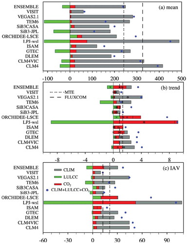
Figure 1. Contributions to the (a) annual mean (mean) (units: g C m⁻² yr⁻¹), (b) trend (units: Tg C yr⁻²) (1 Tg C = 10¹² g C), and (c) interannual variability (IAV) (units: Tg C yr⁻¹) of GPP on the Tibetan Plateau from climate (CLIM), land-use and land-cover change (LULCC), and rising CO₂ by MsTMIP models. The gray bars, red bars, green bars, and blue dots indicate trends driven by CLIM, CO₂, LULCC, and all of them (SG3), respectively. An asterisk in (b) indicates that the trend is statistically significant at the 0.01 (p < 0.01) level.

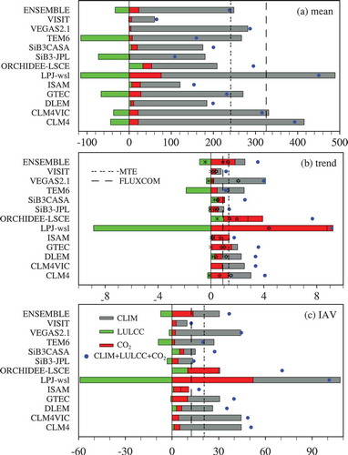
Figure 1(a) shows the contributions to the annual mean GPP from LULCC, rising CO₂, and climate change. The mean annual GPP of the TP is mainly driven by climate change, while LULCC and a rising atmospheric CO₂ concentration have a small effect. The annual mean GPP from ENSEMBLE is 238 g C m⁻² yr⁻¹, which is similar to that determined with the MTE data (241 g C m⁻² yr⁻¹) and lower than with FLUXCOM (325 g C m⁻² yr⁻¹). Most models show a negative contribution to the annual mean TP GPP values in terms of LULCC, where the highest negative contribution is in TEM6 (−71.93%, Table 1). Otherwise, DLEM, ISAM, ORCHIDEE-LSCE, SiB3CASA, and VEGAS2.1 show a positive contribution, where ORCHIDEE-LSCE shows the highest positive contribution (11.03%). However, the contributions to the annual mean GPP values from CO₂ are positive, where ORCHIDEE-LSCE is more sensitive to CO₂ (18.19%). As for ENSEMBLE, −14% is from LULCC, and 10% is from CO₂. In contrast, considerable uncertainties remain about the contributions to the annual mean TP GPP values from LULCC.

3.2 Trends

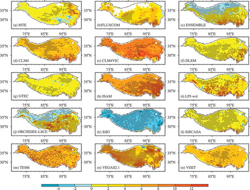
The spatial patterns of the linear trends of GPP exhibit significant increases in the MTE data and FLUXCOM (Figure 2). Most models show significant increasing trends, except for SiB3. Obviously, ENSEMBLE captures the GPP trends over the southern TP better than most of the single models. However, the multi-model ensemble mean values of MsTMIP (SG3) show a negative trend over the northern TP.

Figure 2. Spatial patterns of the linear trends of GPP from the MTE, FLUXCOM, and MsTMIP models (from the SG3 simulation) over the Tibetan Plateau from 1982 to 2010. ENSEMBLE is the ensemble mean of the 12 MsTMIP models. The black dots indicate that the trends are statistically significant (p < 0.01).

Climate change results in a significantly increased annual GPP (2.6 Tg C yr⁻²) during the past 29 years (Figure 3), which contributes about 72.61% (± 50.90%) to the GPP trends from ENSEMBLE (Table 1). LULCC and rising atmospheric CO₂ concentration have a very large influence on the annual GPP trends (−24.24% and 51.63%) compared with the annual mean values and IAVs. In contrast with the FLUXCOM data (0.9 Tg C yr⁻²), all of the models overestimate the trends on the TP, while with the MTE data (1.3 Tg C yr⁻²) most models overestimate the trends, except for VISIT (1.1 Tg C yr⁻²) (Figure 1(b)). Due to the CO₂ fertilization effect, rising CO₂ contributes to the significant positive trends in the annual GPP of the TP. As for LULCC, four TBMs (CLM4, LPJ-wsl, TEP6, and VEGAS2.1) show negative trends, three (DLEM, ORCHIDEE-LSCE, and SiB3CASA) show positive trends, and five (CLM4VIC, GTEC, ISAM, SiB3-JPL, and VISIT) show negligible trends, where ENSEMBLE shows the largest significant negative trend, while the largest increase, 1.0 Tg C yr⁻², is found by ORCHIDEE-LSCE. In other words, the uncertainties associated with the contribution from LULCC are still considerable. During 1981–2010, the MTE and FLUXCOM estimates suggest that the trends of the TP’s GPP are 1.3 Tg C yr⁻² and 0.9 Tg C yr⁻², respectively. However, the multi-model ensemble mean values of MsTMIP for the three sensitivity model simulations (SG1: 2.6 Tg C yr⁻²; SG2: 1.7 Tg C yr⁻²; SG3: 3.5 Tg C yr⁻²) all show overestimates.

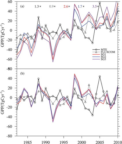
Figure 3. Interannual changes of TP GPP from the MTE (black line with circular markers), FLUXCOM (gray line with triangle markers), and the ensemble mean of the 12 MsTMIP models: SG1 (red), SG2 (blue), SG3 (purple). Panel (b) uses the detrended annual time-series data. The anomalies were calculated as the difference between annual GPP and the long-term mean over the period for each data source. The numbers located at the top of each figure indicate the linear trends of SG1 (red), SG2 (blue), SG3 (purple), MTE (black), and FLUXCOM (gray) with units of Tg C yr⁻². An asterisk indicates that the trend is statistically significant (p < 0.01).

3.3 IAVs

Figure 3 shows the interannual changes of GPP over the TP, where the annual mean GPP values from the MTE and FLUXCOM data exhibit significant increasing trends (MTE is 1.5 Pg C yr⁻² and FLUXCOM is 0.9 Pg C yr⁻²) (p < 0.05) during 1982–2010. However, the three MsTMIP simulations all show a slight overestimation. Compared to SG1 (red line) with the prescribed land cover, LULCC (blue line) results in decreased GPP trends over the TP, which are mainly related to land conversion including native grassland to monoculture (Zhao et al. 2015; Figure 3). On the contrary, elevated CO₂ concentration significantly increases plant growth and thus leads to more strongly increasing GPP trends (SG3, purple line).

Climate remains the main driver for the IAVs of GPP over the TP, except for ISAM (Table 1). During 1981–2010, the MTE data suggest that the IAV of GPP over the TP is 21 Tg C yr⁻¹, while FLUXCOM suggests a rate of 12 Tg C yr⁻¹. Meanwhile, the multi-model ensemble mean values of MsTMIP for SG3 show an overestimation (Figure 1(c)). In contrast, the contributions of LULCC and rising CO₂ to the IAVs of the TP’s GPP are relatively lower (−20% and 37%), higher than contributions to annual mean GPP (Table 1), where LULCC decreases the IAV by ~7 Tg C yr⁻¹, whereas rising CO₂ leads to an increase (~14 Tg C yr⁻¹) (Figure 1(c) and Table 1).

When analyzing these results, it is worth noting the significant uncertainties with large standard deviations among ENSEMBLE’s contributions from LULCC, rising CO₂, and climate change. For CO₂, the GPP determined by ISAM explains the largest fraction (61.71%) of the IAV, followed by LPJ-wsl (51.62%) and ORCHIDEE-LSCE (42.44%). In addition, for LULCC, LPJ-wsl shows the largest negative contribution (−58.56%), while SiB3CASA shows the largest positive contribution (17.62%).

4. Conclusions

In this study, a multi-model analysis that considered 12 MsTMIP-based models was used to investigate the contributions of climate change and anthropogenic activities (LULCC and rising CO₂ concentration) to the IAVs and trends of GPP over the TP. The ensemble simulation results of MsTMIP were also compared with independent upscaled GPP products from MTE (Jung et al. 2011) and FLUXCOM (Tramontana et al. 2016; Jung et al. 2017).

Compared to the single models, the simulated GPP from the multi-model ensemble, driven by common climate forcing, LULCC, and CO₂, showed higher spatial correlations (> 0.80) with the MTE and FLUXCOM data over the TP. In general, climate change was the dominant controlling factor for the trends, IAVs, and the annual mean of the TP’s GPP. The overall rise in CO₂ (mainly fertilization effect) would have enhanced plant photosynthesis, and hence increased the GPP of the TP, resulting in an increased annual mean (~23 g C m⁻² yr⁻¹) and IAV (~14 Tg C yr⁻¹). Compared with the annual mean GPP (respectively, −14.08% ± 26.36% and 9.66% ± 5.72%), LULCC and rising atmospheric CO₂ concentration had a larger influence on the IAVs (−19.81% ± 22.27% and 36.94% ± 17.33%) and trends (−24.24% ± 53.28% and 51.63% ± 24.49%). However, LULCC had considerable associated uncertainties, and four TBMs showed that LULCC decreased the GPP of the TP, three showed it increased the GPP, and five showed negligible trends. Therefore, the impacts of land-use change are important on the TP. In addition, the experimental design with respect to the set of prescribed LULCCs in SG1 and the fixed CO₂ concentration in SG1 and SG2 may have had some effects on the analysis results in this study. For example, SG2, with a CO₂ concentration of the first year (1801) versus the last year (2010) may have led to roughly opposite results between SG2 and SG3, while a CO₂ concentration of the middle year may have resulted in a more moderate difference.

Acknowledgments

The finalized MsTMIP data products are archived at http://daac.ornl.gov. The MTE data and flux tower–based GPP observations were downloaded freely from the Max Planck Institute for Biogeochemistry (https://www.bgc-jena.mpg.de/). The FLUXCOM data that supported the findings of this study are available from the Data Portal of the Max Planck Institute for Biogeochemistry (https://www.bgc-jena.mpg.de/geodb/projects/Home.php) with the identifier doi:10.17871/FLUXCOM_RS_METEO_CRUNCEPv6_1980_2013_v1.

Disclosure statement

No potential conflict of interest was reported by the authors.

Supplemental material

Supplemental data for this article can be accessed here.

Additional information

Funding

This research was supported by the National Key R & D Program of China [grant number 2018YFC1506602], the Key Research Program of Frontier Sciences, Chinese Academy of Sciences [grant number QYZDY-SSW-DQC012], and the National Natural Science Foundation of China [grant numbers 41830967 and 41575096].

References

- Anav, A., P. Friedlingstein, C. Beer, P. Ciais, A. Harper, C. Jones, G. Murray-Tortarolo, et al. 2015. “Spatiotemporal Patterns of Terrestrial Gross Primary Production: A Review.” Reviews of Geophysics 53: 785–818. doi:10.1002/2015RG000483.
- Babel, W., T. Biermann, H. Coners, E. Falge, E. Seeber, J. Ingrisch, P. M. Schleuß, et al. 2014. “Pasture Degradation Modifies the Water and Carbon Cycles of the Tibetan Highlands.” Biogeosciences 11 (23): 6633–6656.
- Ciais, P., G. Bala, L. Bopp, V. Brovkin, J. Canadell, A. Chhabra, R. DeFries, et al. 2013. “Carbon and Other Biogeochemical Cycles.” In Climate Change 2013: The Physical Science Basis. Contribution of Working Group I to the Fifth Assessment Report of the Intergovernmental Panel on Climate Change, edited by Stocker, T. F, Qin, D, Plattner, G. K, Tignor, M, Allen, S. K, Boschung, J, Nauels, A, Xia, Y, Bex, V, and Midgley, P. M, 465–570. Cambridge, UK and New York, NY, USA: Cambridge University Press.
- Friedlingstein, P., R. A. Houghton, G. Marland, J. Hackler, T. A. Boden, T. J. Conway, T. J. Canadell, et al. 2010. “Update on CO2 Emissions.” Nature Geoscience 3 (12): 811–812. doi:10.1038/ngeo1022.
- Hagedorn, R., F. J. Doblas-Reyes, and T. N. Palmer. 2005. “The Rationale behind the Success of Multi-model Ensembles in Seasonal Forecasting – I Basic Concept.” Tellus A: Dynamic Meteorology and Oceanography 57 (3): 219–233.
- Huntzinger, D. N., C. Schwalm, A. M. Michalak, K. Schaefer, A. W. King, Y. Wei, A. Jacobson, et al. 2013. “The North American Carbon Program Multi-scale Synthesis and Terrestrial Model Intercomparison Project: Part 1: Overview and Experimental Design.” Geoscientific Model Development 6 (6): 2121–2133. doi:10.5194/gmd-6-2121-2013.
- IPCC. 2013. Climate Change 2013 – The Physical Science Basis. Working Group I Contribution to the Fifth Assessment Report of the Intergovernmental Panel on Climate Change. Cambridge: Cambridge University Press. doi:10.1017/CBO9781107415324.
- Ito, A., K. Nishina, C. P. O. Reyer, L. François, A. J. Henrot, G. Munhoven, I. Jacquemin, et al. 2017. “Photosynthetic Productivity and Its Efficiencies in ISIMIP2a Biome Models: Benchmarking for Impact Assessment Studies.” Environmental Research Letters 12 (8): 085001. doi:10.1088/1748-9326/aa7a19.
- Jung, M., M. Reichstein, and A. Bondeau. 2009. “Towards Global Empirical Upscaling of FLUXNET Eddy Covariance Observations: Validation of a Model Tree Ensemble Approach Using a Biosphere Model.” Biogeosciences 6: 2001–2013. doi:10.5194/bg–6–2001-2009.
- Jung, M., M. Reichstein, H. Margolis, A. Cescatti, A. Richardson, M. Arain, A. Arneth, et al. 2011. “Global Patterns of Land-atmosphere Fluxes of Carbon Dioxide, Latent Heat, and Sensible Heat Derived from Eddy Covariance, Satellite, and Meteorological Observations.” Journal of Geophysical Reseach 116: G00J07. doi:10.1029/2010JG001566.
- Jung, M., M. Reichstein, C. R. Schwalm, C. Huntingford, S. Sitch, A. Ahlström, A. Arneth, et al. 2017. “Compensatory Water Effects Link Yearly Global Land CO2 Sink Changes to Temperature.” Nature 541 (7638): 516–520. doi:10.1038/nature20780.
- Liu, J. G., B. H. Jia, Z. H. Xie, and C. X. Shi. 2016a. “Ensemble Simulation of Land Evapotranspiration in China Based on a Multi-forcing and Multi-model Approach.” Advances in Atmospheric Sciences 33 (6): 673–684. doi:10.1007/s00376-016-5213-0.
- Liu, L., X. Zhang, A. Donnelly, and X. Liu. 2016b. “Interannual Variations in Spring Phenology and Their Response to Climate Change across the Tibetan Plateau from 1982 to 2013.” International Journal of Biometeorology 60 (10): 1–13. doi:10.1007/s00484-016-1147-6.
- Ma, M. N., and W. P. Yuan. 2017. “Model Differences in Estimation of Gross Primary Productivity of the Qinghai-Tibet Plateau.” Remote Sensing Technology and Application 32 (3): 406–418. (in Chinese).
- Piao, S. L., G. D. Yin, J. G. Tan, L. Cheng, M. T. Huang, Y. Li, J. F. Mao, et al. 2015. “Detection and Attribution of Vegetation Greening Trend in China over the Last 30 Years.” Global Change Biology 21: 1601–1609. doi:10.1111/gcb.12795.
- Qiu, L., and X. Liu. 2016. “Sensitivity Analysis of Modelled Responses of Vegetation Dynamics on the Tibetan Plateau to Doubled CO2 and Associated Climate Change.” Theoretical and Applied Climatology 124 (1–2): 229–239. doi:10.1007/s00704-015-1414-1.
- Schwalm, C. R., D. N. Huntzinger, J. B. Fisher, A. M. Michalak, K. Bowen, P. Ciais, and R. Cook. 2015. “Toward “Optimal” Integration of Terrestrial Biosphere Models.” Geophysical Research Letters 42 (11): 4418–4428. doi:10.1002/2015GL064002.
- Sen, P. K. 1968. “Estimates of the Regression Coefficient Based on Kendall’s Tau.” Publications of the American Statistical Association 63 (324): 1379–1389. doi:10.1080/01621459.1968.10480934.
- Shang, Z. H., M. J. Gibb, F. Leiber, M. Ismail, L. M. Ding, X. S. Guo, and R. J. Long. 2014. “The Sustainable Development of Grassland-livestock Systems on the Tibetan Plateau: Problems, Strategies and Prospects.” The Rangeland Journal 36 (3): 267–296. doi:10.1071/Rj14008.
- Tramontana, G., M. Jung, C. R. Schwalm, K. Ichii, G. Camps-Valls, B. Ráduly, M. Reichstein, et al. 2016. “Predicting Carbon Dioxide and Energy Fluxes across Global Fluxnet Sites with Regression Algorithms.” Biogeosciences 13 (14): 4291–4313. doi:10.5194/bg-13-4291-2016.
- Valentini, R., A. Arneth, A. Bombelli, S. Castaldi, R. Cazzolla Gatti, F. Chevallier, P. Ciais, et al. 2014. “A Full Greenhouse Gases Budget of Africa: Synthesis, Uncertainties, and Vulnerabilities.” Biogeosciences 11: 381–407. doi:10.5194/bg-11-381-2014.
- Wei, Y., S. Liu, D. N. Huntzinger, A. M. Michalak, N. Viovy, W. M. Post, C. R. Schwalm, et al. 2014. “The North American Carbon Program Multi-scale Synthesis and Terrestrial Model Intercomparison Project–Part 2: Environmental Driver Data”. Geoscientific Model Development 7: 2875–2893. doi:10.5194/gmd-7-2875-2014.
- Zhang, Y., Q. Z. Gao, S. K. Dong, S. K. Liu, X. X. Wang, X. K. Su, Y. Y. Li, et al. 2015. “Effects of Grazing and Climate Warming on Plant Diversity, Productivity and Living State in the Alpine Rangelands and Cultivated Grasslands of the Qinghai-Tibetan Plateau.” The Rangeland Journal 37 (1): 57–65. doi:10.1071/RJ14080.
- Zhang, Y. L., W. Qi, C. P. Zhou, M. J. Ding, L. S. Liu, J. G. Gao, W. Q. Bai, et al. 2014. “Spatial and Temporal Variability in the Net Primary Production of Alpine Grassland on the Tibetan Plateau since 1982.” Journal of Geographical Sciences 24 (2): 269–287. doi:10.1007/s11442-014-1087-1.
- Zhao, L., D. D. Chen, N. Zhao, Q. Li, Q. Cheng, C. Y. Luo, S. X. Xu, et al. 2015. “Responses of Carbon Transfer, Partitioning, and Residence Time to Land Use in the Plant-soil System of an Alpine Meadow on the Qinghai-Tibetan Plateau.” Biology and Fertility of Soils 51 (7): 781–790. doi:10.1007/s00374-015-1024-1.